Credit scoring by segmented modelling

(1)

University of Tartu

Faculty of Science and Technology

Institute of Mathematics and Statistics

Tevfik Can Özay

Credit Scoring by Segmented Modelling

Financial Mathematics

Master Thesis (15 ECTS)

Supervisor: Kalev Pärna

(2)

Credit Scoring by Segmented Modelling

Master’s thesis Tevfik Can Özay

Abstract. This study is devoted to small loan evaluation modelling which is known as credit scoring. Credit scoring models help the decision takers (such as credit offices, banks …) decide customers’ creditworthiness in short time without prejudice. Main goal of this master thesis was to understand feasibility and effectiveness of credit scoring model by using logistic regression technique and obtaining important variables for credits scoring models. Furthermore we targeted to reveal how segmentation (creating different score cards for different age groups) can help to predict more accurately. In this study, we worked with real data which was provided by local company in Estonia. In conclusion, our results showed that credit scoring by logistic regression helped to discriminate good customers effectively and the use of segmentation improves the model’s accuracy.

CERCS research specialisation: P160 Statistics, operations research, programming, actuarial mathematics.

Key words: Credit Scoring, Logistic Regression, Regression Analysis

Krediidiskooring segmenteeritud mudelite abil

Magistritöö Tevfik Can Özay

Lühikokkuvõte. Antud töö on pühendatud väikelaenude hindamise modelleerimisele, mis on tuntud krediidiskooringu nime all. Krediidiskooring võimaldab laenuandjatel (laenuasutused, pangad) otsustada erapooletult laenutaotleja krediidikõlblikkuse üle. Antud töö peaeesmärgiks oli välja selgitada logistilise regressiooni kasutamisvõimalused krediidiskooringu mudeli loomisel ning tuvastada sellise mudeli tähtsad argumenttunnused. Lisaks on püütud välja selgitada segmenteerimise osa mudeli prognoosivõime parandamisel, luues erinevatele vanuserühmadele erinevad mudelid. Töö empiirilises osas on kasutatud reaalseid andmeid. Kokkuvõttes näitavad töö tulemused, et logistiline regression võimaldab efektiivselt eristada häid kliente halbadest ning et segmenteerimine aitab parandada mudeli täpsust.

CERCS teaduseriala: P160 Statistika, operatsioonianalüüs, programmeerimine, finants- ja kindlustusmatemaatika.

(3)

2

Introduction

Nowadays credit sector is continuing to grow rapidly and in the meantime importance of credit scoring and managing the process of credit assessments is getting more critical for lenders, credit offices and banks. Emerging issue is to handle dramatically increasing number of applications whether candidates are eligible to take credit or not and having limited time to evaluate all these applications. Most of the professional lenders are already using statistical modelling techniques to assess their potential candidates. On the other hand, traditional judgmental assessment is still in common usage even though it is quite long process and it is needed massive experience and trainings. Therefore credit scoring has very important role which provides opportunity to assess candidates in short period and without prejudice. In this point, there are so many doubts about which statistical methods are more helpful and feasible for different credits such as small loans, mortgage … And there are many questions about what is benefit of creating different scorecards/models for different groups? Is creating different scorecards worth to work on it? How effectively does it help to improve accuracy of predictions? Increased competition and growing pressures for revenue generation have led credit-granting and other financial institutions to search for more effective ways to attract new creditworthy customers and at the same time, control losses [6]. Therefore professionals are always trying to find better and more accurate method for credits scoring in order to have better predictions. In this study, we will work with logistic regression which is one of the most popular methods for creating credit scoring model recently and analysis is performed by IBM SPSS 21.

Main purpose of this master thesis is 1) to show effectiveness of credit scoring model by logistic regression method; 2) to detect significant parameters for credit scoring model which may help further researches; 3) to understand importance of segmentation by comparing segmented models with one single model for everyone. With this purposes, we consider classification table as main indicator in this study which is one of the ways to see the percentage of correct prediction of each model.

The first chapter focuses on what is credit scoring and gives an historical background. It is followed by logistic regression in Chapter 2. The next chapter deals with framework of empirical study and data preparation. We emphasize our target population, dependent and independent variables, detecting outliers and how we treat missing values in this study. In Chapter 4, we concentrate on creating one single model for all clients by using logistic regression and in Chapter 5, we create 4 different models for the same number of age groups.

(5)

4 In chapter 6, there is summary of our results and comparison of two different approaches in order to see benefits from creating different score cards for different age groups.

(6)

5

1 Credit Scoring

1.1. What is Credit Scoring?

In current context, ‘credit’ simply means, “buy now, pay later”, whether the purchase is for short-term consumption, durable goods and other assets that provide users with valuable services or productive enterprises. The word ‘credit’ comes from the old Latin word ‘credo’, which means, ‘trust in’ or ‘rely on’. If you lend something to somebody, then you have to have trust in him or her to honor the obligation. [1]

Credit Scoring is set of decisions model and their underlying techniques that aid lenders in the granting of consumer credit. These techniques decide who will get credit, how much credit they should get, and what operational strategies will enhance the profitability of borrowers to the lenders. [8] According to Anderson, Credit scoring is the use of statistical models to transform relevant data into numerical measures that guide credit decisions.

1.2 History of Credit Scoring

Following overview is based on [8]

Mostly it is believed that people started borrowing and repaying while human started to communicate with each other. The first recorded instance of credit comes from ancient Babylon. According to stone table around 2000 BC, two shekels of silver have been borrowed by Mas-Schamach, son of Adadrimeni, from the sun priestess Amat-Schamach, the daughter of Warad-Enlil. He will pay the Sun-God’s interest. At the time of harvest he will pay back the sum and interest upon it.

The next thousands years, the “Dark Ages” of European history, saw a little development in credit, but by the time of the Crusades in the thirteen century, pawn shop has been developed however Crusades had no interest in this time. At the same time, merchants quickly saw the possibilities and by 1350 commercial pawn shops charging interest were found throughout Europe. During the middle ages, there was ongoing debate on the morality of charging interest on loans. The outcome of the debate in Europe was that if the lender levied small charges, this was interest and was acceptable, but large charges were usury, which was bad. Even Shakespeare got into this debate with his portrait of the Merchant of Venice. Also at this time, kings and potentates began to have to borrow in order to finance their wars and other expenses.

(7)

6 Lending was more politics than business. The rise of the middle classes in the 1800’s led to the formation of a number of private banks, which were willing to give bank overdrafts to fund businesses and living expenses. However, this start of consumer credit was restricted to a very small proportion of the population.

The real revolution started in the 1920’s when consumers started to buy motor cars. Finance companies were developed to respond to this need and experienced rapid growth before World War II. At the same time, mail-order companies began to grow as consumers in smaller towns demanded the clothes and household items that were available only in larger population centers. These were advertised in catalogues, and the companies were willing to send the goods on credit and allow customers to pay over an extended period.

While the history of credit stretches back 5000 years, the history of credit scoring is only 50 years old. Credit scoring is essentially a way to identify different groups in a population when one cannot see the characteristic that defines the groups.

During the 1930’s some mail-order companies had introduced numerical scoring systems to try to overcome the inconsistencies in credit decisions across credit analysts. With the start of the World War II, all the finance houses and mail-order firms began to experience difficulties with credit management. Hence the firms had the analysts write down the rules of thumb they used to decide to whom to give loans. These rules were then used by non-experts to help make credit decisions.

It did not take long after the war ended for some folks to connect the automation of credit decisions and the classification techniques being developed in statistics and to see the benefit of using statistically derived models in lending decisions. The first consultancy was formed in San Francisco by Bill Fair and Earl Isaac in the early 1950’s, and their clients were mainly fiancé houses, retailers and mail-order firms. The arrival of credit cards in the late 1960’s made the banks and other credit card issuers realize the usefulness of credit scoring. The number of people applying for credit cards each day made it impossible in both economics and manpower terms to do anything but automate the lending decision. The growth in computing power made this possible. The organizations found credit scoring to be a much better predictor than any judgmental scheme and default rates dropped by 50 percent or more. In the 1980’s, the success of credit scoring in credit cards meant that banks started using scoring for other products, like personal loans, while in the last few years, scoring has been used for home loans and small business loans. In the 1990’s, growth in direct marketing led to the use of scorecards to improve

(8)

7 the response rate to advertising campaigns. Advances in computing allowed other techniques to be tried to build scorecards. In the 1980’s, logistic regression and linear programming, the two main stalwarts of today’s card builder, were introduced.

1.3 Credit Assessment Before Credit Scoring and Why Credit Scoring

This section is based on [8] and [5]

In early 1960’s, lenders had some difficulties to assess their customers individual applications. Traditional assessment needed so long time for evaluating only one candidate. Traditional assessment simply relied on evaluating borrowers’ characteristic, ability to pay back his or her debt and individual experience of investigator. Generally manager took responsibility to assess their clients. Investigator evaluated the length of relationship with customer, likelihood of payment, assess stability, honesty and other characteristics. If manager did not convince and had doubts about customers, it meant further investigations and spent more time for single candidate. Process was obviously slow and inconsistent. There were plenty of disadvantages for processing traditional assessment;

 Task manager needed education and so long training period,

 Process was extremely slow and it was big obstacle to prevent having more customers/lenders,

 There was no unbiased assessment opportunities,

 Borrower needed to have quite long history to be invited investigation appointment. Rapidly growing credit sector needed new assessment system. And many changes occurred in lender and borrower environment. Some of these changes were as follows;

 Banks changed their market position considerably and began to market their products. This in turn meant that they had to sell products to customers not only whom they hardly knew but whom they had enticed.

 There was phenomenal growth in credit cards. Sales authorizations of this products meant that there had to be a mechanism for making a lending decision very quickly and around the clock. Also, volumes of applications were such that the manager or other trained credit analyst could would not have the time or opportunity to interview all the applicants. Clearly there would be insufficient numbers of experienced bank managers to handle the volume. During the 1980’s, a handful of U.K. operations were dealing with several thousand applications each day.

(9)

8  Banking practice changed emphasis. Previously, banks had focused almost exclusively on large lending and corporate customers. Now consumer lending was an important and growing part of the bank. It would still be a minority part by value but was becoming significant. Bank could not control the quality across a branch network of hundreds or thousands of braches and mistakes were made. With corporate lending, the aim was usually to avoid any losses. However, banks began to realize that with consumer lending, the aim should not be to avoid any losses but to maximize profits. Keeping losses under control is part of that, but one could maximize profits by taking on a small controlled level of bad debts and so expand the consumer lending book.

1.4 Statistical Methods For Building Credits Scoring

When credit scoring was first developed in the 1950s and 1960s, the only methods used were statistical discrimination and classification methods. Even today statistical methods are by far the most common methods for building credit scorecards. Statistical techniques allow one to identify and remove unimportant characteristics and ensure that all the important characteristics remain in model.

Although statistical methods were the first to be used to build scoring system and they remained the most important methods, there have been changes in the methods used during the intervening 40 years. Initially, the methods were based around the discrimination methods suggested by Fisher (1936) for general classification problems. This led to a linear scorecard based on the Fisher linear discriminant function. The assumptions that were needed to ensure that this was the best way to discriminate between good and bad potential customers were extremely restrictive and clearly did not hold in practice, although the scorecards produced were very robust. The Fisher approach could be viewed as a form of linear regression, and this led to an investigation of other forms of regression. By far the most successful of these is Logistic Regression, which has taken over from the linear regression-discriminant analysis approach as the most common statistical method. Another approach that has found favor over the last 20 years is the classification tree approach. With this, one splits the set of applicants into a number of different subgroups depending on their attributes and then classifies each subgroup as satisfactory or unsatisfactory. Although this does not give a weight to each of the attributes as the linear scorecards does. There are also few non parametric approach based on nearest neighbors. [8]

(10)

9

2 Logistic Regression

This section is based on [9] and [6]

In the classical regression framework, we are interested in modeling a continuous response variable 𝑦 as a function of one or more predictor variables. Most regression problems are of this type. However, there are numerous examples where the response of interest is not continuous, but binary. Consider an experiment where the measured outcome of interest is either a success or failure, which we can code as a 1 or a 0. The probability of a success or failure may depend on a set of predictor variables. One idea on how to model such data is to simply fit a regression with the goal of estimating the probability of success given some values of the predictor. However, this approach will not work because probabilities are constrained to fall between 0 and 1. In the classic regression setup with a continuous response, the predicted values can range over all real numbers. Therefore, a different modelling technique is needed. That is, in with a binary outcome, regression of 𝑦 on 𝑥 is a conditional probability. If we label

𝑦 = 1 as a “success”, then the goal is to model the probability of success given 𝑥. The approach

to this problem illustrated here is known as Logistic Regression.

Logistic regression, like most other predictive modeling methods, uses a set of predictor characteristics to predict the likelihood (or probability) of a specific outcome (the target). The equation for the logit transformation of a probability of an event is shown by:

𝑙𝑜𝑔𝑖𝑡(𝜋) = 𝑙𝑛 ( 𝜋

1 − 𝜋) = 𝛽0+ 𝛽1𝑥1+ 𝛽2𝑥2+ ⋯ + 𝛽𝑘𝑥𝑘

π = posterior probability of “event”, given inputs, x = input variables,

𝛽₀ = intercept of regression line,

𝛽_𝑖 = parameters

Logistic Regression function for probability of individual is good:

π = ( 𝑒

𝛽0+𝛽1𝑋1+𝛽2𝑋2+⋯+𝛽𝑘𝑋𝑘

1 + 𝑒𝛽0+𝛽1𝑋1+𝛽2𝑋2+⋯+𝛽𝑘𝑋𝑘)

(11)

10

(1 − π) = (1 − 𝑒

𝛽0+𝛽1𝑋1+𝛽2𝑋2+⋯+𝛽𝑘𝑋𝑘

1 + 𝑒𝛽0+𝛽1𝑋1+𝛽2𝑋2+⋯+𝛽𝑘𝑋𝑘)

Regression can be run to find out the best possible model using all options available. This is commonly known as “all possible” regression techniques and is computationally intensive, especially if there are a lot of independent input characteristics. Far more commonly used are the three types of stepwise logistic regression techniques:

Forward Selection: First selects the best one characteristic model based on the individual predictive power of each characteristic, then adds further characteristics to this model to create the best two, three, four, and so on characteristic models incrementally, until no remaining characteristics have p-values of less than some significant level , or univariate Chi Square above a determined level. This method is efficient, but can be weak if there are too many characteristics or high correlation.

Backward Elimination: The opposite of forward selection, this method starts with all the characteristics in the model and sequentially eliminates characteristics that are considered the least significant, given the other characteristics in the model, until all the remaining characteristics have a p-value below a significant level or based on some other measure of multivariate significance. This method allows variables of lower significance a higher chance to enter the model, much more than forward or stepwise, whereby one or two powerful variables can dominate.

Stepwise: A combination of the above two techniques, this involves adding and removing characteristics dynamically from the scorecard in each step until the best combination is reached. A user can set minimum p-values required to be added to the model, or to be kept in the model.

2.1 Why Logistic Regression Analysis for Credit Scoring

The Linear regression model provides a powerful device for organizing data analysis. Researchers focus on the explanation of dependent variable, 𝑌, as a function of multiple independent variables, from 𝑋₁ to 𝑋_𝑘 . Models are specified, variables are measured and equations are estimated with ordinary least squares. All goes well if the classical linear regression assumptions are met. However several assumptions are likely to be unmet if the

(12)

11 dependent variable has only two or three response categories. In particular, with a dichotomous dependent variable, assumptions of homoscedasticity, linearity and normality are violated and OLS estimates are inefficient at best. The maximum likelihood estimation of a logistic regression overcomes inefficiency, transforming 𝑌 (1,0) into a logit. [4]

As we have already noted, logistic regression is one of the most frequently used statistical model used in credit scoring. It is the best to show probability of default and risk of decision. [3] When we consider Credit Scoring models, our main purpose is understanding difference between being Good Customer and Bad Customer. Status of customer have two options in this case. It means binary dependent variable where Logistic Regression provides best approach to deal with categorical dependent variable.

(13)

12

3 Framework of Study and Data Preparation

3.1 Target population

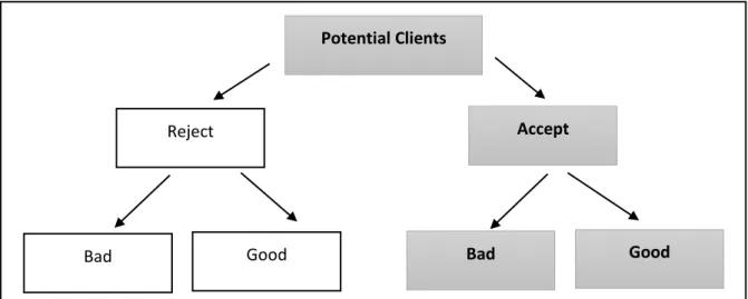
There are two most common approaches to create the credit scoring model. One is based on all component of population; Accepted bad and good clients and rejected bad and good clients. Other approach is creating the credit scoring model by based only on accepted clients who were eligible to get loan by decision technique of lender, however this method does not include rejected potential clients. In our study, our data allows us to use only second approach. There is no information about rejected people in data and therefore we will consider only accepted clients in our model. Our training data in this study is provided by one local company in Estonia.

Figure 1: Components of Credit Scoring Model Population

Good/Bad Clients: Basically good clients are people who paid back their debts as scheduled and bad clients who did not pay back their debt as scheduled. Needless to say, bankruptcy and fraud is considered as bad clients.

Delinquency; occurs when a borrower fails to make a scheduled payment on a loan. Since loan payments are typically due monthly, lending industry customarily categorizes delinquent loans as either 30, 60, 90 or 120 or more days late depending on the length of time oldest unpaid loan payment has been overdue. [2]

Actual good client who paid their debts as scheduled however also some credit scoring systems may accept some problematic payment process as good client too. There are some situation where credit offices are able to consider them as good client even though they had problems to pay their debt as they scheduled:

Potential Clients

Accept

Bad Good

Reject

(14)

13

- Borrower chooses to give the lender title of the property

- Lender agrees to renegotiate or modify the term of loan and forgives some or all of the delinquent principal and interest payments. (Loan modifications may take many form including change in the interest rate on the loan and extension of the length of the loan.) [2]

3.2 Variables

Variables Explanation

Status * Good clients(Y=1) who paid back their debts without facing any problem and bad clients(Y=0)

Sex Female/Male

Age Age of customers

Region Countries such

Language Mother tongue

Sum Amount money is taken from bank (loan sum)

Period Loan period in days

Income Monthly income in EUR

Outcome Monthly outcome in EUR

Family Marriage Status

Education Education level

WorkExperience Clients who has more than one year experience and less than one year

Children Number of Children

Estate Number of real estate units

AlertsTotal Total number of payment problems

AlertsActive Number of active payment problems

AlertsClosed Number of closed payment problems

*Dependent Variable

Table 1. Dependent and Independent Variables

Alerts Closed is highly correlated with Alerts Active (0.96) and therefore we did not include it in our model.

3.3 Classification of Regions

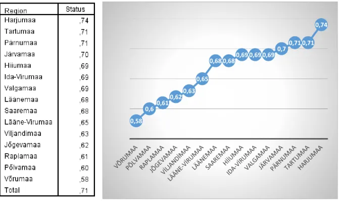
Estonia is divided into fifteen countries/regions. Capital city of Estonia is Tallinn and it is located in Harjumaa region. Second biggest city is Tartu and Tartu is located in Tartumaa region. Other countries are Pärnumaa, Järvamaa, Hiiuma, Ida-Virumaa, Valgamaa, Läänemaa, Saaremaa, Lääne-Virymaa, Viljandimaa, Jõgevamaa, Raplamaa, Põlvamaa and Võrumaa.

(15)

14 Figure 2. Means of Regions

Regions are reorganized by dendrogram of hierarchical clustering method of SPSS which helps to merge similar clusters. Clustering starts with every region in individual cluster and ends up with every region in one cluster regarding mean. We used same approach for age subgroups. This approach helps us to determine which regions should be merged at each step.

Figure 3. Countries Dendrogram 0,58 0,6 0,61 0,620,63 0,65 0,68 0,680,69 0,69 0,69 0,70,71 0,71 0,74

(16)

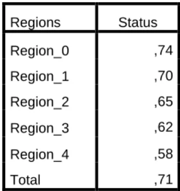
15 When distance indicator is 4, we have 5 regions groups by using clustering method. First region group is consisted of Harjumaa country. Region_1 group is consist of Tartumaa, Hiiuma, Ida-Virumaa, Valgamaa, Saarema, Läänem, Pärnumaa and Järvamaa countries. Region_2 group is consist of Lääne-Virumaa. Region_3 group is consisted of Põlvamaa, Raplamaa, Viljandimaa and Jõgevamaa countries and last region group is consisted of only Võrumaa. Probability of being good customer in these groups is 0.75, 0.70, 0.65, 0.62 and 0.58, respectively.

Regions Status Region_0 ,74 Region_1 ,70 Region_2 ,65 Region_3 ,62 Region_4 ,58 Total ,71

Table 2. Means of Regions After Classification

3.4 Missing Values and Detection of Outliers

In Statistics, missing data, or missing values, occur when no data value is stored for the variable in an observation. Missing data are a common occurrence and can have a significant effect on the conclusions that can be drawn from the data. [13]

There is four main ways to deal with missing values;

1. Exclude all data with missing values.

2. Exclude characteristics or records that have significant ( more than 50%) missing values from the model, especially if the level of missing is expected to continue in the future. 3. The “missing values” can be treated as a separate attribute.

4. Impute missing values using statistical techniques. [6]

In statistics, an outlier is an observation point that is distant from other observations. [11] Outliers are values that fall outside of the normal range of value for a certain characteristic. These numbers may negatively affect the regression result, and are usually excluded. [6]

In our study, logistic regression requires complete data without missing cases and therefore we preferred first approach and we assumed that missing data is excluded. Also we preferred to use Box-plot method for detecting outliers. Box-plot method provides visual representation of

(17)

16 dispersion of the data. This graphic has the lower quartile, 𝑄₁, and upper quartile , 𝑄₃ , with median (50th percentile). Upper and lower bounds are set a fixed distance with range between

𝑄3− 𝑄1 .Upper and Lower fences to set at 1.5 times the interquartile range. Observations where are located out of these fences are potentially outliers/extreme values. One of the most important benefit of box-plot method is data does not have to be normally distributed.

(18)

17

4 Application For Modelling Credit Scoring By Logistic Regression

4.1 All Variables in the Model

At the beginning, adding all variables into model shows which variables are significant in credit scoring model. It gives opportunity to eliminate insignificant variables from our model in order to reach final model. It is important to observe relevant variables related to final model.

Original Value Internal Value

Bad Client 0

Good Client 1

Table 3.Dependent Variables Encoding

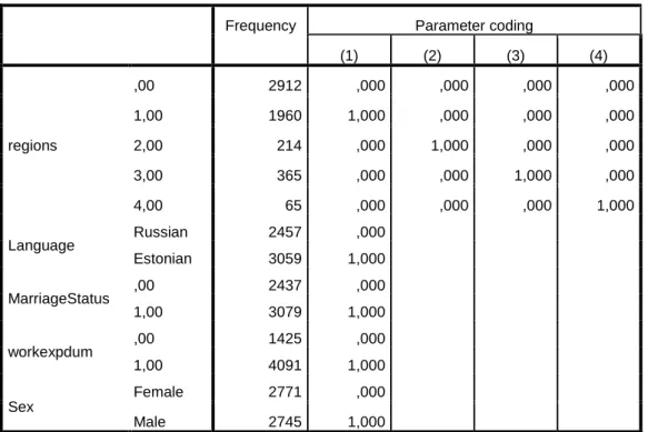
In our model, status variable is dependent variable. Also status variable is binary variable, which is suitable for logistic regression, and it consists of only 0 and 1 inputs. Meaning of “0” is being “Bad Client” who is not likely to pay his/her debt and meaning of “1” is “being Good Client” who is likely to pay his/her debt properly as scheduled. We have 15 variables as our independent variables in our first model such as; sex, age, estate and marriage status… Sex, language, marriage status, work experience and regions are categorical variables and these variables expressed as dummy variables in our model.

Frequency Parameter coding

(1) (2) (3) (4) regions ,00 2912 ,000 ,000 ,000 ,000 1,00 1960 1,000 ,000 ,000 ,000 2,00 214 ,000 1,000 ,000 ,000 3,00 365 ,000 ,000 1,000 ,000 4,00 65 ,000 ,000 ,000 1,000 Language Russian 2457 ,000 Estonian 3059 1,000 MarriageStatus ,00 2437 ,000 1,00 3079 1,000 workexpdum ,00 1425 ,000 1,00 4091 1,000 Sex Female 2771 ,000 Male 2745 1,000

(19)

18 As we see on table, categorical variables consist one or more dummy variables. For example Sex has one dummy variable and being “Male” is represented by “Sex(1)” by IBM SPSS 21. Regions has more than one dummy variables and for example, region number 3 is represented by “Regions(3)”.

Let us see what result shows up when we use all of our variables in our first model.

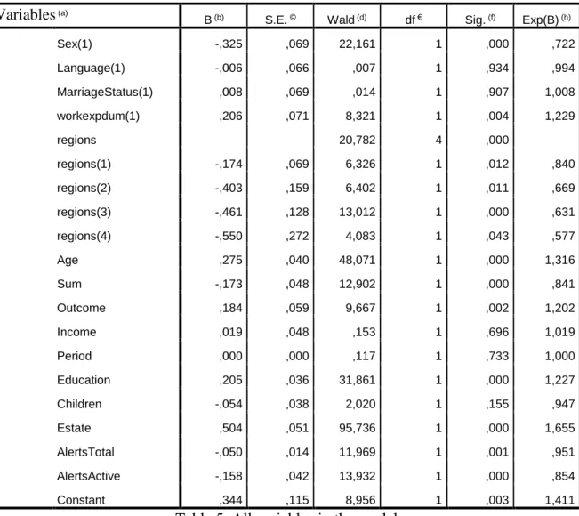
Variables (a)

B (b) _S.E. © _Wald (d) _df € _Sig. (f) _Exp(B) (h)

Sex(1) -,325 ,069 22,161 1 ,000 ,722 Language(1) -,006 ,066 ,007 1 ,934 ,994 MarriageStatus(1) ,008 ,069 ,014 1 ,907 1,008 workexpdum(1) ,206 ,071 8,321 1 ,004 1,229 regions 20,782 4 ,000 regions(1) -,174 ,069 6,326 1 ,012 ,840 regions(2) -,403 ,159 6,402 1 ,011 ,669 regions(3) -,461 ,128 13,012 1 ,000 ,631 regions(4) -,550 ,272 4,083 1 ,043 ,577 Age ,275 ,040 48,071 1 ,000 1,316 Sum -,173 ,048 12,902 1 ,000 ,841 Outcome ,184 ,059 9,667 1 ,002 1,202 Income ,019 ,048 ,153 1 ,696 1,019 Period ,000 ,000 ,117 1 ,733 1,000 Education ,205 ,036 31,861 1 ,000 1,227 Children -,054 ,038 2,020 1 ,155 ,947 Estate ,504 ,051 95,736 1 ,000 1,655 AlertsTotal -,050 ,014 11,969 1 ,001 ,951 AlertsActive -,158 ,042 13,932 1 ,000 ,854 Constant ,344 ,115 8,956 1 ,003 1,411

Table 5. All variables in the model

Briefly, review of table is:

 column (a) shows independents variables into model (In first model we add all variables into model),

 column (b) is Beta coefficients which give main component of regression model,

 (c) is Standard Errors are associated the beta coefficients and standard errors is required to use for estimating confidence intervals,

(20)

19  column (d) provides Wald chi-square test values and column (f) provides two tailed

p-values for each coefficients. Null hypothesis is 𝛽_𝑖 = 0 and alternative hypothesis is

𝛽𝑖 ≠ 0. If p-values is more than 0.05, 0.10, it means we cannot reject null hypothesis. It shows concerned variable is insignificant in model,

 (e) is the degrees of freedom for each of test coefficients,

 column (h) is odds ratios of predictors and these numbers are the exponentiation of the coefficients .

Interpretation of table: There are significant and insignificant variables in our first model. Categorical variable sex, work experience, regions are significant however language variable has 0.934 p-value and it means this variable is not significant when we regard 90%, 95% and 99% significant levels. Age, sum, outcome, education, estate, payment alert total and payment alert active are significant variables. On the other hand, incomes, period, number of children variables have 0.696, 0.733 and 0.155 p-values respectively and none of them are significant when we consider 90%, 95% and 99% significant level. Also it is possible to have further assessment on model by using backward method of SPSS 21. Backward method provides backward elimination which method starts with all variables in the model and eliminates variables step by step that are considered the least significant until all the remaining variable have a p-values below desired significant level. (you can check Annex 1)

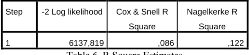
Step -2 Log likelihood Cox & Snell R Square

Nagelkerke R Square

1 6137,819 ,086 ,122

Table 6. R Square Estimates

There are two R² estimates in model summary stable. These are pseudo- R²; meaning is these are analogous to R² in standard multiple regression, but do not carry the same interpretation. The Nagelkerke estimate is calculated in such a way as to be constrained between 0 and 1. So, it can be evaluated as indicating model fit; with a better model displaying a value closer 1. The larger Cox & Snell estimate is better the model; but it can be greater than 1.These metrics should be interpreted with caution, they offer little confidence in interpreting the model fit. [10]

In our case, our Nagelkerke R square is 0.122 and it is not so satisfied number and it is possible to increase the value by adding additional variables into model. For example, we can consider previous researches about credit scoring system related with regression analysis techniques. We can determine which additional parameters should be added to our model. Also – 2 log likelihood is 6137,819, if this value is smaller, it means model would be better.

(21)

20

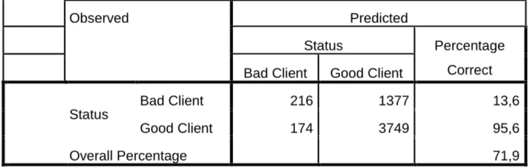
Observed Predicted

Status Percentage

Correct Bad Client Good Client

Status

Bad Client 216 1377 13,6

Good Client 174 3749 95,6

Overall Percentage 71,9

a. The cut value is ,500

Table 7. Classification Table

An intuitively appealing way to summarize the result of fitted logistic regression model is via a classification table. This table is the result of cross-classifying the outcome variable, 𝑦, with a dichotomous variable whose values are derived from the estimated logistic probabilities. In this application the coefficients produced by the model are used for predicting the outcome (in a binary way) rather that for estimating the probability of the event. To obtain the derived dichotomous variable we must define a cut-point and compare each estimated probability to cutoff point. If the estimated probability exceed cutoff point then we let the derived variable be equal to 1; otherwise it is equal to 0. The most commonly used value for cutoff is 0.5. [3]

Needless to say that all the modelling approaches may have errors and it happens in credit risk modeling too. There are two types of error in classification table that we can relate easily with credit scoring:

Error type 1 which means bad credits considered as good one,

Error type 2 which means good credits considered as bad one.

Errors type 1 is likely to cause losing the loan for lender. It may cause to increase risk of bankrupt however error type 2 is likely to cause losing the potentially good customers for bank. So error type 2 is missing opportunities. Our expectation is minimizing these two error types. In our first model, 1377 bad customers predicted as good customer which is error type I and 174 good customers are predicted as bad client which is error type 2.

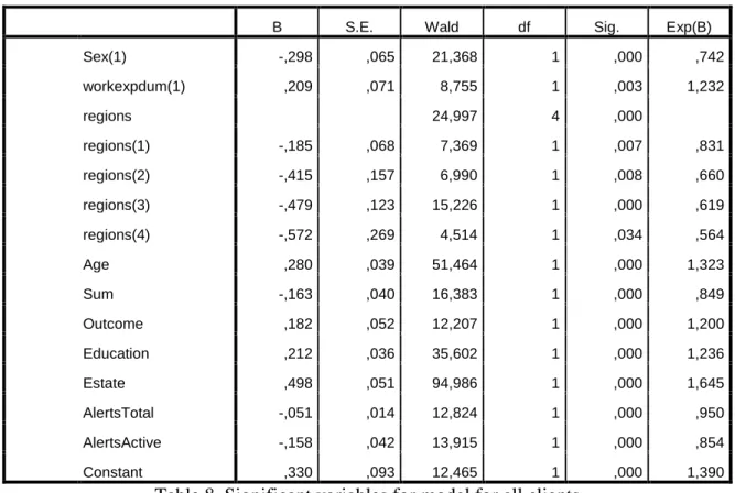
4.2 Final Model After Elimination of Insignificant Variables

Firstly, we added all the variables into model in order to understand which variables are significant and insignificant in our model. To have final model, now we should apply the logistic regression by adding only significant variables. As we observed from 6th step of SPSS backward method output(Annex 1) that we have sex, work experience, regions, age, sum,

(22)

21 outcome, education, estate, payment alert total and payment alert active as our significant independent variables.

B S.E. Wald df Sig. Exp(B)

Sex(1) -,298 ,065 21,368 1 ,000 ,742 workexpdum(1) ,209 ,071 8,755 1 ,003 1,232 regions 24,997 4 ,000 regions(1) -,185 ,068 7,369 1 ,007 ,831 regions(2) -,415 ,157 6,990 1 ,008 ,660 regions(3) -,479 ,123 15,226 1 ,000 ,619 regions(4) -,572 ,269 4,514 1 ,034 ,564 Age ,280 ,039 51,464 1 ,000 1,323 Sum -,163 ,040 16,383 1 ,000 ,849 Outcome ,182 ,052 12,207 1 ,000 1,200 Education ,212 ,036 35,602 1 ,000 1,236 Estate ,498 ,051 94,986 1 ,000 1,645 AlertsTotal -,051 ,014 12,824 1 ,000 ,950 AlertsActive -,158 ,042 13,915 1 ,000 ,854 Constant ,330 ,093 12,465 1 ,000 1,390

Table 8. Significant variables for model for all clients

As we see, coefficients are slightly changed when we include only significant variables into model. In our new model, we can see that sex dummy variable’s coefficient number is -0.298 and it means “male” customer has negative effect on probability of being good customer. If customer have more than 1 year work experience, it contributes positively to being good customer. Also it is easy to see the effects of living in different regions on model. Based category region0 is represent only Harjumaa and customer from Harjumaa has better chance to be good candidate when we compare with other regions. Regions(1) contains; Tartumaa, Pärnumaa, Läänema and Valgamaa have slightly lower chance than Harjumaa region however regions(2) (involves; Ida-Virumaa, Viljandimaa, Järvamaa, and Hiiuma), regions(3) (involves; Raplaama, Lääne-Virumaa and Põlvamaa) and regions(4) (Saaremaa, Võrumaa and Jõgevamaa) have -0,415,-0,479 and -0,572 coefficients values respectively. Moreover, increasing age of customers, outcome, education level and number of estates contributes to increase probability of being good customer. On the other hand, sum, total and active alerts have negative impact. Needless to say that, when borrowed amount of money increases, credit-worthiness decreases at the same time.

(23)

22 𝑙𝑛 ( 𝜋 1 − 𝜋) = 0,330 − 0,298 ∙ 𝑠𝑒𝑥(1) + 0,209 ∙ 𝑤𝑜𝑟𝑘𝑒𝑥𝑝(1) − 0,195 ∙ 𝑟𝑒𝑔𝑖𝑜𝑛(1) − 0,415 ∙ 𝑟𝑒𝑔𝑖𝑜𝑛(2) − 0,479 ∙ 𝑟𝑒𝑔𝑖𝑜𝑛(3) − 0,572 ∙ 𝑟𝑒𝑔𝑖𝑜𝑛(4) + 0,29 ∙ 𝑎𝑔𝑒 − 0,163 ∙ 𝑠𝑢𝑚 + 0,192 ∙ 𝑜𝑢𝑡𝑐𝑜𝑚𝑒 + 0,212 ∙ 𝑒𝑑𝑢𝑐𝑎𝑡𝑖𝑜𝑛 + 0,499 ∙ 𝑒𝑠𝑡𝑎𝑡𝑒 − 0,051 ∙ 𝑡𝑜𝑡𝑝𝑎𝑦𝑎𝑙𝑒𝑟𝑡𝑠 − 0,159 ∙ 𝑎𝑐𝑡𝑝𝑎𝑦𝑎𝑙𝑒𝑟𝑠𝑡𝑠

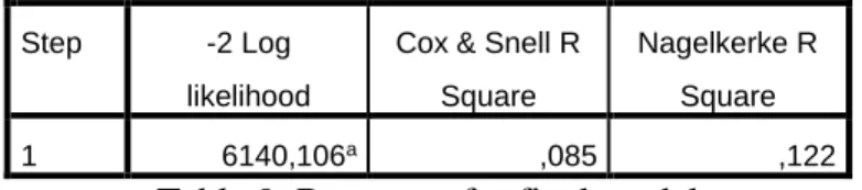
As we can see, Cox & Snell R square has changed slightly (approximately 0,001) and Nagelkerke R square has exactly the same number. Removing insignificant variables from model did not change R square values.

Step -2 Log

likelihood

Cox & Snell R Square

Nagelkerke R Square

1 6140,106a _,085 _,122

Table 9. R squares for final model

Goodness of fit statistics assess the fit of a logistic model against actual outcomes. The goodness of fit test is the Hosmer Lemeshow (H-L) test. This statistics test 𝐻₀ hypothesis of HL test is

𝐻0: 𝐸[𝑌] =

exp ( 𝛽0+ 𝛽1𝑥1+ ⋯ + 𝛽𝑘𝑥𝑘)

1 + exp ( 𝛽0+ 𝛽1𝑥1+ ⋯ + 𝛽𝑘𝑥𝑘)

using chi-square, and if becomes more than 0.05, shows that the model fits well to data.[7] Our p-value is 0.107 and p-value is bigger than 0.05 and in this case, we can say that model fits well enough to data.

Step Chi-square df Sig.

1 13,144 8 ,107

Table 10. Hosmer and Lemeshow Test

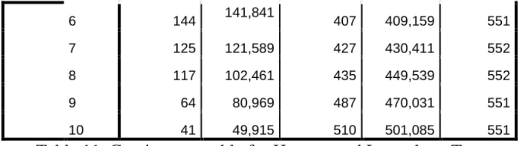
The Contingency Table for Hosmer and Lemeshow Test simply shows the observed and expected values for each category of the outcome variable as used to calculate the Hosmer and Lemeshow chi-square.

Status = Bad Client Status = Good Client Total Observed Expected Observed Expected

1 291 299,097 261 252,903 552

2 231 239,700 321 312,300 552

3 229 209,633 324 343,367 553

4 181 185,120 371 366,880 552

(24)

23 6 144 141,841 407 409,159 551 7 125 121,589 427 430,411 552 8 117 102,461 435 449,539 552 9 64 80,969 487 470,031 551 10 41 49,915 510 501,085 551

Table 11. Contingency table for Hosmer and Lemeshow Test

A model classification table which describes both expected model classifications and actual model classifications. The Hosmer-Lemeshow table divides the data into 10 groups each representing the expected and observed frequency of both 1(Good Client) and 0(Bad Client) values. The expected frequency of data assigned to each deciles should match the actual frequency outcome and each deciles should contain data. [12]

Observed Predicted

Status Percentage

Status

Bad Client 216 1377 13,6

Table 12. Classification table

Classification table has almost same figures as classification table of our first model. Removing insignificant variables from model did not change the percentage of correct predictions. 71.9 percent of correct predictions may be acceptable as satisfying result however 1377 bad clients interpreted as good client which is increasing the risk of bankrupt (error type1). And we foresighted approximately only 14 percent of bad clients correctly (specificity) but needless to say that rejected borrowers by bank are not part of training dataset and proportion of clients are not equal (number of good clients is almost 3 times bigger). 95.6 percentage of correct predictions for good clients (sensitivity) is sufficiently high but 173 potential good customers are predicted as bad clients which shows that missing opportunities (error type 2).

Another point that can confirm the result of logit modelling is relative operating characteristic (ROC) curve, which shows a receiver operating characteristics and used for evaluating the logistic model as well. The ROC plot is merely the graph of points defined by sensitivity and 1-specificity. Customarily, sensitivity takes the y-axis and 1-specificity takes the x-axis. If the area under the curve becomes maximum amount, then the model fits data well. [7] The area

(25)

24 under the ROC curve, which ranges from 0.5 to 1.0, provides a measure of the model’s ability to discriminate between outcomes. [3]

Figure 4. ROC Curve

SPSS outputs show that area under the curve is 0,685 with 95 percent of confidence interval (lower bound is 0,670 and upper bound is 0,700). Also the area under the curve has 0.00 p-value. It is significant and it means that logistic regression classifies the group significantly better than by chance.

Test Result Variable(s): Predicted probability

Area Std. Errora _{Asymptotic Sig.}b _{Asymptotic 95% Confidence}

Interval

Lower Bound Upper Bound

,685 ,008 ,000 ,670 ,700

Table 13. Area under the curve

Decision of cutting point is also important and it depends on policies of lenders. They would prefer to take increasing risk of bankrupt while they add new customers or they would prefer to decrease the risk of bankrupt while they lose potentially good clients. In this project, our goal

(26)

25 was having maximum percentage of correct prediction from classification table. And as we can observe from table below that best cut-off point is 0.50 in order to have higher percentage of correct predictions. Classification Table Cut-off points Bad Client Error Type I Error Type II Good Client Percentage Correct 0,3 10 1583 2 3921 71,3% 0,4 50 1543 34 3889 71,4% 0,45 114 1479 78 3845 71,8% 0,5 216 1377 173 3750 71,9% 0,55 355 1238 338 3585 71,4% 0,6 537 1056 603 3320 69,9% 0,7 995 598 1422 2501 63,4% 0,8 1386 207 2539 1384 50,2%

Table 14. Classification table for different cut-off points

Additionally alternative way to decide cut-off point is considering specificity and sensitivity table (Annex 2). According to table, cut-off point is 0,701 with 0,633 sensitivity and 0,367 1-specifity. This approach provides balanced result which has 63 percentage of correct prediction for good and bad clients separately.

Figure 5. Sensitivity and specificity graph

0,000 0,100 0,200 0,300 0,400 0,500 0,600 0,700 0,800 0,900 1,000 0,0000000 ,4288409 ,4788519 ,5140724 ,5452682 ,5691461 ,5876790 ,6086687 ,6257283 ,6427761 ,6601172 ,6765096 ,6921858 ,7069751 ,7213207 ,7350054 ,7488629 ,7617 50 2 ,7760219 ,7882555 ,8025090 ,8167066 ,8298785 ,8466673 ,8620953 ,8806964 ,9031497 ,9309293

Cut off Point

(27)

26

5 Segmentations/Models for 4 Different Age Groups

Following overview is based on [6]

In some cases, using several scorecards for a portfolio provides better risk differentiation than using one scorecard on everyone. This is usually the case where a population is made up of distinct subpopulations, and where one scorecard will not work efficiently for all of them (i.e., we assume that different subpopulations in our portfolio). The process of identifying these subpopulations is called segmentation. There are two main ways in which segmentation can be done:

1. Generating segmentation ideas based on experiences and industry knowledge, and then validating these ideas using analytics

2. Generating unique segments using statistical techniques such as clustering or decision trees.

In either case, any segments selected should be large enough to enable meaningful sampling for separate scorecard development. Segments that exhibit distinct risk performance, but have insufficient volume for separate scorecard development, can still be treated differently using different cut-offs or other strategy considerations.

Segmentation, whether using experience or statistical methods, should also be done with future plans in mind. Most analysis and experience is based on the past, but scorecards need to be implemented in the future, on future applicant segments. One way to achieve this is by adjusting segmentation based on, for example, the organization’s intended target market. Traditionally, segmentation has been done to identify an optimum set of segments that will maximize performance—the approach suggested here is to find a set of segments for which the organization requires optimal performance, such as target markets. This approach underscores the importance of trying to maximize performance where it is most needed from a business perspective and ensures that the scorecard development process maximizes business value. This is an area where marketing staff can add value and relevance to scorecard development projects.

(28)

27 • Demographics. Regional (province/state, internal definition, urban/rural, postal-code based, neighbourhood), age, lifestyle code, time at bureau, tenure at bank

• Product Type. Gold/platinum cards, length of mortgage, insurance type, secured/unsecured, new versus used leases for auto, size of loan

• Sources of Business (channel). Store-front, take one, branch, Internet, dealers, brokers • Data Available. Thin/thick (thin file denotes no trades present) and clean/dirty file (dirty denotes some negative performance) at the bureau, revolver/transactor for revolving products, SMS/voice user

• Applicant Type. Existing/new customer, first time home buyer/mortgage renewal, professional trade groups (e.g., engineers, doctors,etc.)

• Product Owned. Mortgage holders applying for credit cards at the same bank.

In our study, we will create 4 different segmentation groups based one age independent variable. Age variable has 4 subgroups; clients who are “30 years old and younger than 30”, clients “between 31 and 45”, “clients between 45 and 60” and “clients who are older than 60 years old”. These groups have 1553, 2244, 1453 and 341 observations respectively.

Frequency Percent

30 And Younger Than 30 Years Old ₁₅₅₃ _27,8 Older Than 30 And Younger Than 46 2244 40,1 Older Than 45 And Younger Than 60 1453 26,0 Older Than 60 Years Old 341 6,1

Total 5591 100,0

Table 15. Age groups

5.1 Model for 30 And Younger Than 30 Years old Clients

We have 1553 clients who are 30 and younger than 30 years old however 1531 of clients in analysis because 22 of them are missing cases.

(29)

28

Unweighted Casesa _N _Percent

Selected Cases Included in Analysis 1531 98,6 Missing Cases 22 1,4 Total 1553 100,0 Unselected Cases 0 ,0 Total 1553 100,0

Table 16. Case summary

Result shows quite different model if we compare with our final model without segmentation. Regions, outcome, income, education and total alerts are significant. Language is also significant with 90% of significance level. Output shows us that clients whose mother tongue is Estonian are likely to be more trustworthy borrowers. Needless to say, number of total alerts has negative effect on creditworthiness as we can foresee. Number of estate and higher education are contributing to be good customer.

Language(1) ,199 ,117 2,918 1 ,088 1,221 regions 33,162 4 ,000 regions(1) -,488 ,132 13,690 1 ,000 ,614 regions(2) -,746 ,212 12,336 1 ,000 ,474 regions(3) -,936 ,343 7,455 1 ,006 ,392 regions(4) -1,339 ,498 7,217 1 ,007 ,262 Outcome ,297 ,113 6,921 1 ,009 1,345 Income -,161 ,077 4,413 1 ,036 ,851 Education ,257 ,060 18,191 1 ,000 1,293 Estate ,408 ,120 11,501 1 ,001 1,504 AlertsTotal -,087 ,026 10,966 1 ,001 ,917 Constant ,362 ,159 5,196 1 ,023 1,437

Table 17. Variables into model for first age group And in this age group, model for probability of being good customer is:

ln ( 𝜋

1 − 𝜋) = 0,362 + 0,199 ∙ 𝑙𝑎𝑛𝑔𝑢𝑎𝑔𝑒(1) − 0,488 ∙ 𝑟𝑒𝑔𝑖𝑜𝑛(1) − 0.746 ∙ 𝑟𝑒𝑔𝑖𝑜𝑛(2) − 0,936 ∙ 𝑟𝑒𝑔𝑖𝑜𝑛(3) − 1,339 ∙ 𝑟𝑒𝑔𝑖𝑜𝑛(4) + 0,297 ∙ 𝑜𝑢𝑡𝑐𝑜𝑚𝑒 − 0,161 ∙ 𝑖𝑛𝑐𝑜𝑚𝑒 + 0,257 ∙ 𝑒𝑑𝑢𝑐𝑎𝑡𝑖𝑜𝑛 + 0,408 ∙ 𝑒𝑠𝑡𝑎𝑡𝑒 − 0,087 ∙ 𝑡𝑜𝑡𝑝𝑎𝑦𝑎𝑙𝑒𝑟𝑡𝑠

Model provides 62.4 percentage of correct predictions when cut-off point is 0.5. Good clients are well predicted however correct prediction for bad clients are low and around 29 percentage.

(30)

29

Observed Predicted

Status Percentage

Status

Bad Client 183 440 29,4

There are some classification results when we determined some specific different cut-off points. It is possible to get better result when cut-off point is 0.55 than our cut-off point is 0.5.

Classification Table Cut-off points Bad Client Error Type I Error Type II Good Client Percentage Correct 0,3 15 608 4 904 60% 0,4 64 559 28 880 61,7% 0,5 183 440 136 772 62,4% 0,55 272 351 210 698 63,4% 0,6 381 242 383 525 59,2% 0,7 549 74 714 194 48,5%

SPSS outputs shows that area under the curve is 0,636 with 95 significance level (lower bound is 0,608 and upper bound is 0,665). Also the area under the curve has 0.00 p-value. It express that logistic regression classifies the group significantly better than by chance.

(31)

30 Figure 6. Roc Curve

Area Std. Error Asymptotic Sig. Asymptotic 95% Confidence Interval

,636 ,014 ,000 ,608 ,665

5.2 Model For Between 31 To 45 Years Old

Let us check the next age group which is consist of clients who are older 30 years old and younger than 46 years old. We have 2244 clients in this age group however 1.3 percent of clients is missing cases. 2215 of clients is included in analysis.

(32)

31

Unweighted Cases N Percent

We have 8 significant variables in our model. These variables are sex, work experience, region, outcome, period, education level, number of estates and active alerts. Having more than one year work experience is contributing creditworthiness positively. Moreover client who have higher education level and number of estates or ownership of estate(s) are increasing probability of being good customer. On the other hand, active alerts is reducing the probability of being good customer. Also period has negative effect too and we can say that longer instalment period reduces chance to be good client for candidate. Coefficient of period is so small because of scale problem. Additionally, female candidates are more reliable clients than man in this age group.

Sex(1) -,343 ,102 11,256 1 ,001 ,710 workexpdum(1) ,349 ,116 9,143 1 ,002 1,418 regions(1) -,643 ,271 5,619 1 ,018 ,526 Outcome ,177 ,074 5,709 1 ,017 1,194 Period -,001 ,000 4,203 1 ,040 ,999 Education ,228 ,056 16,809 1 ,000 1,256 Estate ,535 ,076 50,086 1 ,000 1,707 AlertsActive -,236 ,059 15,698 1 ,000 ,790 Constant ,284 ,148 3,688 1 ,055 1,329

Table 22. Variables in the equation for second age group

Clients who live in Põlvamaa and Viljandimaa are to reduce probability of being customer. Living in rest of countries provides candidates some benefits in this age group model. This age group’s specific model is simpler and plainer than previous models and model for probability of being good customer is:

ln ( 𝜋

1 − 𝜋) = 0,284 − 0,343 ∙ 𝑠𝑒𝑥(1) − 0,643. 𝑟𝑒𝑔𝑖𝑜𝑛(1) + 0,177 ∙ 𝑜𝑢𝑡𝑐𝑜𝑚𝑒 − 0,001 ∙ 𝑝𝑒𝑟𝑖𝑜𝑑 + 0,228 ∙ 𝑒𝑑𝑢𝑐𝑎𝑡𝑖𝑜𝑛 + 0,535 ∙ 𝑒𝑠𝑡𝑎𝑡𝑒 − 0,236 ∙ 𝑎𝑐𝑡𝑝𝑎𝑦𝑎𝑙𝑒𝑟𝑡𝑠

(33)

32 Model in this age group provides 72.1 percentage of correct predictions when cut-off point is 0.5. Good clients are predicted with 97.7 percentage correctly however model is not successful to predict bad clients efficiently and percentage of correct predictions is very low.

Observed Predicted

Status Percentage

Status

Bad Client 43 583 6,9

Also there are some specific off points and percentage of correct predictions for these cut-off points. Highest percentage of correct predictions in classification table is 0.5 in this specific age group. It is possible to increase percentage of correct prediction for bad clients’ predictions however it has negative impact on general model which decreases percentage of correct prediction dramatically. Classification Table Cut-off points Bad Client Error Type I Error Type II Good Client Percentage Correct 0,4 14 612 12 1577 71,8% 0,45 25 601 23 1566 71,8% 0,5 43 583 36 1553 72,1% 0,55 84 542 84 1505 71,7% 0,6 146 480 180 1409 70,2% 0,7 375 251 582 1007 62,4%

Area under the curve is 0,664 with 95 significance level and confidence interval lower bound is 0,639 and upper bound is 0,688. If area under the curve is between 0.6 and 07, we can say it is on acceptable level. Also the area under the curve has 0.00 p-value. It expresses that logistic regression classifies the group significantly better than by chance.

(34)

33 Figure 7. ROC Curve

,664 ,012 ,000 ,639 ,688

5.3 Model For Between 46 To 60 Years Old

In this study, we have 1453 clients who are between 46 and 60 years old. 19 of them are missing value and they are excluded. 1434 clients are included in analysis.

Unweighted Cases N Percent

(35)

34 Let us check the output. Model have 8 significant variables. Language dummy variable is part of model when we consider 90% significance level but it is possible to exclude it when we take significance level 95%. Significant variables are sex, language, region, sum, income, education, estate and active alerts. Result shows us that female customers are more reliable than men customers in this age group like previous one. Also it is easy to see that living in different countries have impact on being good customer. Amount of borrowed money is also important. It trigger bigger risk to pay it back while amount of sum is increasing. Higher education level and number of estates are contributing to be good customer. Customer, who have higher education level and have his/her own estate, is likely to be more trustworthy candidate.

Sex(1) -,376 ,141 7,080 1 ,008 ,686 Language(1) -,264 ,143 3,382 1 ,066 ,768 regions 14,494 2 ,001 regions(1) -,577 ,210 7,542 1 ,006 ,562 regions(2) -1,317 ,463 8,092 1 ,004 ,268 Sum -,264 ,089 8,832 1 ,003 ,768 Income ,219 ,093 5,568 1 ,018 1,244 Education ,175 ,083 4,447 1 ,035 1,191 Estate ,447 ,088 25,982 1 ,000 1,563 AlertsActive -,265 ,078 11,403 1 ,001 ,767 Constant 1,032 ,207 24,769 1 ,000 2,808

Table 27. Variables in the model

And in this age group, the model looks like this:

𝑙𝑛 ( 𝜋

1 − 𝜋) = 1,032 − 0,376 ∙ 𝑠𝑒𝑥(1) − 0.264 ∙ 𝑙𝑎𝑛𝑔𝑢𝑎𝑔𝑒 − 0,577 ∙ 𝑟𝑒𝑔𝑖𝑜𝑛(1) − 1,317 ∙ 𝑟𝑒𝑔𝑖𝑜𝑛(2) − 0,264 ∙ 𝑠𝑢𝑚 + 0,219 ∙ 𝑒𝑑𝑢𝑐𝑎𝑡𝑖𝑜𝑛 + 0,447 ∙ 𝑒𝑠𝑡𝑎𝑡𝑒 − 0,265 ∙ 𝑎𝑐𝑡𝑝𝑎𝑦𝑎𝑙𝑒𝑟𝑡𝑠

Logistic regression model provides 79.6 percent of correct prediction when cut-off point is 0.5. Good clients are well predicted with 99 percentage however bad clients is predicted with only 5 percentage.

(36)

35

Observed Predicted

Status Percentage

Status

Bad Client 14 282 4,7

Table 28. Classification Table

As we can see on classification table below, current cut-off point provides higher percentage of correct predictions than other cut-off points. It is possible to increase percentage of correct predictions to determine bad clients if we pick higher cut-off point however unfortunately it causes another problem which will effect on general percentage of correct prediction sharply.

Classification Table Cut-off points Bad Client Error Type I Error Type II Good Client Percentage Correct 0,4 7 289 4 1134 79,5 0,45 8 288 6 1132 79,5 0,5 14 282 11 1127 79,6 0,55 15 281 17 1121 79,2 0,6 27 269 38 1100 78,6 0,7 85 211 116 1022 77,2

Area under the curve is 0,681 with 95 significance level and confidence interval for lower bound is 0,647 and upper bound is 0,715. Area under the curve is around 0.7. We can say that model has ability to discriminate between two outcomes. It is possible to interpret the area under the curve is good enough when it is around 0.7. Also the area under the curve has 0.00 p-value. It means that logistic regression classifies the group significantly better than by chance.

(37)

36 Figure 8. ROC curve

,681 ,017 ,000 ,647 ,715

5.4 Model For Older Than 60 Years Old Clients

There are 341 clients who are older than 60 years old. Model includes 336 of them because of 5 of them have missing values. Logistic regression requires complete data without missing cases. Therefore we excluded missing cases.

(38)

37

Unweighted Casesa _N _Percent

We have the simplest and the plainest model in this age group and the latest model has only 4 significant variables. These variables are region, sum, number of estates and total alerts respectively. It is easy to see that if client demand to borrow bigger amount of money, it will increase the risk of paying debt back and it will decrease creditworthiness of candidate in our model for this age group. Needless to say that total alerts have negative impact as we can presume.

regions(1) -2,698 1,048 6,627 1 ,010 ,067

Sum -,671 ,224 8,933 1 ,003 ,511

Estate 1,228 ,311 15,605 1 ,000 3,413

AlertsTotal -,317 ,100 10,116 1 ,001 ,728

Constant 4,371 1,063 16,890 1 ,000 79,100

Table 32. Variables in the model

Also we can see that region variable is important indicator. Living in Jõgevamaa, Läänemaa, Põlvamaa, Valgamaa, Võrumaa and Tartumaa are contributing more to be good customer than other countries in this age group which is consisted of clients who are older than 60 years old.

And the model is as follows:

ln ( 𝜋

1 − 𝜋) = 4,371 − 2,698 ∙ 𝑟𝑒𝑔𝑖𝑜𝑛(1) − 0,671 ∙ 𝑠𝑢𝑚𝑠 + 1,228 ∙ 𝑒𝑠𝑡𝑎𝑡𝑒 − 0,317 ∙ 𝑡𝑜𝑡𝑝𝑎𝑦𝑎𝑙𝑒𝑟𝑡𝑠

Classification table shows us that model provides 86.2 percent of correct predictions when cut-off point is 0.5. 291 of 293 good clients are predicted correctly (99.3%) however bad clients are predicted with only 6.3 percentage. Therefore model is able to predict 3 of 48 bad clients correctly.

(39)

38

Observed Predicted

Status Percentage

Status

Bad Client 3 45 6,3

According to classification table below, we can say that model provides 87.1 percentage of correct predictions when cut-off point is 0.6 which gave better result than when cut-off point is 0.5. Classification Table Cut-off points Bad Client Error Type I Error Type II Good Client Percentage Correct 0,4 0 48 1 292 85,6% 0,45 2 46 2 291 85,9% 0,5 3 45 2 291 86,2% 0,55 6 42 4 289 86,5% 0,6 12 36 8 285 87,1% 0,7 17 31 13 280 87,1% 0,75 28 20 44 249 81,2%

Area under the curve is 0,775 and confidence interval with 95 significance level is from 0,699 to 0,851. Since area under the curve is between 70% and 80%, it is a good model. Moreover we can say that ability of a fitted model to discriminate between two outcomes is on fairly acceptable level. Also, the area under the curve has 0.00 p-value. It means that logistic regression classifies the group significantly better than by chance.

(40)

39 Figure 9. ROC curve

Area Under the Curve

,775 ,039 ,000 ,699 ,851

(41)

40

6 Results

Firstly, we created one model for all clients without any separation which the model is created by logistic regression and according to our model, sex, work experience, regions, age, sum, outcome, education, estate, total alerts and active alerts are significant variables and model provided 71.9% of correct prediction overall when cut-off point is 0.5.

In second part, we separated clients regarding their age groups in order to have different credit scoring model for different age group. Purpose of creating different models for each group is observing whether it helps increasing percentage of correct prediction or not which may be dramatically critical in real life for lenders. Therefore we divided data four different subgroups regarding each age groups and we created 4 different models for each age groups. These are clients who are 30 years old and younger, clients who are between 31 and 45 years old, clients who are between 46 and 60 years old and clients who are older than 60 years old respectively. In first model for age groups, significant variables are language, region, outcome, income, education, estate and total alerts and model provided 63.4% of correct predictions. Second model for age groups have 8 significant variables; sex, work experience, region, outcome, period, education, estate and active alerts. Second segmentation age group provided 72.1% of correct prediction. Next model have sex, language, regions, sum, income, education, estate and active alerts as significant independent variables which provides 79.6% of correct prediction. Last model for age groups has only 4 significant variables; region, sum, estate and total alerts and clients is predicted with 87.1% correctly by this model.

Classification Table Cut-off points Bad Client Error Type I Error Type II Good Client Percentage

Final Model (one model) 0,5 216 1377 173 3750 71,9%

30 and Younger 0,55 272 351 210 698 63,4%

Between 31 to 45 0,5 43 583 36 1553 72,1%

Between 46 to 60 0,5 14 282 11 1127 79,6%

Older than 60 0,6 12 36 8 285 87,1%

4 Segmentation models together 341 1252 265 3663 72,5%

Table 36. Model comparison between model for all clients and segmentation

We predicted 72.5% of our clients correctly with helps of segmentation regarding age variable. And as we mentioned before, only one model for all clients provided 71.9% of correct prediction. Segmentation helped to increase correct predictions from 71.9% to 72.5% and it is equal to additionally 38 correctly predicted customers in our study. Error type I decreased from

(42)

41 1377 to 1252 and it implies that number of bad customers considered as good customer which cause to rise risk of bankrupt and frauds. On the other hand, it caused to increase error type II from 173 to 265 which implies that number of client who are actually good but we considered as bad clients.