CDO pricing using single factor MG-NIG copula model with stochastic correlation and random factor loading

(1)

Contents lists available atScienceDirect

Journal of Mathematical Analysis and Applications

www.elsevier.com/locate/jmaa

CDO pricing using single factor

M

_G

_-

_{N I}

_G

copula model with stochastic

correlation and random factor loading

Ruicheng Yang

a,b,∗

, Xuezhi Qin

a

, Tian Chen

a

a_{Postdoctor Working Station of School of Management, Dalian University of Technology, Linggong Road No. 2, Dalian 116024, Liaoning, PR China} b_{School of Mathematics and Information, Ludong University, Yantai 264025, PR China}

a r t i c l e i n f o a b s t r a c t

Article history:

Received 29 September 2007 Available online 4 September 2008 Submitted by J.A. Filar

Keywords:

MG-N IGcopula model CDO

Stochastic correlation Random factor loadings Loss distribution

We consider the valuation of CDO tranches with single factor MG-N IG copula model,

where the involved distributions are mixtures of Gaussian distribution and_{N I}G distri-bution. In addition, we consider two cases for stochastic correlation and random factor loadings instead of constant factor loadings. We analyze the unconditional characteristic function of accumulated loss of the reference portfolio, and derive the loss distribution through the fast Fourier transform. Moreover, using the loss distribution and semi-analytic approach, we can get the CDO tranches spreads.

1. Introduction

In recent years, collateralized debt obligations (CDOs) were probably the most important type of multi-name credit derivatives. A CDO consists of a portfolio of reference entities (e.g. bonds, loans, residential and commercial mortgages) whose credit risk is sold to investors who, in return for an agreed payment (usually a periodic fee), will bear the losses of the portfolio derived from the default of the reference entities. Through a securitization technique, CDOs repackage a portfolio credit risk into tranches according to credit risk. During the life of the transaction the resulting losses affect ﬁrst the so-called equity piece and then, after the equity tranche has been exhausted, the mezzanine tranches. Further losses, due to credit events on a large number of reference entities, are supported by senior and super senior tranches. The credit risk of the portfolio underlying the CDO is sold in these tranches. Generally, a tranche is deﬁned by a lower attachment point KL and an upper detachment pointKU. The buyers of the tranche

[

KL

,

KU

]

will bear all losses of the portfolio value

in excess of KL and up toKU percent of the initial value of the portfolio. CDO trenching allows the holders of each tranche

to limit their loss exposure to KU

−

KL percent of the initial portfolio value.

The base for pricing CDO tranches is to model the default losses in portfolio of all reference entities. Since it is a well-known fact that defaults appear in all entities and so cannot be treated as independent random events, then, we must ﬁnd an eﬃcient approach to solve this. A common technique for the description of codependence of defaults is to specify a copula that governs the joint distribution of default times, and many cases can be found in [1,2]. More precisely, the copula methodology will help us model the dependency between the default-correlation entities, and many works have proved the factor copula approach is a powerful tool for pricing CDOs within a semi-analytical framework, see [3,4]. However, there still exists a correlation smile behavior in calculating the correlations that are implied by the market prices of tranches. The main explanation of this phenomenon is the lack of tail dependence of the Gaussian copula. Then, various authors have proposed

*

Corresponding author at: Postdoctor Working Station of School of Management, Dalian University of Technology, Linggong Road No. 2, Dalian 116024, Liaoning, PR China.

E-mail address:[email protected](R. Yang).

(2)

different approaches to bring more tail dependence into the model. One approach is the introducing stochastic correlation (see [5,6]) or stochastic risk exposure (see [7]). The risk exposures may or not be associated with a factor structure and may or may not be factor dependent. When the correlation is stochastic and independent of the factor, we will consider a stochastic correlation model. When the correlation depends upon the factor, we will discuss a local correlation model with random factor loadings (see [7]). Meanwhile, many other authors proposed different approaches to use a copula that exhibits more tail dependence: Examples are the

α

-stable copula in Claudio Ferrarese [8], Marshall-Olkin copula in Andersen and Sidenius [7], the doublet distribution in Hull and White [2], and normal inverse Gaussian distribution in [9]. Recently, Geng Xu [10] used the mixture copula model of multi-Gaussian distributions and Dezhong Wang [11] used double mixture of t and Gaussian copula to price the CDO tranches, and they found these mixture copula models ﬁtted better than the previous models, however, they did not consider the stochastic correlation and random factor loadings. Motivated by these mixture copula models, we combine the normal inverse Gaussian (

N I

G) distribution with Gaussian distribution, construct an

M

G-N IG copula model, in addition, for solving the dynamic correlation, we consider stochastic correlation and random

factor loadings.

The paper is organized as follows. Section 2 gives a semi-analytic approach for pricing CDO tranche. Section 3 presents

M

G-N IG copula model. Sections 4 and 5 discuss the

M

G-N IG copula model where that factor loadings are the stochastic

correlation and random factor loadings, respectively. 2. Semi-analytic approach for pricing CDO tranches

For pricing a CDO tranche, that is, ﬁnding the fair spreads of the tranche, we must analyze the values of two legs, default leg (DL) and premium leg (PL) using semi-analytic approach. The value of DL presents the value of tranche losses triggered by credit events during the CDO lifetime, and the value of PL is the premium payments weighted by the outstanding asset (original tranche amount minus accumulated losses). Under the risk-neutral measure, the expected value of both legs should be equal, applying this we can derive the fair spread Sof tranche

[

KL

,

KU

]

, i.e.

S

=

E

[

DL[KL,KU]

]

E

[

PL_[KL,KU]

]

.

(1)

Now let us describe the method to calculate DL and PL for CDO tranche

[

KL

,

KU

]

in detail. For convenience, we assume

the reference portfolio consists ofnentities, and introduce the following notations:

•

Ri—the recovery rate of theith reference entity;

•

Mi—the notional of theith reference entity;

•

Vi—the asset value of theith reference entity;

•

Ai—the lower default barrier of theith reference entity;

• τ

i—the default time of theith reference entity, i.e.,

τ

i

:=

inf

{

t

0: Vi

Ai

}

;

•

T—the maturity time;

•

r—the risk-free discount rate (r

>

0).

Lettingli

:=

Mi

(

1

−

Ri

)

, then accumulated loss at timet is given by:

L

(

t

)

=

n

i=1 Mi

(

1

−

Ri

)

1{τit}

=

n

i=1 li1{τit}

,

(2)

and the aggregate tranche loss of

[

KL

,

KU

]

is:

L_[Kl,KU]

(

t

)

=

min

L

(

t

),

KU

−

min

L

(

t

),

KL

.

(3)

For the default leg, let us assume that

0

t0

<

t1

<

· · ·

<

tM−1

<

tM

=

T (4)

denote the spread payment dates. Now we derive the following results:

Theorem 2.1.Under the risk-neutral probability measure, the price S of CDO tranche

[

KL

,

KU

]

is given by

S

=

E

[

M m=1e−rtm

(

L[KL,KU]

(

tm

)

−

L[KL,KU]

(

tm−1

))

]

E

[

_mM₌₁

tme−rtm_min

{

_max

[

_K_U

−

_L_[_K L,KU]

(

tm

),

0

]

,

KU

−

KL

}]

.

(5)

Proof. First, the expected value of the default leg of the tranche

[

KL

,

KU

]

with respect to the risk neutral probability

(3)

E

[

DL_[KL,KU]

] =

tM

t0 e−rtu_{dE L} [KL,KU]

(

u

)

=

E

_M

m=1 e−rtm

_L [KL,KU]

(

tm

)

−

L[KL,KU]

(

tm−1

)

.

(6)

Second, the expected value of the premium leg of tranche

[

KL

,

KU

]

is the present value of all expected spread payments,

and it is calculated by E

[

PL_[KL,KU]

] =

E

_M

m=1 S

tme−rtmmin

max

KU

−

L[KL,KU]

(

tm

),

0

,

KU

−

KL

,

(7) where

tm

=

tm

−

tm−1.

Substituting (6) and (7) into (1) yields the conclusion (5).

2

Remark 2.1.Eq. (5) shows, the key issue for pricing the CDO tranche

[

KL

,

KU

]

is to ﬁnd the distribution of the accumulated

lossL_[KL,KU]

(

tm

)

of a CDO portfolio. In the following sections we will present the

M

G-N IG copula model, and analyze the

probability distribution ofL

(

t

)

.

3. Single factor

M

G-N IGcopula model

Before giving the single factor

M

G-N IG copula model, let us consider the

N I

G distribution (see [8,9]) and

M

G-N IG

distribution.

Deﬁnition 3.1(

N I

G distribution).The

N I

Gdistribution (normal inverse Gaussian distribution) is a mixture of normal and inverse Gaussian distribution. A random variableU follows a

N I

Gdistribution with parameters

α,

β

,

μ

and

δ

if its density function is of the form

f_{N I}G

(

x

;

α

, β,

μ

, δ)

=

δ

α

exp

(δ

γ

+

β(

x

−

μ

))

π

δ

2

₊

₍

_x

₋

_μ

₎

2 K1

α

δ

2

₊

₍

_x

₋

_μ

₎

2

_,

₍₈₎ whereK1

(

w

)

:=

12

∞ 0 exp

(

−

1 2w

(

t

+

t−1

))

dt, 0

|

β

|

<

α

and

δ >

0.

We denote the

N I

Gdistribution by

N I

G

(

α

, β,

μ

, δ)

. If a random variableU

∼

N I

G

(

α

, β,

μ

, δ)

, then,

E

[

U

] =

μ

+

δ

β

γ

,

Var

[

U

] =

δ

α

2

γ

3

,

(9)

where

γ

:=

α

2

₋

_β

2

_.

Proposition 3.1.The main properties of the

N I

G distribution class are the scaling property U

∼

N I

G

(

α

, β,

μ

, δ)

⇒

cU

∼

N I

G

α

c

,

β

c

,

c

μ

,

c

δ

for c

∈

R

,

(10)

and the stability under convolution for independent random variables U1and U2

U1

∼

N I

G

(

α

, β,

μ

1

, δ

1

)

and U2

∼

N I

G

(

α

, β,

μ

2

, δ

2

)

⇒

U1

+

U2

∼

N I

G

(

α

, β,

μ

1

+

μ

2

, δ

1

+

δ

2

).

(11) Proof. See [9].

2

Deﬁnition 3.2(

M

G-N IGdistribution).The

M

G-N IGdistribution is a mixture distribution of Gaussian distribution and

N I

G

distribution, and a random variable X

∼

M

G-N IG

(

0

,

1

;α

, β,

μ

, δ

;

p

)

is given by

X

=

U

,

with probability 1

−

p

,

V

,

with probability p

,

(12)

whereU

∼

N I

G

(

x

;α

, β,

μ

, δ)

, V is a random variable that followed a standard Gaussian distribution, and p

∈

(

0

,

1

)

is the proportion of the Gaussian component in the mixture distribution X,

α,

β

,

μ

and

δ

is deﬁned as in Deﬁnition 3.1. Denote the probability density function of X by f_M_G_{-N I}_G

(

x

;

0

,

1

;α

, β,

μ

, δ

;

p

)

, then

f_M_G_{-N I}_G

(

x

;

0

,

1

;α

, β,

μ

, δ

;

p

)

=

√

p 2πexp

−

x2 2

+

(

1

−

p

)

f_{N I}G

(

x

;α

, β,

μ

, δ).

(13)

(4)

Deﬁnition 3.3(Single factor

M

G-N IGcopula model).Suppose that the ith asset valueVi of the reference entities is given by

Vi

=

ρ

iY

+

1

−

ρ

2

i

,

i

=

1

, . . . ,

n

,

(14)

where the factor loadings

ρ

i, i

=

1

, . . . ,

n, is a constant and takes values in

[

0

,

1

]

,Y is the common factor of the market,

i,i

=

1

, . . . ,

n, is the idiosyncratic factor of the ith reference entity, and we assume that Y and

i are independent with

random variables with

Y

∼

M

G-N IG

0

,

1

;

α

, β,

−

β

γ

2

α

2

,

γ

3

α

2

;

p

,

(15)

i

∼

M

G-N IG

0

,

1

;

1

−

ρ

2 i

ρ

i

α

,

1

−

ρ

2 i

ρ

i

β,

−

1

−

ρ

2 i

ρ

i

β

γ

2

α

2

,

1

−

ρ

2 i

ρ

i

γ

3

α

2

;

p

,

i

=

1

, . . . ,

n

.

(16)

We call the model given by (14)–(16)single factor

M

G-N IGcopula model.

4. Stochastic correlation

Now we introduce the stochastic correlation into the above

M

G-N IG copula model, and present theith asset value as

follows: Vi

=

ρ

iY

+

1

−

ρ

2 i

i

,

i

=

1

, . . . ,

n

,

(17) where

i

∼

M

G-N IG

(

0

,

1

;

1−ρ2 i ρi

α

,

1−ρ2 i ρi

β,

−

1−ρ2 i ρi

β

γ2 α2

,

1−ρ2 i ρi γ3

α2

;

p

)

, i

=

1

, . . . ,

n, Y is given as in Section 3, all these

being jointly independent,

ρ

iare some random variables taking values in

[

0

,

1

]

and independent from theY and

i.

Conse-quently, conditioning onY,Vi,i

=

1

, . . . ,

n, remain independent.

Base on the

M

G-N IG copula model, we will consider two stochastic correlations below proposed by X. Burtschell et al.

(see [12]).

4.1. Case for binary structure

In this case the correlation random variable follows a binary structure:

ρ

i

=

(

1

−

Bi

)

ρ

1

+

Bi

ρ

2

,

(18)

where

ρ

1

,

ρ

2 are constants and take values in

[

0

,

1

]

,Bi,i

=

1

, . . . ,

n, are independent Bernoulli random variables such that

Bi

=

1

,

with probabilityq

,

0

,

with probability 1

−

q

.

(19)

Substituting (18) into (17) yields

Vi

=

(

1

−

Bi

)

ρ

1

+

Bi

ρ

2 Y

+

1

−

(

1

−

Bi

)

ρ

1

+

Bi

ρ

2 2

i

,

i

=

1

, . . . ,

n

.

(20)

Then, conditioning onY, we have the conditional probability of default time for theith reference entity:

pi_t|Y

=

P

(

τ

i

t

|

Y

=

y

)

=

1

l=0

P

(

τ

i

t

|

Y

=

y

,

Bi

=

l

)

P

(

Bi

=

l

)

=

1

l=0

P

(

Vi

Ai

|

Y

=

y

,

Bi

=

l

)

P

(

Bi

=

l

)

=

(

1

−

q

)

Ai−ρ1y

√

1−ρ2 1

−∞ f_MG-N IG

x

;

0

,

1

;

1

−

ρ

2 1

ρ

1

α

,

1

−

ρ

2 1

ρ

1

β,

−

1

−

ρ

2 1

ρ

1

β

γ

2

α

2

,

1

−

ρ

2 1

ρ

1

γ

3

α

2

;

p

dx

+

q Ai−ρ2y

√

1−ρ2 2

−∞ f_M_G_{-N I}_G

x

;

0

,

1

;

1

−

ρ

₂2

ρ

2

α

,

1

−

ρ

₂2

ρ

2

β,

−

1

−

ρ

₂2

ρ

2

β

γ

2

α

2

,

1

−

ρ

₂2

ρ

2

γ

3

α

2

;

p

dx

.

(21)

(5)

Fig. 1.Cumulative distribution function of accumulated loss. Theorem 4.1.The unconditional characteristic function of L

(

t

)

is expressed by

E

ejuL(t)

₌

∞

−∞ n

i=1

1

+

ejuli

−

₁ _pi|Y t

f_M_G_-_{N I}_G

y

;

0

,

1

;α

, β,

−

β

γ

2

α

2

,

γ

3

α

2

;

p

dy

.

(22)

Furthermore, using the fast Fourier transform, we can derive the probability distribution function of the accumulated loss L

(

t

)

. Proof. Since Vi, i

=

1

, . . . ,

n, conditioned on the common factor Y are independent, then, the conditional characteristic

function of L

(

t

)

givenY is expressed by

E

ejuL(t)

Y

=

E

eju n i=1li1{τit}

_Y

=

n

i=1 E

ejuli1{τit}

_Y

_,

₍₂₃₎

where jis an imaginary unit such that j2

= −

1.

The characteristic function for the default loss of theith reference entity can be written as:

E

ejuli1{τit}

Y

=

ejuli_pi|Y

t

+

1

−

p_ti|Y

=

1

+

ejuli

−

₁ _pi|Y

t

.

(24)

So, from (21), (23) and (24) we conclude

E

ejuL(t)

Y

=

n

i=1

1

+

ejuli

−

₁ _pi|Y t

.

(25)

By integrating out the common factorY we get the unconditional characteristic function as follows:

E

ejuL(t)

=

∞

−∞ n

i=1

1

+

ejuli

−

₁ _pi|Y t

f_M_G_{-N I}_G

y

;

0

,

1

;

α

, β,

−

β

γ

2

α

2

,

γ

3

α

2

;

p

dy

.

(26)

Using the fast Fourier transform (see [13]), we can derive the probability distribution function of the accumulated lossL

(

t

)

.

2

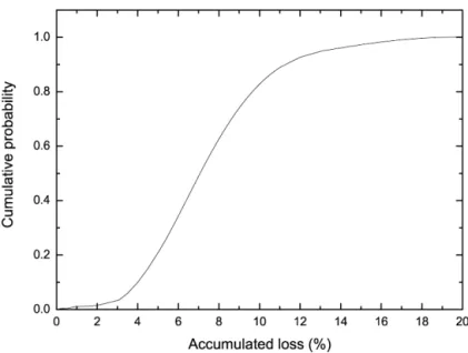
Now we give a numerical example to get the loss distribution ofL

(

t

)

by using the fast Fourier transform. For convenience, we assume Ai

=

A

=

0

.

4 fori

=

1

,

2

, . . . ,

n, and letn

=

100,

α

=

1

.

2,

β

= −

0

.

5,

γ

=

0

.

5,q

=

0

.

3; p

=

0

.

2,

ρ

1

=

0

.

1,

ρ

2

=

0

.

2, l

=

0

.

80. We illustrate the cumulative probability of accumulated loss in Fig. 1.

4.2. Case for symmetric dependence structure

Another case for modelling stochastic correlation, takes a more sophisticated way to consider the systemic risk, i.e., the correlation random variable is assumed to follow a symmetric dependence structure

(6)

ρ

i

=

(

1

−

Bs

)(

1

−

Bi

)

ρ

+

Bs

,

i

=

1

, . . . ,

n

,

(27)

where Bs

,

Bi,i

=

1

, . . . ,

n, are independent Bernoulli random variables and constant

ρ

∈ [

0

,

1

]

. We still adopt the expression

in (19) for random variable Bi, and denoteBs as follows:

Bs

=

1

,

with probabilityq

ˆ

,

0

,

with probability 1

− ˆ

q

.

(28)

The general model of (17) can be written as:

Vi

=

(

1

−

Bs

)(

1

−

Bi

)

ρ

+

Bs Y

+

(

1

−

Bs

)

1

−

ρ

2

₍

₁

₋

_B i

)

+

Bi

i

,

i

=

1

, . . . ,

n

,

(29)

then, conditioning onY andBs, we have

pi|Y,Bs=1 t

=

P

(

τ

i

t

|

Y

=

y

,

Bs

=

1

)

=

1_{yAi}

,

(30) pi|Y,Bs=0 t

=

P

(

τ

i

t

|

Y

=

y

,

Bs

=

0

)

=

P

(

1

−

Bi

)

ρ

Y

+

1

−

ρ

2

₍

₁

₋

_B i

)

+

Bi

i

Ai

Y

=

y

,

Bs

=

0

=

P

ρ

Y

+

1

−

ρ

2

i

Ai

Y

=

y

,

Bs

=

0

,

Bi

=

0

P

(

Bi

=

0

)

+

P

(

i

Ai

|

Y

=

y

,

Bs

=

0

,

Bi

=

1

)

P

(

Bi

=

1

)

=

(

1

−

q

)

Ai−ρy

√

1−ρ2

−∞ f_MG-N IG

x

;

0

,

1

;

1

−

ρ

2

ρ

α

,

1

−

ρ

2

ρ

β,

−

1

−

ρ

2

ρ

β

γ

2

α

2

,

1

−

ρ

2

ρ

γ

3

α

2

;

p

dx

+

q Ai

−∞ f_M_G_{-N I}_G

x

;

0

,

1

;

1

−

ρ

2

ρ

α

,

1

−

ρ

2

ρ

β,

−

1

−

ρ

2

ρ

β

γ

2

α

2

,

1

−

ρ

2

ρ

γ

3

α

2

;

p

dx

.

(31)

Now we consider the computation of probability distribution function of the accumulated loss L

(

t

)

. Similar to Section 4.1, we analyze the characteristic function E

[

ejuL(t)

_]

_for_L

₍

_t

₎

_{. Using the tower property to integrate out} _B

s yields E

ejuL(t)

= ˆ

qE

ejuL(t)

Bs

=

1

+

(

1

− ˆ

q

)

E

ejuL(t)

Bs

=

0

,

(32)

where j is deﬁned as in Section 4.1.

Conditioning upon Bs

=

1 (Bs

=

0), next we will give the conditional characteristic functions E

[

ejuL(t)

|

Bs

=

1

]

(E

[

ejuL(t)

|

Bs

=

0

]

, respectively) ofL

(

t

)

as follows:

E

ejuL(t)

Bs

=

1

=

E

ejuL(t)

Y

=

y

,

Bs

=

1

=

∞

−∞ E

eju( n i=1li1{τit})

_Y

=

_y

_,

_B_s

=

₁

_f_M G-N IG

y

;

0

,

1

;

α

, β,

−

β

γ

2

α

2

,

γ

3

α

2

;

p

dy

.

(33)

Since default times are independent conditioning uponY andBs, then

E

eju n i=1li1{τit}

_Y

=

_y

_,

_B_s

=

₁

=

n

i=1 E

ejuli1{τit}

_Y

=

_y

_,

_B_s

=

₁

_,

₍₃₄₎

where the conditional characteristic function of the default loss of theith reference entity can be computed by:

E

ejuli1{τit}

_Y

=

_y

_,

_B_s

=

₁

=

_ejuli_pi|Y,Bs=1 t

+

1

−

pi|Y,Bs=1 t

=

1

+

ejuli

−

₁ _pi|Y,Bs=1 t

.

(35)

Substituting (34) and (35) into (33) yields

E

ejuL(t)

Bs

=

1

=

∞

−∞ n

i=1

1

+

ejuli

−

₁ _pi|Y,Bs=1 t

f_M_G_{-N I}_G

y

;

0

,

1

;

α

, β,

−

β

γ

2

α

2

,

γ

3

α

2

;

p

dy

.

(36)

(7)

E

ejuL(t)

Bs

=

0

=

E

ejuL(t)

Bs

=

0 Y

=

y

=

∞

−∞ E

ejuL(t)

Y

=

y

,

Bs

=

0

f_M_G_{-N I}_G

y

;

0

,

1

;α

, β,

−

β

γ

2

α

2

,

γ

3

α

2

;

p

dy

=

∞

−∞ n

i=1 E

ejuli1{τit}

_Y

₌

_y

_,

_B s

=

0

f_M_G_{-N I}_G

y

;

0

,

1

;

α

, β,

−

β

γ

2

α

2

,

γ

3

α

2

;

p

dy

=

∞

−∞ n

i=1

1

+

ejuli

−

₁ _pi|Y,Bs=0 t

f_M_G_{-N I}_G

y

;

0

,

1

;α

, β,

−

β

γ

2

α

2

,

γ

3

α

2

;

p

dy

.

(37)

Combining (36), (37) with (32), similar to Theorem 4.1, we obtain the following conclusions: Theorem 4.2.The unconditional characteristic function of L

(

t

)

is expressed by

E

ejuL(t)

= ˆ

q ∞

−∞ n

i=1

1

+

ejuli

−

₁ _pi|Y,Bs=1 t

f_MG-N IG

y

;

0

,

1

;

α

, β,

−

β

γ

2

α

2

,

γ

3

α

2

;

p

dy

+

(

1

− ˆ

q

)

∞

−∞ n

i=1

1

+

ejuli

−

₁ _pi|Y,Bs=0 t

f_MG-N IG

y

;

0

,

1

;

α

, β,

−

β

γ

2

α

2

,

γ

3

α

2

;

p

dy

,

(38)

and the loss distribution L

(

t

)

can be derived by the fast Fourier transform. 5. Random factor loadings

As shown by Andersen and Sidenius (see [7]) that the random factor loadings seem to ﬁt market data well. It was therefore a natural extension to see if a combination of the above

M

G-N IG copula model and the random factor loadings

in one model should provide an even better ﬁt. In the following we are going to consider the single factor

M

G-N IG copula

model where the factor loadings depend deterministically on the common factorY.

Following closely the lines of discussion presented by Andersen and Sidenius [7], we express the

M

G-N IG copula model

with random loadings as follows. In this case, theith asset value is modelled by

Vi

=

ρ

i

(

Y

)

Y

+

1

−

Var

ρ

i

(

Y

)

Y

i

+

bi

,

(39) wherebi

= −

E

[ρ

i

(

Y

)

Y

]

.

Now we give a simplest form associated with (39). The factor

ρ

i

(

Y

)

is anR

→

Rfunction to which, following the original

model (see [7]), is given by:

ρ

i

(

Y

)

=

h11{Y<}

+

h21{Y}

,

(40) where

is a positive constant,h1,h2 are some input parameters withh1

,

h2

>

0.

Thus, the conditional default probability givenY of theith asset can be expressed by:

pi_t|Y

=

P

(

τ

i

t

|

Y

=

y

)

=

P

(

Vi

Ai

|

Y

=

y

)

=

1_{y<} Ai

_√

−bi−h1y 1−h2 1

−∞ f_MG-N IG

(

x

;0

,

1;

α

1

, β

1

,

μ

1

,

σ

1

;

p

)

dx

+

1_{y} Ai−bi−

_√

h₂y 1−h2 2

−∞ f_M_G_{-N I}_G

(

x

;

0

,

1

;α

2

, β

2

,

μ

2

,

σ

2

;

p

)

dx

,

i

=

1

, . . . ,

n

,

(41) where bi

= −

h1

−∞ y f_M_G_{-N I}_G

(

y

;

0

,

1

;

α

1

, β

1

,

μ

1

,

σ

1

;

p

)

dy

−

h2 ∞

y f_M_G_{-N I}_G

(

y

;

0

,

1

;

α

2

, β

2

,

μ

2

,

σ

2

;

p

)

dy

,

(42)

α

k

=

1

−

h_k2 hk

α

,

β

k

=

1

−

h2_k hk

β,

μ

k

= −

1

−

h2_k hk

β

γ

2

α

2

,

σ

k

=

1

−

h_k2 hk

γ

3

α

2

,

k

=

1

,

2

.

(43)

(8)

Denote F_M1 G-N IG

Ai

−

bi

−

h1y

1

−

h2₁

=

Ai

_√

−bi−h1y 1−h2 1

−∞ f_M_G_{-N I}_G

(

x

;

0

,

1

;α

1

, β

1

,

μ

1

,

σ

1

;

p

)

dx

,

i

=

1

, . . . ,

n

,

(44) F_M2 G-N IG

Ai

−

bi

−

h2y

1

−

h2₂

=

Ai−bi−

_√

h₂y 1−h2 2

−∞ f_M_G_{-N I}_G

(

x

;

0

,

1

;α

2

, β

2

,

μ

2

,

σ

2

;

p

)

dx

,

i

=

1

, . . . ,

n

,

(45)

then, analogous to the method described in Section 4.1, we arrive at the following results:

Theorem 5.1.The characteristic function E

[

ejuL(t)

_]

_{of the accumulated loss L}

₍

_t

₎

_{of the reference portfolio is given by} E

ejuL(t)

=

−∞ N

i=1

1

+

ejuli

−

₁ _F1 MG-N IG

Ai

−

bi

−

h1y

1

−

h2 1

f_MG-N IG

y

;

0

,

1

;

α

, β,

−

β

γ

2

α

2

,

γ

3

α

2

;

p

dy

+

∞

N

i=1

1

+

ejuli

−

₁ _F2 MG-N IG

Ai

−

bi

−

h2y

1

−

h2 2

f_M_G_-_{N I}_G

y

;

0

,

1

;

α

, β,

−

β

γ

2

α

2

,

γ

3

α

2

;

p

dy

,

(46)

and the distribution of L

(

t

)

can be derived from the fast Fourier transform. Acknowledgments

We thank the referee for his valuable comments, constructive and useful remarks improving the paper. The research is supported by National Science Foundation of China (Grant No. 70771018), Postdoctor Science Foundation of China (Grant No. 20070410350), Social Science Foundation of Ministry of Education in China (Grant No. 05JA630005) and the Project of New Century Excellent Talent of Ministry of Education in China (2005).

References

[1] D.X. Li, On default correlation: A copula approach, J. Fixed Income 9 (2000) 43–54. [2] H. Gifford Fong, The Credit Market Handbook, John Wiley & Sons, Inc., New Jersey, 2006.

[3] J. Hull, A. White, Valuation of a CDO and annth to default CDS without Monte Carlo simulation, J. Derivatives 2 (2004) 8–23. [4] J.-P. Laurent, J. Gregory, Basket default swaps, CDOs and factor copulas, J. Risk 7 (2005) 103–122.

[5] X. Burtschell, J. Gregory, J.-P. Laurent, A comparative analysis of CDO pricing models, Working Paper, ISFA Actuarial School, University of Lyon & BNP-Paribas, online athttp://www.defaultrisk.com, 2005.

[6] L. Schloegl, Modelling correlation skew via mixing copulae and uncertain loss at default, Presentation at the Credit Workshop, Isaac Newton Institute, 2005.

[7] L. Andersen, J. Sidenius, Extensions to the Gaussian copula: Random recovery and random factor loadings, J. Credit Risk 1 (2005) 29–70.

[8] Claudio Ferrarese, A comparative analysis of correlation skew modeling techniques for CDO index tranches, Department of Mathematics, Kings College London, United Kingdom, online athttp://www.defaultrisk.com, 2006.

[9] A. Kalemanova, B. Schmid, R. Werner, The normal inverse Gaussian distribution for synthetic CDO, J. Derivatives 3 (2007) 80–93.

[10] Geng Xu, Extending Gaussian copula with jumps to match correlation smile, Wachovia Securities, online athttp://www.defaultrisk.com, 2006. [11] Dezhong Wang, Svetlozar T. Rachev, Frank J. Fabozzi, Pricing tranches of a CDO and a CDS index: Recent advances and future research, Working Paper,

University of California, Santa Barbara, 2006.

[12] X. Burtschell, J. Gregory, J.-P. Laurent, Beyond the Gaussian copula: Stochastic and local correlation, Working Paper, ISFA Actuarial School, University of Lyon & BNP-Paribas, online athttp://www.defaultrisk.com, 2005.