Scholarship@Western
Scholarship@Western
Electrical and Computer EngineeringPublications Electrical and Computer Engineering Department
2021
A Systematic Review of Convolutional Neural Network-Based
A Systematic Review of Convolutional Neural Network-Based
Structural Condition Assessment Techniques
Structural Condition Assessment Techniques
Sandeep SonyWestern University
Kyle Dunphy
Western University
Ayan Sadhu
Western University, [email protected]
Miriam A M Capretz
Western University, [email protected]
Follow this and additional works at: https://ir.lib.uwo.ca/electricalpub
Part of the Civil and Environmental Engineering Commons, Computer Engineering Commons, and the
Electrical and Computer Engineering Commons Citation of this paper:
Citation of this paper:
Sony, Sandeep; Dunphy, Kyle; Sadhu, Ayan; and Capretz, Miriam A M, "A Systematic Review of
Convolutional Neural Network-Based Structural Condition Assessment Techniques" (2021). Electrical and Computer Engineering Publications. 184.
A Systematic Review of Convolutional Neural
Network-1
Based Structural Condition Assessment Techniques
2
Sandeep Sony
1, Kyle Dunphy
2, Ayan Sadhu
3, and Miriam Capretz
4 31PhD Student, Department of Civil and Environmental Engineering, Western University.
4
2MSc Student, Department of Civil and Environmental Engineering, Western University.
5
3Corresponding Author: Assistant Professor, Department of Civil and Environmental Engineering,
6
Western University, London, Ontario, Canada. Email: [email protected].
7
4Professor, Department of Electrical and Computer Engineering, Western University.
8
Abstract 9
With recent advances in non-contact sensing technology such as cameras, unmanned aerial and
10
ground vehicles, the structural health monitoring (SHM) community has witnessed a prominent
11
growth in deep learning-based condition assessment techniques of structural systems. These deep
12
learning methods rely primarily on convolutional neural networks (CNNs). The CNN networks
13
are trained using a large number of datasets for various types of damage and anomaly detection
14
and post-disaster reconnaissance. The trained networks are then utilized to analyze newer data to
15
detect the type and severity of the damage, enhancing the capabilities of non-contact sensors in
16
developing autonomous SHM systems. In recent years, a broad range of CNN architectures has
17
been developed by researchers to accommodate the extent of lighting and weather conditions, the
18
quality of images, the amount of background and foreground noise, and multiclass damage in the
19
structures. This paper presents a detailed literature review of existing CNN-based techniques in
20
the context of infrastructure monitoring and maintenance. The review is categorized into multiple
21
classes depending on the specific application and development of CNNs applied to data obtained
22
from a wide range of structures. The challenges and limitations of the existing literature are
23
discussed in detail at the end, followed by a brief conclusion on potential future research directions
24
of CNN in structural condition assessment.
25
Keywords: Structural health monitoring, artificial intelligence, deep learning, CNN, damage
26
detection, anomaly detection, structural condition assessment.
27
Sony, S., Dunphy, K., Sadhu, A., & Capretz, M. A systematic review of convolutional neural network-based structural condition assessment techniques. Engineering Structures, 226, 111347.
Table 1. List of acronyms. 28 29 30 31 32 33 34 35 36 37 38 39 40 41 42
1. Introduction
43Structural health monitoring (SHM) offers emerging and powerful diagnostic tools for damage
44
detection, maintenance, life-cycle cost reduction, and rapid disaster management for structures
45
Acronym Description
AdaBoost Adaptive Boosting
AE Auto Encoder
CNN Convolutional Neural Network
DBN Deep Belief Network
DBM Deep Boltzmann Machine
DL Deep Learning
FCN Fully Convolutional Network
kNN k-nearest Neighbor
ML Machine Learning
NN Neural Network
ReLU Rectified Linear Unit
ResNet Residual Network
R-CNN Regional Convolutional Neural Network
RNN Recurrent Neural Networks
ROC Receiver Operating Characteristic
SHM Structural Health Monitoring
SVM Support Vector Machine
TL Transfer Learning
(Cawley 2018). Most of these techniques rely on dynamic measurements that require installation
46
of contact sensors such as accelerometers, strain gauges, fiber optic sensors, and ultrasonic wave
47
sensors, which have high installation costs. With the recent development of next-generation
48
sensors (Sony et al. 2019; Dabous and Feroz 2020) such as digital and high-speed cameras,
49
unmanned ground vehicles (UGVs), and mobile sensors, there has been a radical shift to
non-50
contact sensing techniques in SHM. They are easier to deploy, less labor-intensive, and more
cost-51
effective, enabling more reliable data acquisition from structures with high-resolution temporal
52
and spatial information (Lattanzi and Miller 2017; Almasri et al. 2020). However, unlike
53
traditional contact sensors, non-contact sensors yield images and videos that require significant
54
advances in robotics, image processing, computer vision, and deep learning algorithms, where
55
structural engineers still face several challenges. In recent years, the SHM researchers have
56
explored artificial intelligence techniques to solve these challenges and successfully achieve novel
57
autonomous and intelligent inspection strategies using the non-contact and robotic devices. This
58
research not only accelerates monitoring and maintenance tasks for the infrastructure owners but
59
also allows accurate early-stage defect detection to prevent any catastrophic structural failure in
60
the future. Moreover, the research advancement in this area enables improved structural
61
maintenance with minimal human errors, lower costs, and higher accuracy, providing an
end-to-62
end system to the infrastructure owners. This research has resulted in numerous publications in
63
top-notch structural engineering journals. The main objective of this paper is to provide a
64
systematic review of recent convolutional neural network (a subset of deep learning
methods)-65
based techniques that have been widely developed in the context of non-contact sensing-based
66
SHM.
67
A non-contact sensor such as a camera, where each pixel is effectively a sensor, can remotely
68
collect a large amount of data from a structure. The challenge is then to interpret these images or
69
videos for decision-making in SHM. Since the last decade, the SHM community has seen
70
significant development in various image-processing algorithms that have enhanced the
71
capabilities of non-contact sensors to undertake structural condition assessment. For example,
72
Jahanshahi et al. (2009) reviewed various image processing techniques that were explored for the
73
detection of missing or deformed members, cracks, and corrosion in various structures. A suite of
74
image-based crack acquisition, processing, and interpretation techniques specifically for asphalt
75
pavement was presented by Zakeri et al. (2017). Along similar lines, Koch et al. (2015) presented
a comprehensive summary of various image processing techniques that have been used to identify
77
damage patterns in concrete bridges, tunnels, pipes, and pavement. Recently, Mohan and Poobal
78
(2018) reviewed various image processing techniques for detecting cracks in concrete surfaces and
79
concluded that the direction of the crack was crucial to the ability to detect and quantify the size
80
of cracks.
81
Overall, existing image processing methods extract features from images using various edges or
82
boundary detection techniques such as the fast Haar transform, Canny filter, Sobel edge detector,
83
morphological detectors, template matching, background subtraction, and texture recognition
84
methods. However, these methods often result in ill-posed problems due to disturbances created
85
by environmental conditions such as light, distortion, weather, shade, and occlusion in outdoor
86
civil structures (Lee et al. 2014). The SHM community has recently focused on overcoming these
87
challenges using various computer vision and artificial intelligence (AI) techniques due to their
88
reduced sensitivity to external disturbances and feature selection. Salehi and Burgueno (2018)
89
reviewed a suite of various artificial intelligence (AI) methods that have recently been used in
90
structural engineering. The authors showed the recent trend of AI-assisted research towards pattern
91
recognition and machine learning-based automated data-driven methods. The relative merits and
92
drawbacks of various AI methods were discussed in the context of various structural engineering
93
applications. This paper reviews CNN-based deep learning techniques with a specific focus on the
94
implementationof non-contact sensor-based SHM.
95
Although AI is a broad area of research covering various engineering disciplines, machine learning
96
(ML) and deep learning (DL) techniques are the two most popular branches of AI that have been
97
heavily explored in SHM research. ML algorithms are trained on a wide variety of data, and the
98
accuracy of the algorithms improves with more data. The purpose of training is to optimize the
99
error along the dimensions of the dataset using optimization functions such as a loss function or
100
objective function and to obtain the best prediction results for test data. However, ML algorithms
101
need features that are obtained from different image processing methods and are fed into different
102
classifiers. Depending on the application, a suitable choice of features and classifiers is essential
103
to identify anomalies from the images.
104
Ying et al. (2013) reviewed various ML-based SHM algorithms for isolating structural damage to
105
steel pipes from environmental factors. Recently, another review paper written by Feng and Feng
(2018) provided an intensive literature review of state-of-the-art computer vision techniques using
107
vision-based displacement sensors that were implemented for SHM. Most of these methods were
108
based on template matching algorithms that extracted displacement time-histories from videos and
109
images. The authors discussed various challenges of displacement extraction from videos obtained
110
from 2D and 3D measurements and from artificial or natural targets, as well as their real-time and
111
preprocessing applications. In particular, Gomes et al. (2018) presented a comprehensive review
112
of intelligent computational tools available for damage detection and system identification, with a
113
specific emphasis on composite structures. More recently, state-of-the-art vision-based structural
114
condition assessment techniques using computer vision and ML algorithms were reviewed by
115
Spencer et al. (2019). The challenges associated with static and dynamic measurement techniques
116
were discussed, along with future directions of automated and improved decision-making methods
117
for SHM. Overall, it can be concluded from the literature that ML methods rely heavily on feature
118
extraction, followed by the application of suitable classifiers. These methods can manage small
119
anomaly datasets, but may not be adequate for full-scale civil structures such as buildings, bridges,
120
dams, pipelines, and wind turbines where crack patterns are complex and irregular (Yao et al.
121
2014).
122
Unlike ML, DL-based AI methods automatically extract features and eliminate the need for
123
manual feature extraction. Therefore, DL can differentiate among a large number of classes, and
124
this capability has been recently explored for damage evaluation in structures. DL algorithms are
125
based on vast sets of labeled data and require high computational performance and memory
126
requirements. The term “deep” refers to the large number of layers that exist between the raw
127
image input and the final classification output used in a network. Convolutional neural networks
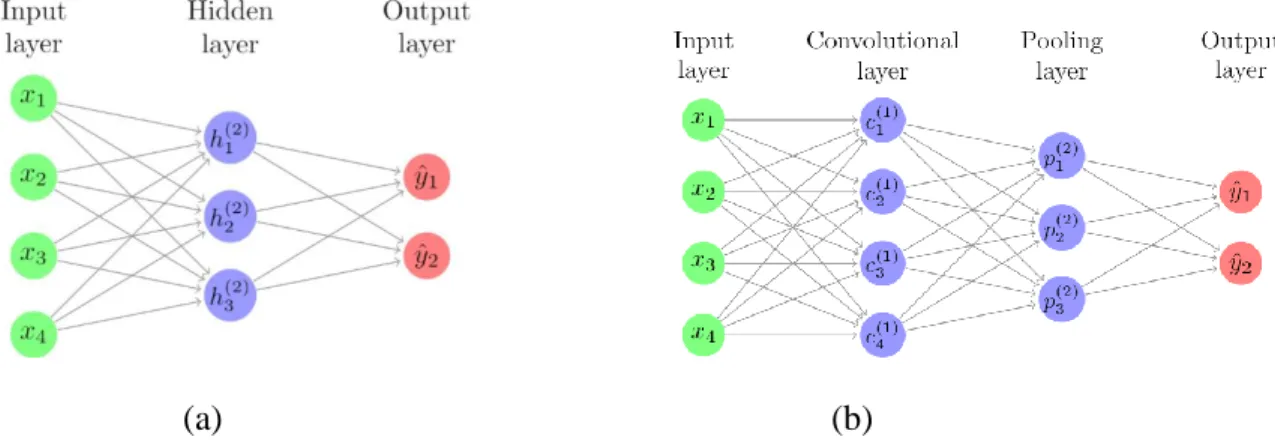
128
(CNNs), which are a popular class of DL methods, have been successfully used since their
129
breakthrough in the 2012 ImageNet challenge due to their ability to extract features automatically.
130
This has enabled automatic and optimized feature extraction to become part of the classifier
131
learning process, which, however, does not compromise its optimality or the accuracy of crack
132
identification. In particular, Bao et al. (2019) briefly reviewed improved SHM techniques that
133
explored various data science, computer vision, DL, and ML methods. It was concluded that the
134
application of DL, ML, and computer vision techniques made it possible to extract pertinent data
135
from noisy measurement databases with damage signatures and to analyze them without requiring
136
any predefined classifiers. Zhao et al. (2015) and Lei et al. (2020) summarized various ML and
DL techniques and their applications that are specific to machine health monitoring. It was
138
concluded that DL techniques were the most effective because they are not restricted to specific
139
machine types and involve minimal human intervention. Recently, Ye et al. (2019) provided a
140
general survey and overview of various DL techniques in the context of SHM. Considering the
141
intensity of CNN-based literature in the field of infrastructure monitoring, this paper is intended
142
to provide a systematic review of standalone CNN-based literature that is specific to structural
143
condition assessment.
144
The key objectives of this review paper are as follows:
145
1. To review CNN-specific papers that have been recently explored for structural condition
146
assessment, with a specific focus on structural damage and anomaly detection. Similar to
147
the condition monitoring of machines, there has been a significant trend towards using
148
CNN to undertake local damage assessment and anomaly detection in large-scale civil
149
structures. The primary objective of this paper is to conduct a detailed survey of emerging
150
CNN-based SHM papers and to provide a comprehensive review of more than one hundred
151
papers that have been recently published on this topic.
152
2. To compare existing CNN-based solutions and best practices to address the challenges of
153
infrastructure monitoring and maintenance, which would provide valuable opportunities
154
and guidance to future engineers and researchers to adopt the most relevant CNN
155
architecture depending on their applications.
156
3. To provide a perspective on CNN-based methods in the domain of SHM that would
157
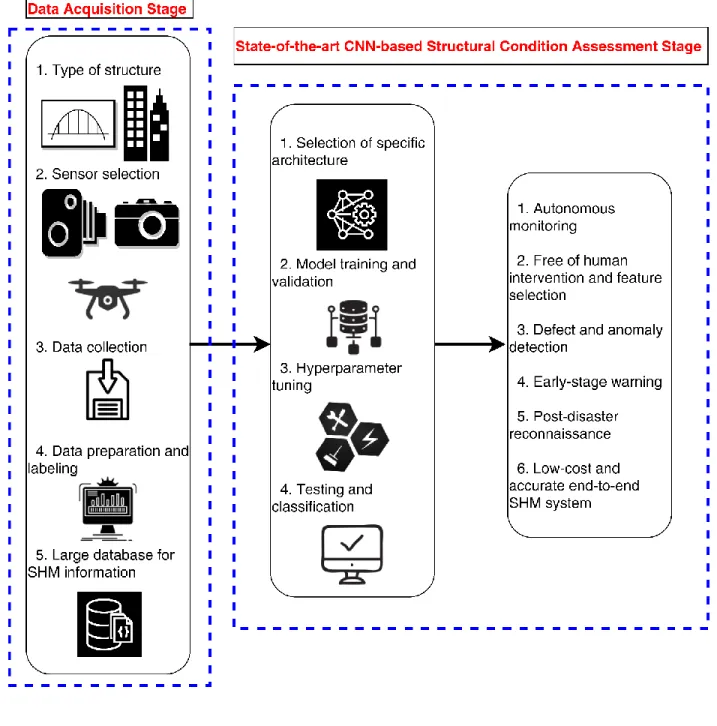
facilitate valuable feature selection and anomaly detection methodologies in other areas of
158
structural engineering and the broader field of civil engineering.
159
4. To provide the key challenges of the current literature and identify the potential future
160
research directions of the CNN-based research in structural condition assessment.
161
This paper is structured as follows. A brief overview of various DL methods and CNN techniques
162
is presented first. Next, the details of various CNN-based condition assessment techniques and
163
their recent applications in structural condition assessment are presented. Different hybrid methods
164
based on CNN are then presented, followed by key conclusions and discussions.
165 166 167
2. Preliminaries of Deep Learning Methods
168Non-contact sensing techniques (Sony et al. 2019; Dabous and Feroz 2020) and computer vision
169
(Feng and Feng 2018; Spencer et al. 2019; Dick et al. 2019) have opened up a new era of
next-170
generation autonomous SHM and inspection of large-scale structures. These sensors result in
171
images and videos, requiring AI techniques to analyze complex input-output relationships of the
172
training data and develop predictive models. The trained predictive models are then used for
173
damage classification, localization, and prediction from the new measurement data of a wide range
174
of structures. The objective of this paper is to review CNN-based SHM papers that have been
175
published in the specific context of structural condition assessment. A brief background on DL
176
methods is presented next, followed by a detailed background on CNN techniques.
177
DL algorithms have an adaptable nature similar to the human brain. These algorithms become
178
more accurate as more training data are provided to them. DL models can simultaneously learn
179
representation and decision rules from the data, like the biological organisms by which they are
180
inspired. DL methods have multiple layers of non-linear transformations. For example, a raw
181
image dataset that is fed through any DL architecture passes through several layers. Each layer,
182
starting with the input layer, improves the identification of the dataset with subsequent layers, and
183
eventually produces a classification or identification at the output layer (Lee et al. 2018). The most
184
prominent aspect of DL is that these layers are not designed by engineers, but rather are learned
185
from the data using a general-purpose learning procedure (LeCun et al. 2015). The advantage of
186
DL is that it requires minimal user intervention, which has attracted various interdisciplinary
187
researchers to use it for a wide range of applications such as object detection, classification, and
188
segmentation.
189
In the context of SHM, DL can be used for damage detection in three ways: (a) classification, i.e.,
190
labeling an image as damaged or undamaged, (b) localization, i.e., locating the regions where
191
damage exists using bounding boxes and identifying their coordinates, (c) segmentation, i.e.,
192
segmenting the pixels of an image into damaged and undamaged pixels (e.g., labeling of all pixels).
193
In the last few years, several methods have been developed, including, but not limited to, the audio
194
signal, time-series, video, and natural language datasets. DL methods (Goodfellow et al. 2016)
195
have several variants such as Auto Encoders (AEs), Deep Belief Networks (DBNs), Deep
Boltzmann Machines (DBMs), Recurrent Neural Networks (RNNs), and Convolutional Neural
197
Networks (CNNs).
198
The AE algorithm is used to learn data coding in an unsupervised manner to create a representation
199
for a dataset by dimensionality reduction, ignoring the noise in the dataset (Vincent et al. 2008).
200
DBN is a probabilistic generative model composed of multiple layers of stochastic and latent
201
variables. If the number of units in the highest layer is small, DBN performs
non-202
linear dimensionality reduction and can learn short binary codes that enable very fast retrieval of
203
datasets (Hinton et al. 2006). DBM is a type of binary pairwise Markov random field with multiple
204
layers of hidden random variables. Similarly to DBN, DBM can learn a complex and abstract
205
internal representation of the input dataset using a limited amount of labeled data (Salakhutdinov
206
and Hinton 2009). RNNs are designed and tested for sequential data, typically for application in
207
dynamic systems such as time-series or speech and language. RNNs are the deepest of all neural
208
networks and can generate memories of arbitrary sequences of input patterns (Funahashi and
209
Nakamura 1993). However, CNNs require less statistical and probabilistic expertise to run and to
210
infer the dataset and results, which makes them a preferred choice for researchers in the SHM
211
community. The next section presents a detailed background on CNN, followed by a systematic
212
literature review of non-contact sensor-based SHM using CNN.
213
3. Background on Convolutional Neural Networks
214CNN is the most popular variant of the DL network. The underlying architecture of CNN is
215
comprised of three layers: (a) convolutional (feature extraction), (b) pooling (dimensionality
216
reduction), and (c) fully-connected layer. The convolutional layer contains a finite number of
217
filters (defined by the kernel or filter size) that convolves with the input data and identify a large
218
number of relevant features from the input image. The pooling layer reduces the dimensions of the
219
resulting features using a down-sampling operation, thereby minimizing the overall computational
220
effort of the network. Depending on the data and the desired accuracy, the system is deepened by
221
repeating the convolution-pooling sequences multiple times. In this way, more high dimensional
222
features are extracted from the input data followed by one or several fully-connected layers that
223
are used for classification. Various C++/Python-based frameworks and platforms (Pouyanfar et al.
224
2018), including TensorFlow, PyTorch, Caffe, Theano, and Keras, are currently available to
225
execute these tasks.
Combined with advances in GPUs and parallel computing, CNNs are a key technology underlying
227
new developments in automated driving and facial recognition. CNNs are trained using a
228
backpropagation algorithm, which combines the chain rule with the principles of dynamic
229
programming. In a traditional neural network (NN), the full connections between the layers lead
230
to time-intensive computations and overfitting of parameters (Abiodun et al. 2018). Unlike NN, a
231
CNN convolves by using particular layers and avoids general multiplications, thereby keeping
232
computations faster. CNN passes the input images through many deep layers (Gu et al. 2017; Yao
233
et al. 2019) such as convolutional, pooling, and activation layers for feature extraction and
234
performs classification using fully connected layers with a non-linear classifier (e.g., a Softmax
235
classifier). CNN attempts to extract features by alternating and stacking convolutional kernels and
236
pooling tasks. It tries to find features that best describe the input images with a varying number of
237
deep layers. A rectified linear unit (ReLU) is often used as a non-linear activation function to
238
introduce non-linearity in one or more of these layers on CNN. Auxiliary layers such as dropout
239
layers are also used to prevent overfitting on CNN.
240
Convolutional layers take an input image and convolve it with a filter or kernel, where the size of
241
the kernel matrix is much smaller than the size of the input matrix. The matrix multiplication of
242
convolutional layers reduces the number of weights, which reduces the variance of the model.
243
Convolutions generate invariant local features; at a lower level, filters can be used to detect edges
244
in the image, whereas at a higher level, they can detect more complex shapes and objects that are
245
critical for classifying an image. A convolutional layer is a set of image filters with learnable
246
weights and plays an important role in CNN as a feature extractor.
247
On the other hand, pooling layersreduce the size of the layer while reducing the number of neurons
248
in networks and extracting the most significant features with fixed-length over sliding windows of
249
the raw input data. The reduction in the number of neurons is carried out by sliding a fixed window
250
across a layer and choosing one value that effectively represents all the units captured by the
251
window. Max-pooling and average-pooling are two common implementations of pooling. In
max-252
pooling, the representative value becomes the largest of all units in the window, whereas, in
253
average-pooling, the representative value becomes the average of all units in the window. A
max-254
pooling layer is mostly used to down-sample the filtered weights from the convolutional layer,
255
reducing computational costs and the probability of overfitting.
A fully connected layer has the shape of a flattened vector and plays an active role as a connector
257
between the two-dimensional convolutional layer and the one-dimensional Softmax layer. The
258
Softmax layer takes features from the fully connected layer, calculates the probabilities of each
259
class using a normalized exponential function, and outputs the class with the highest probability
260
as the classification result. By passing the images through various layers, a large number of
261
parameters at various layers are optimally tuned and can extract salient features from the training
262
images. In general, the training process varies from a few hours to a couple of days, depending on
263
the network and hardware configurations, the training images, and the learning rate.
264
Both ordinary NNs and CNNs are feedforward neural networks and are generally trained using
265
backpropagation. The primary difference between NNs and CNNs is the difference in the layers
266
they use to classify images. Figure 1 shows the schematics of a typical NN and CNN architecture.
267
The NN uses hidden layers (denoted as h), whereas CNN uses convolutional (denoted as c) and
268
pooling layers (denoted as p) along with input and output layers. The number of layers depends on
269
the architecture, the data, and the performance required from the model. One of the most critical
270
issues with NNs is overfitting. Large neural nets trained on relatively small datasets can over-fit
271
the training data. Unlike NNs, CNNs are not prone to overfitting due to a reduction in weights and
272
the number of neurons caused by the convolutional layer and pooling layer, respectively. The
273
difference between NN and CNN can be understood using an example of an image. Consider an
274
image of W * H * 3 (over three channels, red, blue, and green), where W and H denote the width
275
and height of the image matrix, respectively. An ordinary NN will take the image as the input, pass
276
it through fully connected layers and non-linearities, and finally output a vector of probabilities
277
for each class. The fully connected layer is so named because each of the input neurons ni is
278
connected to each output neuron no. If the number of input neurons is assumed to equal to the
279
number of output neurons, the resulting number of weights becomes considerably large (ni * no).
280
In the framework of image classification, it is computationally expensive to train such a network,
281
and it also gives rise to high variance. CNNs are a neural network with a different architecture that
282
significantly reduces the number of weights and, thereby, the variance of the model.
284
(a) (b)
285
Figure 1. Schematic of (a) a typical NN and (b) a typical CNN with convolutional and pooling
286
layers.
287
3.1 CNN Architectures
288LeNet (LeCun et al. 1998) was originally developed to classify low-resolution images such as
289
handwritten alphanumeric characters. AlexNet (Krizhevsky et al. 2012), a popular ImageNet CNN
290
model, was developed by researchers from the University of Toronto and used convolutional filters
291
of varying sizes, where the first layer had 11*11 convolution filters. The authors were the first to
292
use rectified linear units (ReLU). Several layers of convolution and max-pooling were used with
293
around 60 million weights, and the model was trained on 2 GPUs. The Visual Geometry Group,
294
VGGNet (Simonyan and Zisserman 2014), was developed by researchers from Oxford University
295
and only used 3*3 convolutional filters. Conv-Conv-Conv-pool layers were stacked together,
296
followed by fully connected layers at the end. This research showed how the depth of CNN
297
influences the accuracy of image reconstruction.
298
GoogleNet (Szegedy et al. 2014) was a deeper network, containing 22 layers with more
299
computational efficiency, and did not have any fully connected layers. There were around 5 million
300
parameters in the model. The network was composed of stacked sub-networks called inception
301
modules. It had a naïve inception module that ran convolutional layers in parallel and concatenated
302
the filters together. Moreover, it had a dimensionality reduction inception module that performed
303
1*1 convolutions, thereby achieving dimensionality reduction. The reduction lowered the
304
computational cost and made the network computationally efficient by stacking multiple inception
305
modules together. ResNet (He et al. 2015) was deeper than GoogleNet with 152 layers, where each
306
layer in the residual block was implemented as a 3*3 convolution.
The development of newer CNN architectures evidenced a trend towards using more and more
308
layers (i.e., a deeper architecture). Using these architectures for structural damage classification is
309
valid only if a large amount of damage data is available. Moreover,the issue of overfitting may
310
arise, and the outcome of high-performing CNNs will not generalize the results for civil
311
engineering applications.
312
4. Review of CNN-Based SHM Literature
313Primarily originated for object recognition, 2D CNN algorithms were mostly explored for 2D
314
images in various SHM applications to detect defects and anomalies autonomously. Moreover, for
315
vibration-based SHM, the researchers attempted to reshape the vibration signal into images by
316
transforming the signal in frequency and time-frequency (TF) domain and used the resulting TF
317
maps as the images in 2D CNN. However, the images involve significant complexity in choosing
318
a large number of labeled data and layers and are not suitable for real-time SHM applications using
319
mobile or handheld devices. To alleviate this problem, 1D CNN was recently introduced such that
320
a time-history of vibration signal can be directly fed into CNN, which requires simple array
321
operations, thereby demanding a shallow architecture with a fewer number of hidden layers
322
(Kiranyaz et al. 2019).
323
Figure 2 shows a flowchart of the state-of-the-art CNN-based SHM literature that leads to
324
significant advancement in this topic in the last few years. The schematic presents the two stages:
325
data acquisition and condition assessment stage. The data acquisition stage is central to understand
326
which type of data is apt for a particular structure. The data preparation precedes the data
327
acquisition stage, depending on the classification or prediction task required from a specific
328
application. Specific CNN architecture is selected next, followed by their further improvement
329
using hyperparameter tuning. Once this step is accomplished, various infrastructure monitoring
330
tasks are achieved in the last stage, demonstrating the novel contributions of the state-of-the-art
331
CNN-based SHM techniques. A detailed systematic review of CNN-based SHM is organized by
332
classifying the current literature into multiple classes, as illustrated below.
333 334
335
Figure 2. A schematic of the state-of-the-art CNN-based SHM operations.
336
4.1 Bridge health monitoring
337The bridge infrastructure is critical for transportation and requires continuous monitoring. The
338
critical components of any bridge that are prone to damage are used to acquire data in the form of
339
an acceleration time-history, images, or continuous video streams. Deep learning methods such as
340
CNN, FCN, or R-CNN are used to identify, classify, and quantify the damage. Guo et al. (2014)
341
explored a sparse coding-based CNN algorithm with wireless sensors for efficient bridge SHM.
Sparse coding was used as an unsupervised layer for unlabelled data to learn high-level features
343
from acceleration data. Various levels of damage cases were considered for a three-span bridge
344
that was instrumented using wireless sensors. The proposed method was compared with other
345
methods such as logistic regression and decision trees, and the proposed method was shown to
346
outperform other methods with an accuracy of 98%. Gulgec et al. (2017) proposed a methodology
347
for structural damage identification using CNN. Numerous undamaged and single-damaged
348
samples of a steel gusset plate connection created in ABAQUS with varying uniformly distributed
349
loads were developed to train, validate, and test the algorithm. Moreover, 50 network
350
configurations with various hyper-parameters were tested over several epochs to determine the
351
optimal CNN parameters.
352
A multiscale CNN was developed by Narazaki et al. (2017) to extract damage to various bridge
353
components from image-based data. Post-processing methodologies such as super-pixel averaging
354
and conditional random field optimization were implemented to enhance the accuracy of the
355
multiscale CNN. The proposed CNN network was developed from a ResNet made up of 22 layers
356
that computed the Softmax probabilities corresponding to ten scene components. The pixel-wise
357
accuracy was calculated to be only 78.94% for this methodology, suggesting a strong dependence
358
on the quality of super-pixel segmentation with regards to the boundary segmentation of
359
components. An ensemble framework combining a couple of sparse coding algorithms and a CNN
360
was proposed by Fallahian et al. (2018) for structural damage assessment under varying
361
temperature effects. Features extracted from the frequency response function of the measured data
362
were fed into a CNN and a couple of sparse coding algorithms to develop the classifier. Stochastic
363
gradient descent was used in CNN to assign weights, and a Softmax function as an activation
364
function. The proposed method was validated using a numerical truss bridge and a full-scale
365
bridge. However, there are various types of bridges, and for continuous and autonomous
366
monitoring, the identification of various bridge types is critical along with that of multiple damage
367
types.
368
Zhao et al. (2018) explored CNN for maintenance and inspection of bridges. For bridge
369
classification, an AlexNet-based CNN was trained first with more than 3800 images of various
370
bridges. For recognition of bridge components, a ZF-Net-based faster R-CNN was trained with
371
600 bridge images. To detect cracks, a GoogleNet-based CNN was trained with 60000 cracked
372
and un-cracked images. Accuracies of 96.6% for bridge classification, 90.45% for bridge
component classification, and 99.36% for crack detection during testing were achieved. An
image-374
based approach was proposed by Liang (2018) for holistic post-disaster inspection of reinforced
375
concrete bridges using a DL encompassing system level, a component level, and local damage
376
detection. Algorithmically, the network was made up of a VGG-16 TL-based NN with Bayesian
377
optimization for classification, a faster R-CNN for component detection, and a fully deep CNN for
378
semantic damage segmentation. In a similar order, Kim et al. (2018) explored the application of
379
regions with CNN (R-CNN)-based TL to identify cracks in a concrete bridge that were monitored
380
using a UAV. Data containing 50000 images of 32×32 pixels from ImageNet and Cifar-10 were
381
used to train and classify the data. Max pooling and ReLU layers were used along with the
382
convolutional layer in a sliding window-based CNN. The total length and thickness of cracks were
383
also computed using a planar marker and automatically visualized on the inspection map.
384
Bao et al. (2019) presented computer-vision and DL-based structural anomaly detection to achieve
385
automated SHM. Stacked AE and greedy layer-wise training techniques were used to train the DL
386
networks. The acceleration data from a long-span bridge were first converted into images that were
387
then transformed into grayscale image vectors for training a DNN considering six different
388
anomalies such as missing, minor, outlier, square, drift, and trend data points. Recently, Xu et al.
389
(2019) proposed fusion CNN for multilevel and multiscale damage identification in steel box
390
girders without any prior assumptions of crack geometry. The proposed CNN architecture
391
consisted of several layers of convolution, batch normalization, ReLU, max pooling, and Softmax,
392
and was implemented using MatConvNet. Each image containing one or more cracks, handwriting,
393
and background noise was acquired using a consumer-grade camera that was used for training and
394
validation. The authors showed that fusion CNN worked better than general CNN, with an
395
accuracy of 96.38%. However, its performance was limited to a specific object distance and the
396
focal length of the camera.
397
Recently, Ni et al. (2019) proposed a 1D CNN-based technique in combination with autoencoder
398
data compression for anomaly detection in a long-span suspension bridge. An accuracy of 97.53%
399
was achieved with a compression ratio of 0.1. Similarly, Azmi and Pekcan (2019) proposed a
400
CNN-TL-based SHM technique for damage identification in highly compressed data. A four-story
401
numerical quarter-scale IASC-ASCE SHM model was used for numerical verification, and the
402
proposed model was also validated on experimental studies using the IASC-ASCE SHM
403
benchmark building and the Qatar University Grandstand Simulator. A mean accuracy of 90-100%
was achieved using the proposed model. 1D CNN was also used in a further study by Zhang et al.
405
(2019) to detect changes in stiffness and mass. Three structural assemblages, a T-shaped steel
406
beam, a short steel girder bridge, and a long steel girder bridge, were used, and accuracies of
407
99.79%, 99.36%, and 97.23% were achieved.
408
4.2 Pavement condition monitoring
409Pavements are highly susceptible to damage due to high traffic and extreme weather conditions.
410
The dataset usually consists of images acquired from a dashboard camera or a UAV. Cha et al.
411
(2017) introduced a vision-based methodology for detecting cracks in concrete structures using
412
CNN. Using nearly 40,000 images of damaged and undamaged concrete generated from various
413
structures, CNN was tested and validated with more than 97% accuracy. Zhang et al. (2017)
414
proposed a pixel-level CNN to detect cracks on 3D pavement surfaces. The proposed CNN,
415
“CrackNet”, was made up of two fully connected layers, one convolutional layer, one 1 * 1
416
convolution layer, and one output layer. This network was more efficient than traditional CNNs
417
because of the absence of pooling layers that downsized the output of previous layers. An
418
automated crack-length detection algorithm was proposed for pavement by Tong et al. (2017)
419
using a deep CNN. A database of 8000 images of cracked and non-cracked pavement was
420
generated for training, 500 of which were randomly selected to act as the test database. In addition,
421
the images were converted to a grey-scale .bmp format so that k-means clustering analysis could
422
be used to extract the length and shape of each pavement crack accurately. A five-layer-deep CNN
423
achieved an accuracy of 94.35% with a mean squared error of 0.2377 cm for crack lengths between
424
0 and 8 cm. In addition, it was concluded that image resolution and lighting conditions had minimal
425
influence on the accuracy of the proposed crack detection method.
426
Another pavement crack detection approach was investigated by Gopalakrishnan et al. (2017,
427
2018) using TL-based deep CNN. By implementing a truncated VGG-16 deep CNN pre-trained
428
on the ImageNet database, image vectors were extracted to train various classifiers to compare
429
their performance for crack detection. Fan et al. (2018) proposed CNN to detect pavement cracks
430
from images acquired by an iPhone from pavements in Beijing, China. Millions of monochromatic
431
and RGB image patches were used. It was demonstrated that the proposed methodology had a
432
precision of approximately 92%, which was better than traditional ML techniques such as local
433
thresholding, CrackForest, Canny, minimal path selection, and free-form anisotropy. Similarly,
Maeda et al. (2018a,b) investigated the capabilities of CNN networks to detect road surface
435
damage from smartphone images. A pavement image dataset of 9,053 images captured using a
436
dashboard-mounted smartphone was annotated using 15,435 bounding boxes to distinguish
437
various damage classes. By analyzing this dataset using two object detection methods, Single-Shot
438
Multibox Detector (SSD) using Inception V2 and SSD using MobileNet, the robustness of these
439
algorithms was investigated. Although the recall value of longitudinal construction joints and
440
rutting, bumps, potholes, and separation was relatively low due to the small size of the training
441
dataset, SSD MobileNet detected all damage classes with greater than 75% accuracy.
442
Fan et al. (2019) developed a novel FCN with an adaptive thresholding technique for image-based
443
detection of road cracks. Initially, the FCN classified the images as either positive or negative
444
based on the presence of cracks. The positive images were segmented, and an adaptive threshold
445
technique that minimized the within-cluster sum of squares was used to localize the defects. The
446
study used 40,000 RGB images from training, validation, and testing. The proposed methodology
447
exhibited a precision of 99.92% and 98.70% for classification and pixel-level determination of
448
pavement cracks. In another study, Zhang et al. (2018) proposed a novel algorithm to classify
449
sealed and unsealed cracks in asphalt pavement using a TL-based deep CNN. The proposed
450
methodology consisted of three components: (a) the images were initially enhanced to eliminate
451
imbalance from illumination, (b) the images were classified as cracks, sealed cracks, or
452
background images by means of a TL-based DCNN, and (c) fast block-wise segmentation and
453
tensor voting curve detection were used to locate and extract those pixels that were considered
454
cracked or sealed. It was concluded that the proposed method showed superior performance in
455
both the classification and detection of sealed and unsealed pavement cracks. 456
Another DL algorithm was developed through TL for automated crack detection on concrete
457
surfaces (Kim and Cho (2018)). Initially, a database of 50,000 images was created using the
458
commercial scraper, “ScrapeBox”,and various data augmentation techniques. By means of TL, a
459
modified network for multiple object detection, “AlexNet”, was used to train the proposed CNN
460
classifier to identify uncracked pavement, cracks, and single or multiple edges or joints. By
461
defining “crack-like” classes such as edges and joints, the number of false positives was
462
significantly reduced.
463 464
4.3 Inspection of underground structures
465Underground structures such as sewer pipes and tunnels are inaccessible for inspection. The
466
underground structures are monitored using videos in combination with deep learning techniques.
467
Stentoumis et al. (2016) presented CNN-based vision techniques to reconstruct 3D cracks with the
468
aid of a stereo matching and optimization scheme using data acquired from a tunnel by a DSLR
469
camera. A multilevel perceptron CNN was used as a classifier. The proposed method was also
470
compared with various ML techniques such as kNN and SVM. The proposed CNN was shown to
471
outperform other methods, with an accuracy of 88.6%. Similarly, Cheng and Wang (2018)
472
evaluated sewer pipe defects through images acquired from closed-circuit television using faster
473
region-based CNN (faster R-CNN). The R-CNN architecture works based on a region proposal
474
network that can generate region proposals with different aspect ratios and scales to differentiate
475
foreground and background noise to localize an anomaly compared to the undamaged section of a
476
region of 3000 images. Doulamis et al. (2018) proposed a combined CNN and fuzzy spectral
477
clustering approach for real-time crack detection in tunnels. An autonomous robotic system
478
consisting of a robotic vehicle and a robot arm was used to capture imagery along the tunnel. To
479
analyze complex concrete tunnel images, CNN was first used to capture specific regions of
480
damage, followed by fuzzy clustering to exploit the spatial and orientation coherence of the cracks.
481
It was concluded that the accuracy of crack prediction was relatively low due to limited visibility
482
in the tunnel.
483
The capabilities of region-based FCN were explored by Xue and Li (2018) for shield tunnel lining
484
defects. The proposed FCN consisted of a backbone convolutional layer and a pooling layer along
485
with a Softmax layer and bounding box regression. A dataset containing a total of 4139 images of
486
3000×3724 pixels each were acquired using a movable tunnel inspection system consisting of
487
several CCD cameras and LEDs as a source of light. The proposed method outperformed AlexNet
488
and GoogleNet and achieved an accuracy of 96% while performing both object detection and
489
image classification. Recently, Feng et al. (2019) developed a TL based on the Inception-v3 DL
490
algorithm to perform multiple damage type classification for hydro-junction infrastructure. The
491
existing structure of the Inception-v3 algorithm was modified so that the final layer had five fully
492
connected neurons to increase the accuracy of labeling each damage type. In another study (Kang
493
et al. 2020), a basic pursuit-based background filtering algorithm was proposed to improve the
visibility of underground objects (e.g., cavities, manholes, and pipes), followed by DCNN using
495
three-dimensional ground-penetrating radar data from urban roads in Korea.
496
4.4 Building condition assessment
497Tall buildings and historical structures pose a challenge for manual inspection and require an
498
accessible way for autonomous monitoring. Chaiyasarn et al. (2018) proposed an integrated
499
algorithm combining CNN with classification models such as SVM and random forest for crack
500
detection in historic structures. The data consisted of images from masonry structures containing
501
cracks that were acquired using a digital camera and an unmanned aerial vehicle (UAV). It was
502
shown that CNN with SVM outperformed conventional CNN based on the Softmax classifier.
503
Similarly, Yuem et al. (2018) used CNN for image classification after post-event (e.g., earthquake,
504
hurricane, tornado, or others) building reconnaissance. The dataset of 90000 colored structural
505
images was used to train the network for scene classification and object detection. All the images
506
were manually labeled using in-house annotation software before the CNN training phase.
507
To classify various common types of building damage, Perez et al. (2019) explored the possibility
508
of detecting common building defects caused by dampness, such as mold, deterioration, and
509
staining through images using CNN. The proposed model was trained using the VGG-16 (
ResNet-510
50) CNN classifier, and class activation mapping was used for object localization. The CNN
511
architecture contained five blocks of convolutional layers with max-pooling for feature extraction.
512
The proposed methodology achieved an overall accuracy of 87.50% and classified multiclass
513
defects using a small dataset. Recently, Jiang and Zhang (2019) used a wall-climbing unmanned
514
aerial system (UAS) to acquire real-time video. The video data were then converted to 1330 crack
515
images, and a CNN was trained. The images were transferred to an Android platform through a
516
wireless data link. An accuracy of 94.48% was achieved using the proposed model.
517
4.5 Multi-class structural monitoring
518Structures experience multiple types of damage, and identifying all of them at once is a faster
519
approach to repair and maintenance. A vision-based multiscale pixel-wise deep CNN network was
520
proposed by Hoskere et al. (2017) to detect six types of structural damage. The proposed
521
methodology consisted of two parallel steps: (a) a damage classifier to separate each pixel into
522
predefined classes and (b) a damage segmenter that distinguished damaged pixels from undamaged
ones. By implementing 1695 images of over 250 structures, the authors concluded that ResNet23
524
and VGG-19 were the most accurate segmenter and classifier, with accuracies of 88.8% and 71.4%,
525
respectively. Moreover, by combining the segmenter and classifier networks using Softmax
526
thresholds, the accuracy across all classes was increased from 71.4% to 86.7%. Lin and Nie (2017)
527
used a CNN with batch normalization to extract and localize structural damage in a simply
528
supported Euler-Bernoulli beam. Numerical simulations were conducted with various damage
529
locations and conditions to generate a dataset of 6,885 measurements. The proposed methodology
530
was compared with a wavelet packet transform approach for both noiseless and noisy single- and
531
multi-damage scenarios. Overall, CNN resulted in superior performance over the wavelet packet
532
transform for single and multiple structural damage sites.
533
Atha and Jahanshahi (2018) evaluated corrosion detection using three proposed CNN
534
architectures, VGG-15, Corrosion5, and Corrosion7. A comparison is presented with the other two
535
state-of-the-art CNN architectures, VGG-16, and ZF-Net. An approach containing
non-536
overlapping sliding windows was used to isolate the corroded region within each image. The
537
authors investigated the performance of the proposed architecture under various sizes of sliding
538
windows and color spaces. Using two specific properties of CNN (parameter sharing and local
539
connectivity), Khodabandehlou et al. (2018) proposed a CNN method that used a reduced number
540
of parameters, hence requiring limited training data for SHM. Behrouzi and Pantoza (2018) used
541
a DL algorithm to identify damage patterns from tagged images of roadways and railways after
542
large seismic events. The authors claimed that the proposed method correctly identified 92% of
543
the roadway images, where 80% of railways were affected by the earthquake. Cha and Kang (2018)
544
carried out damage identification by means of CNN using ultrasonic beacons by geo-tagging a
545
video stream obtained from a UAV. A deep CNN with a sliding window was used as a DL
546
architecture, with ReLU as an activation function and a Softmax function as a classifier.
547
Similarly, Patterson et al. (2018) used DL techniques for seismic damage image classification and
548
developed a user-friendly graphic user interface wrapper where AlexNet and ResNet were used in
549
the pre-trained DL model. Pan et al. (2018) evaluated the efficacy of DBN using multiple restricted
550
Boltzmann machines for structural condition assessment to enable timely decision-making for
551
maintenance. A 1D CNN was proposed by Abdeljaber et al. (2018) for structural damage detection
552
on an SHM benchmark dataset. Although CNNs are primarily used for 2D signals such as images
553
and videos, the authors used the tanh activation function to learn from 1D raw acceleration data
and proposed an enhanced adaptive CNN to identify global structural damage in structures. Images
555
acquired using smartphones and UAVs are viable and inexpensive options for acquiring damaged
556
data from structures. Li and Zhao (2018) evaluated CNN for crack detection on a real concrete
557
surface using cropped images taken from a smartphone. A CNN with binary outputs of the cracked
558
or uncracked concrete surface was used to train GoogleNet. A total of 60000 images with 256 by
559
256 pixels each were used to classify cracked concrete surfaces with an accuracy of 99.39%. An
560
application called Crack Detector was developed and installed in a smartphone to detect cracks in
561
real-time.
562
Dorafshan et al. (2018a) explored the feasibility of using small off-the-shelf UAVs for inspection
563
of concrete decks and buildings using CNNs. The proposed algorithm was first used to train the
564
model using images acquired from a laboratory-scale bridge deck with a low-resolution camera
565
and achieved an accuracy of 94.7%. The proposed CNN was then used to investigate a building
566
by means of transfer learning (TL) using AlexNet with an accuracy of 97.1%. Moreover, Cha et al.
567
(2018) proposed an improved visual inspection method using a faster region-based CNN. The
568
proposed method provided robust detection of multi-surface damage types such as concrete cracks,
569
medium and high corrosion of steel, bolt corrosion, and steel delamination using a variable
570
bounding box and was shown to be more efficient than the authors’ previous work (Cha et al.
571
2017). Moreover, this technique showed promising results for the autonomous detection of
572
structural defects from quasi-real-time video data. On the other hand, Dorafshan et al. (2018b)
573
provided an excellent database for autonomous detection of cracks ranging from 0.06 to 25 mm
574
using CNN on a concrete surface. Spatial- and frequency-domain edge detection methodologies
575
were compared by the same authors (Dorafshan et al. 2018c) using DCNN to detect cracks in
576
concrete structures. It was concluded that AlexNet could detect smaller cracks (86%) more
577
accurately than Laplacian-of-Gaussian (LoG). Moreover, the authors proposed a hybrid
578
methodology that implemented a CNN to categorize images based on the presence of damage,
579
after which those damaged images were further refined at the pixel level by the LoG edge detection
580
technique.
581
Hoskere et al. (2018) explored FCN with residual network architecture for automated
post-582
earthquake image classification. The FCN was capable of semantic segmentation and classification
583
and was combined with a 3D mesh model of the structure for damage representation in building
584
components. The dataset used to train the FCN included 1000 images of 288 by 288 pixels each
and was acquired from post-disaster reconnaissance surveys using a UAV. An accuracy of 91.1%
586
was achieved for damage type identification along with information of structural and
non-587
structural components. Moreover, Rui et al. (2019) developed a two-stage CNN to detect and
588
classify defects in narrow overlap welds. Time-series signals from eddy current testing of defective
589
welds were initially converted to 2D diagrams using a continuous wavelet transform. Before the
590
initial data transformation, the 2D diagrams were entered into a two-step CNN network that (a)
591
identified the presence of defects using binary classification and (b) upon detecting defects, further
592
classified them into five defect types. Although both single-step and two-step CNNs had similar
593
accuracy of approximately 97%, the faster computational time of the two-step method made it
594
more efficient.
595
Recently, Deng et al. (2019) implemented a faster R-CNN to detect handwritten scripts and cracks
596
in concrete surfaces. A modified 21-layer ZF-Net consisting of three neurons to classify
597
background, cracks, and handwriting was trained using a 20% subset of the authors’ generated
598
database of nearly 5000 sub-images. By investigating the influence of handwriting scripts on crack
599
detection, it was concluded that including handwriting scripts as a unique background class
600
significantly increased the accuracy of classifying cracks in concrete surfaces. Furthermore,
601
comparing the proposed methodology with the DL algorithm, ‘You Only Look Once’ (YoLo) v2,
602
showed superior performance, with significantly reduced percentages of false positives detected.
603
Dung and Duc Anh (2019) proposed an FCN for segmented vision-based detection and density
604
evaluation of surface cracks in concrete structures. TL was applied as the FCN encoder was based
605
on the VGG-16 CNN model because this model showed superior performance to ResNet and
606
Inception. Upon training and validation using 500 images, the FCN was shown to have a max F1
607
score and average precision of approximately 90%.
608
Li et al. (2019) proposed an FCN to detect four concrete damage classes: cracks, spalling,
609
efflorescence, and holes, from an established smartphone-based image database. The development
610
of the FCN algorithm was based on TL of weights and biases provided by DenseNet-121 for feature
611
extraction. The algorithm was trained and validated using 2200 images. Compared to SegNet, the
612
proposed methodology offered better performance in detecting various types of concrete damage.
613
In another recent study, the authors (Mei and Gul 2020) used a depth-first search algorithm as a
614
preprocessing tool to eliminate isolated pixels, followed by multilevel feature fusion and crack
615
detection using images obtained from a smartphone.
4.6 Inspection of other large-scale structures
617Large-scale structures are challengingto monitor, and image-based monitoring techniques provide
618
a powerful tool for effective structural monitoring. CNN was implemented to detect surface defects
619
in rails from photometric stereo images acquired in a dark-field setup by Soukup and Huber-Mork
620
(2014). The setup of various light sources at different oblique angles in the dark-field identified
621
the location of cavities through a scattering of applied light. Comparing traditional model-based
622
approaches to the trained CNN, the authors found a significant reduction in a detection error.
623
Furthermore, regularization methods such as training data augmentation and unsupervised
layer-624
wise pre-training were shown to reduce the probability of overfitting due to the size of the available
625
image dataset. Abdeljaber et al. (2017) proposed a nonparametric 1D CNN to extract structural
626
damage from the time-histories of vibration-based responses. In this method, the acceleration at
627
each sensor location was first divided into several frames, each containing a finite number of
628
samples, and then each frame was normalized and fed into a CNN. The probability of damage was
629
then computed to quantify the severity of damage and isolate the damage location. The proposed
630
methodology showed efficient processing of the measured data compared to existing ML
631
techniques, which required significant pre- and post-processing and feature extraction. A
632
laboratory stadium developed in the Qatar University Grandstand Simulator was used to validate
633
the accuracy of the proposed method.
634
Pan et al. (2018) evaluated the efficacy of DBN using multiple restricted Boltzmann machines for
635
structural health assessment to enable timely decision-making for maintenance. Lin et al. (2018)
636
compared CNN with SVM for damage assessment in a three-story laboratory model and concluded
637
that DL methods had less noise sensitivity than shallow learning methods. Chen and Jahanshahi
638
(2018) proposed a CNN method with a naïve Bayes data fusion scheme to detect tiny cracks on
639
metallic surfaces from video data for nuclear inspection applications. This methodology was
640
distinct from previous CNNs because it collected image data from multiple video frames to
641
improve crack localization while using a naïve Bayes decision process to reduce false negatives.
642
Through testing and training of approximately 300,000 images extracted from video frames, it was
643
concluded that this methodology achieved an accuracy of 98.3%, showing significant
644
improvement compared to state-of-the-art ML algorithms.