No. 2008/07
Asymmetric Multivariate Normal Mixture GARCH
Markus Haas, Stefan Mittnik,
Center for Financial Studies
The
Center for Financial Studies
is a nonprofit research organization, supported by an
association of more than 120 banks, insurance companies, industrial corporations and
public institutions. Established in 1968 and closely affiliated with the University of
Frankfurt, it provides a strong link between the financial community and academia.
The CFS Working Paper Series presents the result of scientific research on selected
topics in the field of money, banking and finance. The authors were either participants
in the Center´s Research Fellow Program or members of one of the Center´s Research
Projects.
If you would like to know more about the
Center for Financial Studies
, please let us
know of your interest.
1 Corresponding Author: Institute of Statistics, University of Munich, D-80799 Munich, Germany; E-mail: [email protected]; Phone: +49 (0) 89 21 80 - 25 70; Fax: +49 (0) 89 21 80 - 50 44.
CFS Working Paper No. 2008/07
Asymmetric Multivariate Normal Mixture GARCH
Markus Haas
1, Stefan Mittnik
2,
and Mark S. Paolella
3January 18, 2008
Abstract:
An asymmetric multivariate generalization of the recently proposed class of normal mixture
GARCH models is developed. Issues of parametrization and estimation are discussed.
Conditions for covariance stationarity and the existence of the fourth moment are derived, and
expressions for the dynamic correlation structure of the process are provided. In an
application to stock market returns, it is shown that the disaggregation of the conditional
(co)variance process generated by the model provides substantial intuition. Moreover, the
model exhibits a strong performance in calculating out–of–sample Value–at–Risk measures.
JEL Classification: C32, C51, G10, G11
Keywords: Conditional Volatility, Finite Normal Mixtures, Multivariate GARCH, Leverage
Effect
1
Introduction
Dynamic mixture models for the volatility of financial variables are gaining popularity, partly because they often provide a plausible disaggregation of the conditional variance process, and partly because they have been shown to deliver accurate out–of–sample predictive densities, which is important for risk management applications such as the computation of Value–at– Risk. A finite mixture of a few normal distributions, say two or three, is capable of capturing the skewness and kurtosis detected in both conditional and unconditional return distributions, and can, when coupled with GARCH–type equations for the component variances, exhibit quite complex dynamics, as often observed in financial markets. For example, there may be components driven by nonstationary dynamics, while the overall process is still stationary. This corresponds to the observation that markets are stable most of the time, but, occasionally, subject to severe, short–lived fluctuations. A general univariate normal mixture GARCH model, generalizing earlier specifications such as Vlaar and Palm (1993) and Wong and Li (2001), has been proposed by Haas et al. (2004) and Alexander and Lazar (2006) and further investigated by Alexander and Lazar (2005), Ausin and Galeano (2007), Bertholon et al. (2006), Haas et al. (2006a), Bauwens and Rombouts (2007), Wu and Lee (2007), and Giannikis et al. (2008).
All of the papers cited above are confined to univariate processes. Many problems in finance, however, are inherently multivariate and require us to understand the dependence structure between assets. For example, in applications to portfolio management, correlations between assets are often of predominant interest. Quite recently, in order to cope with such sit-uations, Bauwens et al. (2007) proposed a multivariate version of the normal mixture GARCH model developed in Haas et al. (2004) and Alexander and Lazar (2006), investigated its fourth– moment structure and demonstrated its practicability in an application to a bivariate stock return series.
In this paper, we extend the work of Bauwens et al. (2007) in several ways. First, we enrich the model’s structure by allowing for leverage effects, i.e., the “stylized fact” that, for stock returns, past negative shocks have a deeper impact on volatility than positive shocks. As this asymmetry is a robust feature of stock return series, we expect that its inclusion into the model will in many instances enhance its performance in density and volatility forecasting. Secondly, we provide a more complete characterization of the fourth–moment structure of the model, where we allow both for dynamic asymmetries, i.e., leverage effects, as well as for asymmetry of the conditional mixture density. Bauwens et al. (2007) account for the second type of asymmetry in the definition and the application of their model, but the fourth–moment
matrix as well as the autocorrelation matrices of the squares of the process are derived only for the symmetric case. However, skewness is frequently observed in stock return distributions, so that results for the more general specification are highly desirable. Moreover, to the best of our knowledge, no results on the fourth–moment structure of multivariate GARCH models with leverage effects exist in the literature so far. Finally, concerning the application of our model, we consider the bivariate volatility dynamics of the Dow Jones Industrial Average (DJIA) and NASDAQ indices, including the computation and backtesting of out–of–sample measures of Value–at–Risk.
The paper is organized as follows. In Section 2, we define the model and discuss estimation issues and theoretical properties, such as the existence of unconditional moments and the dynamic autocorrelation structure of the squared process. Section 3 provides an application to a bivariate stock return series, along with the computation and backtesting of out–of–sample Value–at–Risk measures. Section 4 concludes and identifies issues for further research, where we focus on possible remedies for the curse of dimensionality that will emerge in applications to time series of high dimension. Technical details are gathered in a set of appendices.
2
The Model and its Properties
In this section, we define the multivariate normal mixture GARCH process, discuss estimation issues, and present some theoretical properties.
2.1
Finite Mixtures of Multivariate Normal Distributions
AnM–dimensional random vectorX is said to have ak–component multivariate finite normal mixture distribution, or, in short, MNM(k), if its density is given by
f(x) =
k j=1
λjφ(x;μj, Hj), (1)
whereλj>0, j= 1, . . . , k, jλj = 1, are themixing weights, and
φ(x;μj, Hj) = 1 (2π)M/2|Hj|exp −12(x−μj)Hj−1(x−μj) , j= 1, . . . , k, (2)
are the component densities. The normal mixture random vector has finite moments of all orders, with expected value and covariance matrix given by (see, e.g., McLachlan and Peel, 2000) E(X) = k j=1 λjμj, (3)
and Cov(X) = k j=1 λjHj+ k j=1 λj(μj−E(X))(μj−E(X)), (4)
respectively. We will also make use of the third and fourth moments of a multivariate normal mixture distribution, which are given in Appendix B.
It is well–known that the class of finite normal mixture distributions exhibits an enormous flexibility with respect to distributional shape. For example, for univariate mixtures, Bertholon et al. (2006) show that even the class of two–component normal mixtures spans the feasible set of skewness–kurtosis combinations, D = {(γ, κ) : κ ≥ γ2+ 1}, where γ and κ are the usual moment–based measures of skewness and kurtosis, respectively, i.e., γ =m3/m32/2, and
κ = m4/m22, where mi, i = 2,3,4, denotes the ith central moment of any random variable with finite fourth moment (cf. Wilkins, 1944). See also Cohen (1967) for related results in the context of estimation by the method of moments. This illustrates the capability of the normal mixture to capture a broad range of distributional shapes, although a note of caution is always in order when interpreting the widely used moment–based measures γ and κas indicators of shape.
A question that naturally arises in the estimation of mixture distributions is identifiability. Obviously, a lack of identification always arises as a consequence of label switching, but this can be ruled out by restricting the parameter space such that no duplication appears, e.g., by imposing λ1 > λ2 > · · · > λk. However, there is a more fundamental problem when the class of density functions to be mixed is linearly dependent (Yakowitz and Spragins, 1968). Fortunately, the class of multivariate finite normal mixtures is identifiable, as has been shown by Yakowitz and Spragins (1968), who generalized Teicher’s (1963) result for univariate finite normal mixtures.
An issue which has not been satisfactorily resolved so far is the empirical determination of the number of mixture components, i.e., the choice ofkin (1). It is well–known that standard test theory breaks down in this context (McLachlan and Peel, 2000). However, there is some evidence that, at least for unconditional mixture models, the Bayesian information criterion (BIC) of Schwarz (1978) provides a reasonably good indication for the number of components (see McLachlan and Peel, 2000, Ch. 6, for a survey and further references). According to Kass and Raftery (1995), a BIC difference of less than two corresponds to “not worth more than a bare mention”, while differences between two and six imply positive evidence, differences between six and ten give rise to strong evidence, and differences greater than ten invoke very strong evidence. However, in the context of multivariate dynamic mixture models, for reasons
of parsimony, it will usually be reasonable to a priori restrict the number of components to be rather small, e.g., k= 2 in (1).
2.2
Multivariate Normal Mixture GARCH Processes
The M–dimensional time series {t} is said to be generated by a k–component multivariate normal mixture GARCH(p, q) process, or, in short, MNM(k)–GARCH(p, q), if itsconditional distribution is ak–component multivariate normal mixture (1)–(2), denoted as
t|Ψt−1∼MNM(λ1, . . . , λk, μ1, . . . , μk, H1t, . . . , Hkt), (5)
where Ψtis the information set at timet. By imposingμk =−kj=1−1(λj/λk)μj on the mean of the kth component it is, by (3), guaranteed thatt in (5) has zero mean. Furthermore, stack the N := M(M + 1)/2 independent elements of the covariance matrices and the “squared” t (i.e., tt) in hjt := vech(Hjt), j = 1, . . . , k, and ηt := vech(tt), respectively. Then the component covariance matrices evolve according to
hjt=A0j+ q i=1 Aij˜ηij,t−i+ p i=1 Bijhj,t−i, j= 1, . . . , k, (6)
where ˜ηij,t= vech[(t−θij)(t−θij)];θij, i= 1, . . . , q, and A0j are columns of lengthM and N, respectively; andAij,i= 1, . . . , q, andBij, i= 1, . . . , p, areN×N matrices,j= 1, . . . , k. Theθij’s are introduced in order to allow for the leverage effect in applications to stock market returns, i.e., the strong negative correlation between equity returns and future volatility. In the univariate GARCH literature, various specifications of the leverage effect exist; see, e.g., An´e (2006) and Broto and Ruiz (2006) for recent investigations of such models. The specification in (6) can be viewed as a multivariate generalization of one of the earliest versions, namely Engle’s (1990) asymmetric GARCH (AGARCH) model. In the univariate framework, this model has been coupled with the normal mixture GARCH structure by Alexander and Lazar (2005), who demonstrate, in an application to European stock indices, its superior fit when compared to the normal mixture GARCH process with symmetric variance dynamics. We will denote the asymmetric MNM(k)–GARCH(p, q) as MNM(k)–AGARCH(p, q). We also note that, forp= q= 1, Engle’s (1990) specification coincides with the quadratic GARCH (QGARCH) model of Sentana (1995), so that, in this case, specification (6) can also be interpreted as a MNM(k)– QGARCH(1,1) model. Finally, in some applications, a symmetric conditional density will be appropriate, so that, in (5), μ1 = · · · = μk = 0. We will denote this restricted symmetric version as MNMS(k)–(A)GARCH(p, q). An overview of the different model specifications is provided in Table 1.
Table 1: Variants of MNM–GARCH models.
Model Conditional Density Leverage Effect MNMS(k)–GARCH(p, q) symmetric no MNMS(k)–AGARCH(p, q) symmetric yes MNM(k)–GARCH(p, q) possibly asymmetric no MNM(k)–AGARCH(p, q) possibly asymmetric yes
A symmetric conditional density is enforced by restricting the component means in (5) to zero, i.e.,μ1=· · ·=μk= 0. The absence of a leverage effect is imposed
by restricting theθij’s in (6) to zero, i.e.,θij= 0,j= 1, . . . , k,i= 1, . . . , q.
To compactify the notation and facilitate the theoretical analysis of the model, note that, by (A.3) in Appendix A, vech(t−iθij+θijt−i) = 2D+Mvec(θijt−i) = 2D+M(IM⊗θij)t−i. Then we rewrite (6) as hjt= ˜A0j+ q i=1 Aijηt−i− q i=1 Θijt−i+ p i=1 Bijhj,t−i, j= 1, . . . , k, (7)
where ˜A0j := A0j + qi=1Aijvech(θijθij ), and Θij := 2AijD+M(IM ⊗ θij), j = 1, . . . , k,
i = 1, . . . , q. Let ht := (h1t, . . . , hkt); ˜A0 := ( ˜A01, . . . ,A˜0k); Θi := (Θi1, . . . ,Θik), Ai :=
(Ai1, . . . , Aik), i = 1, . . . , q; andBi := kj=1Bij, i = 1, . . . , p, where denotes the matrix
direct sum. Using these definitions, we have
ht = ˜A0+ q i=1 Aiηt−i− q i=1 Θit−i+ p i=1 Biht−i. (8)
For estimation purposes, the general formulation as given in (6) is not directly applicable, and parameter constraints are required in order to guarantee positive definiteness of all con-ditional covariances matrices. A particular restriction of the vech form (6) of the multivariate GARCH process serving this purpose is implied by the BEKK model of Engle and Kroner (1995) which specifies the covariance matrices as
Hjt=A0jA 0j+ L =1 q i=1 Aij,(t−i−θij)(t−i−θij)A ij,+ L =1 p i=1 Bij, Hj,t−iB ij,, j= 1, . . . , k, (9) whereA0j, j= 1, . . . , k, are lower triangular matrices. As shown by Engle and Kroner (1995), each BEKK model implies a unique vech representation (the converse is not true), and, once a BEKK representation (9) is estimated, the matrices Aij andBij of the vech model (6) can be recovered via Aij = L =1 DM+(Aij,⊗Aij,)DM, i= 1, . . . , q, j= 1, . . . , k, (10)
and analogously for theBij, whereDM andDM+ denote the duplication matrix and its Moore– Penrose inverse, respectively, both of which we briefly review in Appendix A. Thus, all results derived for the vech model are also applicable to the BEKK model. In practical applications, L = 1 is the standard choice, as well as p = q = 1. For this specification, it follows from Proposition 2.1 of Engle and Kroner (1995) that the model is identified if the diagonal elements ofA0j, as well as the top left elements of matricesA1j andB1j,j= 1, . . . , k, are restricted to be positive. In addition, while, forL= 1, the BEKK model already involves fewer parameters than the unrestricted vech form, further simplifications can be obtained by imposing thatAij
andBij,j= 1, . . . , k, are diagonal matrices, giving rise to a diagonal BEKK specification. The
latter parametrization is parsimonious enough to be applicable to a relatively large number of assets, and, as noted by Bauwens et al. (2006), although diagonal BEKK models are, due to the inherent restrictions on the cross dynamics, not suitable if volatility transmission is the object under study, “they usually do a good job in representing the dynamics of variances and covariances.” Moreover, in the last paragraph of Section 2.3, we will make precise a statement of Bauwens et al. (2007), namely, that “an advantage of the mixture model is that in high dimensions, simple models with few parameters could be mixed to obtain more flexibility than specifying a complex one–component model”. In applications to very high–dimensional time series, however, even the diagonal BEKK model for the component covariance matrices will be too heavily parameterized, and techniques for dimensionality reduction, such as the use of factor structures, will be called for; see Section 4 for a brief discussion of these issues and possible starting points for further research in this direction. In the following discussion of the vech specification we will always assume that positive definite covariances matrices are guaranteed, without further specifying the constraints employed for achieving this.
2.3
Existence of Moments and Autocorrelation Structure
It is clear that, for practical purposes, the most important MNM(k)–AGARCH(p, q) process is the specification wherep=q= 1, which is defined by (5) and
ht = ˜A0+A1ηt−1−Θ1t−1+B1ht−1. (11)
For later reference, we summarize the dynamic properties of the process given by (5) and (11) in Proposition 1. The corresponding results for the MNM(k)–GARCH(p, q) specification, which are of less relevance for the applications, are provided in an earlier version of this paper (Haas et al., 2006b).
We denote asρ(A) the largest eigenvalue in modulus of a square matrixA, i.e.,
and define the vector of mixing weightsλ:= (λ1, . . . , λk). Following the classic papers of Engle (1982) and Bollerslev (1986), we assume for simplicity that the process starts indefinitely far in the past with finite fourth moments.
Proposition 1 The MNM(k)–AGARCH(1,1) process given by (5) and (11) is covariance
stationary if and only if ρ(C11)<1, where the kN×kN matrix C11 is defined by
C11=λ⊗A1+B1. (13)
Moreover, the unconditional fourth moment E(ηtηt)exists if and only if, in addition,ρ(C22)< 1, where C22 is the(kN)2×(kN)2 matrix given by
C22= (A1⊗A1)GM(IN⊗vec(Λ)⊗IN)(KNk⊗IkN) + 2 ˜NkN(B1⊗λ⊗A1) +B1⊗B1. (14)
In (14), GM is theN2×N2 matrix defined in (B.13) in Appendix B.2,Λ =diag(λ1. . . , λk), Kmn is the commutation matrix defined in Appendix A, and N˜n= (In2+Knn)/2. The uncon-ditional covariance matrix follows from (4) and expression (C.22) in Appendix C.1, and the fourth–moment matrix can be obtained from expressions (B.15) and (C.23) in Appendices B.2 and C.1, respectively.
If ρ(C22)< 1 holds, the multidimensional autocovariance function of the squared process,
Γ(τ) :=E(ηtηt−τ)−E(ηt)E(ηt), is given by
Γ(τ) = (λ⊗IN)C11τ−1Q, τ ≥1, (15)
where Qis a constant matrix given in (C.24) in Appendix C.2.
Note that (IN⊗vec(Λ)⊗IN)(KNk⊗IkN) in (14) is the explicit expression for the matrix ˜
ΛPkN defined only implicitly in Theorem 2 of Bauwens et al. (2007). This makes the fourth– moment condition more practicable. Also note that, analogously to Sentana’s (1995) results for the QGARCH(1,1) model, the leverage parameters do not affect the second– and fourth– moment conditions. The results of Proposition 1 are derived in Appendices B and C. From (15), the autocorrelation matrices, Rτ, can be calculated in the usual way. I.e., if D = IN Γ(0), where Γ(0) = E(ηtηt)−E(ηt)E(ηt), then
R(τ) =D−1/2Γ(τ)D−1/2. (16)
The term determining the rate of decay of Γ(τ) is C11τ . Thus, under covariance stationarity, the largest eigenvalue in magnitude of the matrixC11 defined in (13) can be used as a measure
for the persistence of shocks to volatility. Furthermore, the stationarity condition ρ(C11)<1
condition for single–component multivariate GARCH(1,1) processes, i.e., ρ(A1j +B1j) < 1 (Bollerslev and Engle, 1993), is not satisfied for some components. Nevertheless, the overall process can still be stationary, as long as the corresponding mixing weights are sufficiently small. This has also been noted by Bauwens et al. (2007) and parallels the situation in the univariate case (see Haas et al., 2004; and Alexander and Lazar, 2006).
As mentioned at the end of Section 2.2, in applications to a large number of assets, the diagonal BEKK model, which implies a restricted diagonal vech model, provides a parsimo-nious parametrization for the dynamics of variances and covariances. It is worthwhile to point out that this specification, when enriched with a normal mixture GARCH structure, can generate much more complex dynamics of the second moments than those achievable by the corresponding single–component GARCH(1,1) model. To illustrate, consider the diago-nal two–component MNM–GARCH(1,1) model with μ1 = μ2 = 0M×1, and Θ1 = 02N×M. Then we havehjt=A0j +A1jηt−1+B1jhj,t−1, and, provided that max{ρ(B11), ρ(B12)}<1, hjt = (IN −B1j)−1A0j + (IN −B1jL)−1A1jηt−1, j = 1,2, where L is the lag operator, i.e.,
Lτx
t = xt−τ. Therefore, from (4) and the diagonality of matricesA1j and B1j, j = 1,2, the dynamics of vech[cov(t|Ψt−1)] =λ1h1t+λ2h2t =:ht are described by
ht = λ1(IN−B11)−1A01+λ2(IN−B12)−1A02
+[λ1(IN−B11L)−1A11+λ2(IN−B12L)−1A12]ηt−1
= λ1(IN−B11)−1A01+λ2(IN−B12)−1A02 (17)
+(IN −B11L)−1(IN −B12L)−1[λ1(IN−B12L)A11+λ2(IN−B11L)A12]ηt−1,
which implies a GARCH(2,2) structure for the conditional covariance matrix, i.e.,
ht =A0 + (λ1A11+λ2A12)ηt−1−(λ1B12A11+λ2B11A12)ηt−2 (18)
+ (B11+B12)ht−1−B11B12ht−2,
where A0 =λ1(IN−B12)A01+λ2(IN−B11)A02. Thus, and in sharp contrast to the single–
component model, even if the parameter matrices A1j and B1j, j = 1,2, are diagonal, as may be required in high–dimensional problems, the overall conditional variances and covari-ances in ht will have a (restricted) GARCH(2,2) structure, allowing for a rich set of possible autocorrelation structures of the squared process. In particular, Equation (18) bears some resemblance to the GARCH(2,2) representation of the (univariate) component GARCH model of Ding and Granger (1996), which often captures the autocorrelation structure of squared returns much better than the GARCH(1,1) specification (see, e.g., Maheu, 2005; Bauwens and Storti, 2007; and Haas, 2007). The reasoning above can easily be generalized to the diagonal
MNM–GARCH(1,1) process withkcomponents, resulting in a GARCH(k, k) structure for the overall covariance matrix, ht. We finally note that (17) and (18) are not generally valid for models with nondiagonal parameter matrices. However, in this case, ht has the ARCH(∞) representation ht =λ1(IN−B11)−1A01+λ2(IN−B12)−1A02+ ∞ i=1 (λ1Bi11−1A11+λ2Bi12−1A12)ηt−i, (19)
which is still evocative of the corresponding representation of the conditional variance in Ding and Granger’s (1996) model, as given in Equation (4.7) of their paper. In addition, by taking unconditional expectations on both sides of (19), this ARCH(∞) representation can be used to obtain an explicit expression for E(ht) in terms of the original model parameters, which may, as suggested by a referee, be used for covariance targeting, so that the model–implied unconditional covariance matrix matches its sample analogue.
3
Application to Stock Market Returns
We investigate the bivariate time series of daily returns of the Dow Jones Industrial Average (DJIA) and the NASDAQ indices from January 1990 to September 2007, a sample of T = 4,474 observations. The data were obtained from Yahoo Finance. Continuously compounded percentage returns are considered, i.e.,rit= 100×log(Pit/Pi,t−1),i= 1,2, wherePit denotes the level of index i at timet. We denote the return vector at time tbyrt= (r1t, r2t), where r1t andr2t are the time–treturns of the DJIA and the NASDAQ, respectively.
We first estimate the model over the first ten years of data, i.e., over the period from 1990– 1999, accounting for the first 2,527 observations. The remaining observations are retained for computation and backtesting of out–of–sample Value–at–Risk measures. The return series are shown in the top panel of Figure 1, and a few descriptive statistics for the in–sample period are provided in Table 2. To specify the mean equation, we calculate the sample autocorrelation (SACF) and sample partial autocorrelation functions (SPACF) over the in–sample period, as shown in the middle and bottom panels of Figure 1. While there are no significant first–order dependencies in the returns of the DJIA, both the SACF and SPACF of the NASDAQ are significant at lag one and cut off after the first lag, which does not correspond to any standard textbook pattern. However, the residuals from a first–order autoregression of the NASDAQ returns fail to exhibit any significant spikes, and, therefore, we model returns as
rt =ν+F rt−1+t, whereF = ⎛ ⎝ 0 0 0 f22 ⎞ ⎠, (20)
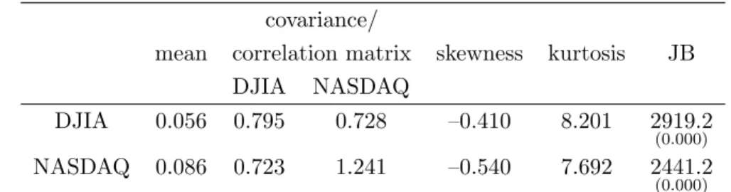
Table 2: Descriptive statistics of DJIA/NASDAQ returns over the in–sample period, 1990– 1999.
covariance/
mean correlation matrix skewness kurtosis JB DJIA NASDAQ
DJIA 0.056 0.795 0.728 –0.410 8.201 2919.2
(0.000)
NASDAQ 0.086 0.723 1.241 –0.540 7.692 2441.2
(0.000)
The top right entry of the “covariance/correlation matrix” is the correlation coefficient, and the bottom left entry is the covariance. “skewness” denotes the moment–based coefficient of skewness, γ = m3/m32/2, and “kurtosis” the moment–based coefficient of kurtosis,κ=m4/m22, wheremi=T−1 t(rt−r¯)i,i= 2,3,4, and ¯r=T−1 trt.
JB is the Jarque–Bera test for normality, based on the result that, under normality, JB =T γ2/6 +T(κ−3)2/24asy∼ χ2(2). p–values are given in parentheses.
νis a 2×1 vector of constants, andt follows a GARCH process in BEKK form as given by (9), withp=q=L= 1. All parameters are estimated simultaneously by maximum likelihood.
3.1
Estimation Results
Several versions of the general mixture GARCH model (5)–(6) with p = q = 1 have been estimated. Namely, the single–component model, which corresponds to k = 1 in (1), and which is just the standard Normal–GARCH process, has been estimated with and without imposing a symmetric reaction to negative and positive shocks. The first of these models, where θ11 = 0 in (6), will be denoted by Normal–GARCH(1,1), and the second by Normal–
AGARCH(1,1). Also, two–component models are considered with and without symmetric conditional mixture densities, i.e., with and without imposing μ1 = μ2 = 0 in (5), as well as
with and without leverage effects. To refer to these different models, we will use the typology of Table 1.
Table 3 reports likelihood–based goodness–of–fit measures for the models and their rankings with respect to each of these criteria, i.e., the value of the maximized log–likelihood function, and the AIC and BIC criteria of Akaike (1973) and Schwarz (1978), respectively. While it is not surprising that the Normal–GARCH model is the worst performer with respect to each of these criteria, several additional observations are worth mentioning. First, the normal mixture specifications allowing for asymmetric conditional densities, i.e., admitting nonzero component means in (5), are always favored against their symmetric counterparts. This is not the case when we consider the dynamic asymmetry, i.e., leverage effects. The improvement in log– likelihood is much larger when passing from the symmetric MNMS(2)–GARCH(1,1) to the MNMS(2)–AGARCH(1,1) model (difference in log–likelihood: 23.7) than when passing from
1990 1995 2000 2005 −10 −5 0 5 10 DJIA returns time 1990 1995 2000 2005 −15 −10 −5 0 5 10 15 NASDAQ returns time 0 5 10 15 20 25 −0.1 −0.05 0 0.05 0.1 lag SACF
SACF of DJIA returns, 1990−1999
0 5 10 15 20 25 −0.1 −0.05 0 0.05 0.1 lag SPACF
SPACF of DJIA returns, 1990−1999
0 5 10 15 20 25 −0.1 −0.05 0 0.05 0.1 lag SACF
SACF of NASDAQ returns, 1990−1999
0 5 10 15 20 25 −0.1 −0.05 0 0.05 0.1 lag SPACF
SPACF of NASDAQ returns, 1990−1999
in−sample period out−of−sample period out−of−sample period in−sample period
Figure 1: The top panel shows the percentage returns of the DJIA (left) and the NASDAQ (right). The middle and bottom panels show the sample autocorrelation (SACF) and partial autocorrelation functions (SPACF) over the period from 1990 to 1999 (in–sample period), respectively. Dashed lines represent approximate 95% one–at–a–time confidence intervals.
Table 3: Likelihood–based goodness of fit.
Distributional L AIC BIC
Model K Value Rank Value Rank Value Rank Normal–GARCH(1,1) 14 –5606.9 6 11241.8 6 11323.5 6 MNMS(2)–GARCH(1,1) 26 –5504.2 4 11060.5 4 11212.2 4 MNM(2)–GARCH(1,1) 28 –5482.6 3 11021.3 3 11184.7 1 Normal–AGARCH(1,1) 16 –5592.5 5 11217.0 5 11310.4 5 MNMS(2)–AGARCH(1,1) 30 –5480.5 2 11021.0 2 11196.1 3 MNM(2)–AGARCH(1,1) 32 –5467.6 1 10999.2 1 11185.9 2
The leftmost column states the type of volatility model fitted to the bivariate NASDAQ/DJIA returns. The column labeled K reports the number of parameters of a model (including the mean equation);L is the log–likelihood; AIC =−2L+ 2K; and BIC =−2L+KlogT, whereT is the number of observations. For each of the three criteria the criterion value and the ranking of the models are shown. Boldface entries indicate the best model for the particular criterion.
the asymmetric MNM(2)–GARCH(1,1) process to its AGARCH(1,1) counterpart (difference in log–likelihood: 15.1). As a consequence, the MNM(2)–GARCH(1,1) specification performs best overall according to the BIC. We note, however, that the difference in BIC for the latter two models is insignificant according to the Kass and Raftery–recommendation mentioned at the end of Section 2.1. Also, a closer inspection of the parameter estimates will reveal that the leverage effect may be an exclusive feature of the high–volatility component, so that the difference in the number of parameters between these models shrinks from four to two, which would reverse the models’ ranking. Moreover, a likelihood ratio test for θ1 = θ2 = 0, with
associated test statistic LRT = 2×(5482.6−5467.6) = 30.1, would reject at conventional critical values given by the asymptotically validχ2 distribution with four degrees of freedom, thus favoring the model with leverage effects.
The maximum likelihood estimates (MLEs) are reported in Tables 4 and 5 for the models without and with leverage effects, respectively. The functionfminunc in Matlab (version 6.5) was used to find the MLEs. We did not encounter convergence problems, and the estimates were robust with respect to different sets of starting values. As our focus is on volatility dynamics, the parameters of the mean equation (20) are not reported. Shown are the parameter matrices A
0j, A1j, and B1j, j = 1,2, of the BEKK representation (9). In addition, we report the component–specific persistence measures, i.e., the largest eigenvalues of the matrices A1j+B1j, j= 1,2, where these matrices have been recovered from the BEKK representation using (10), as well as the largest eigenvalues of the matricesC11 andC22defined in Proposition
1. The two–component models have been ordered such that λ1 > λ2. Furthermore, the
implied unconditional overall and component–specific covariance matrices and their associated correlation coefficients are shown in Table 6.
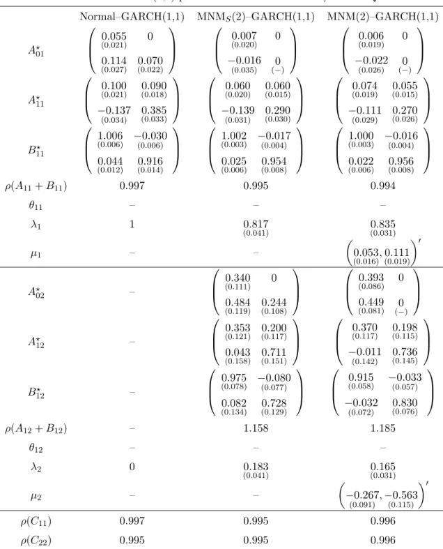
Table 4: MNM–GARCH(1,1) parameter estimates for DJIA/NASDAQ returns Normal–GARCH(1,1) MNMS(2)–GARCH(1,1) MNM(2)–GARCH(1,1)
A01 ⎛ ⎜ ⎝ 0.055 (0.021) 0 0.114 (0.027) (00..070022) ⎞ ⎟ ⎠ ⎛ ⎜ ⎝ 0.007 (0.020) 0 −0.016 (0.035) (−0) ⎞ ⎟ ⎠ ⎛ ⎜ ⎝ 0.006 (0.019) 0 −0.022 (0.026) (−0) ⎞ ⎟ ⎠ A11 ⎛ ⎜ ⎝ 0.100 (0.021) (00..090018) −0.137 (0.034) (00..385033) ⎞ ⎟ ⎠ ⎛ ⎜ ⎝ 0.060 (0.020) (00..060015) −0.139 (0.031) (00..290030) ⎞ ⎟ ⎠ ⎛ ⎜ ⎝ 0.074 (0.019) (00..055015) −0.111 (0.029) (00..270026) ⎞ ⎟ ⎠ B 11 ⎛ ⎜ ⎝ 1.006 (0.006) −(00..006)030 0.044 (0.012) (00..916014) ⎞ ⎟ ⎠ ⎛ ⎜ ⎝ 1.002 (0.003) −(00..004)017 0.025 (0.006) 0(0..954008) ⎞ ⎟ ⎠ ⎛ ⎜ ⎝ 1.000 (0.003) −(00..004)016 0.022 (0.006) (00..956008) ⎞ ⎟ ⎠ ρ(A11+B11) 0.997 0.995 0.994 θ11 – – – λ1 1 0.817 (0.041) (00..835031) μ1 – – 0.053 (0.016),0(0..111019) A02 – ⎛ ⎜ ⎝ 0.340 (0.111) 0 0.484 (0.119) 0(0..244108) ⎞ ⎟ ⎠ ⎛ ⎜ ⎝ 0.393 (0.086) 0 0.449 (0.081) (0−) ⎞ ⎟ ⎠ A12 – ⎛ ⎜ ⎝ 0.353 (0.121) 0(0..200117) 0.043 (0.158) 0(0..711151) ⎞ ⎟ ⎠ ⎛ ⎜ ⎝ 0.370 (0.117) (00..198115) −0.011 (0.142) (00..736145) ⎞ ⎟ ⎠ B12 – ⎛ ⎜ ⎝ 0.975 (0.078) −(00..077)080 0.082 (0.134) 0(0..728129) ⎞ ⎟ ⎠ ⎛ ⎜ ⎝ 0.915 (0.058) −(00.057).033 −0.032 (0.072) (00..830076) ⎞ ⎟ ⎠ ρ(A12+B12) – 1.158 1.185 θ12 – – – λ2 0 0.183 (0.041) (00..165031) μ2 – – −0.267 (0.091) ,− 0.563 (0.115) ρ(C11) 0.997 0.995 0.996 ρ(C22) 0.995 0.995 0.996
Approximate standard errors are given in parentheses. If parameters with nonnegativity restrictions were extremely close to the boundary, we reestimated the model with these parameters set to zero, so that their standard errors are not reported. This applies to the lower diagonal element ofA
01for model MNMS(2)–
GARCH(1,1), as well as to the lower diagonal elements of A
01 and A02 for model MNM(2)–GARCH(1,1). Note that matrices A
0j,A1j, and B1j,j = 1,2, correspond to the BEKK representation (9) of the model,
while matrices A1j+B1j, j = 1,2, the maximal eigenvalues of which are reported, are associated with the
vech representation (6). ρ(C11) andρ(C22) denote the largest eigenvalues of the matricesC11andC22, defined in Proposition 1, which determine whether the unconditional second and fourth moments, respectively, exist.
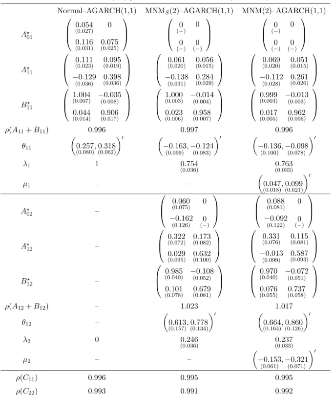
Table 5: MNM–AGARCH(1,1) parameter estimates for DJIA/NASDAQ returns
Normal–AGARCH(1,1) MNMS(2)–AGARCH(1,1) MNM(2)–AGARCH(1,1)
A01 ⎛ ⎜ ⎝ 0.054 (0.027) 0 0.116 (0.031) (00..075025) ⎞ ⎟ ⎠ ⎛ ⎜ ⎝ 0 (−) 0 0 (−) (0−) ⎞ ⎟ ⎠ ⎛ ⎜ ⎝ 0 (−) 0 0 (−) (−0) ⎞ ⎟ ⎠ A11 ⎛ ⎜ ⎝ 0.111 (0.023) 0(0..095019) −0.129 (0.036) 0(0..398036) ⎞ ⎟ ⎠ ⎛ ⎜ ⎝ 0.061 (0.020) (00..056015) −0.138 (0.031) (00..284029) ⎞ ⎟ ⎠ ⎛ ⎜ ⎝ 0.069 (0.020) 0(0..051015) −0.112 (0.028) 0(0..261026) ⎞ ⎟ ⎠ B11 ⎛ ⎜ ⎝ 1.004 (0.007) −(00..008)035 0.044 (0.014) (00..906017) ⎞ ⎟ ⎠ ⎛ ⎜ ⎝ 1.000 (0.003) −(00.004).014 0.023 (0.006) (00..958007) ⎞ ⎟ ⎠ ⎛ ⎜ ⎝ 0.999 (0.003) −(00..003)013 0.017 (0.005) (00..962006) ⎞ ⎟ ⎠ ρ(A11+B11) 0.996 0.997 0.996 θ11 0.257 (0.080),(00..318062) −0.163 (0.099) ,− 0.124 (0.083) −0.136 (0.100),− 0.098 (0.078) λ1 1 0.754 (0.036) (00..763033) μ1 – – 0.047 (0.018),(00..099021) A02 – ⎛ ⎜ ⎝ 0.060 (0.075) 0 −0.162 (0.126) (−0) ⎞ ⎟ ⎠ ⎛ ⎜ ⎝ 0.088 (0.081) 0 −0.092 (0.122) (0−) ⎞ ⎟ ⎠ A 12 – ⎛ ⎜ ⎝ 0.322 (0.072) (00..173082) 0.029 (0.095) (00..632100) ⎞ ⎟ ⎠ ⎛ ⎜ ⎝ 0.331 (0.076) 0(0..115081) −0.013 (0.099) 0.587 (0.093) ⎞ ⎟ ⎠ B12 – ⎛ ⎜ ⎝ 0.985 (0.040) −(00.052).108 0.101 (0.078) (00..679081) ⎞ ⎟ ⎠ ⎛ ⎜ ⎝ 0.970 (0.040) −(00..051)072 0.076 (0.055) (00..737058) ⎞ ⎟ ⎠ ρ(A12+B12) – 1.023 1.017 θ12 – 0.613 (0.157),(00..778134) 0.664 (0.164),(00..860126) λ2 0 0.246 (0.036) (00..237033) μ2 – – −0.153 (0.061),−(00.071).321 ρ(C11) 0.996 0.995 0.995 ρ(C22) 0.993 0.991 0.992
Approximate standard errors are given in parentheses. If parameters with nonnegativity restrictions were extremely close to the boundary, we reestimated the model with these parameters set to zero, so that their standard errors are not reported. This applies, for models MNMS(2)–AGARCH(1,1) and MNM(2)–AGARCH(1,1), to the diagonal
elements ofA01and to the lower diagonal element ofA02. Note that, when both diagonal elements ofA01are set to zero, the sign of the bottom left element is not identified, and, consequently, given its closeness to the boundary (zero), it was likewise fixed to zero. See the legend of Table 4 for further explanations.
Table 6: Unconditional (component–specific) covariance matrices and implied correlations. Model Normal–GARCH(1,1) MNMS(2)–GARCH(1,1) MNM(2)–GARCH(1,1) E(tt) 0.900 0.723 0.781 1.297 0.793 0.704 0.686 1.197 0.782 0.696 0.671 1.190 E(H1t) – 0.536 0.624 0.435 0.907 0.549 0.624 0.433 0.876 E(H2t) – 1.942 0.822 1.808 2.490 1.877 0.800 1.698 2.401 Model Normal–AGARCH(1,1) MNMS(2)–AGARCH(1,1) MNM(2)–AGARCH(1,1) E(tt) 0.854 0.716 0.734 1.230 0.701 0.689 0.583 1.023 0.695 0.685 0.547 0.918 E(H1t) – 0.470 0.607 0.375 0.812 0.463 0.600 0.338 0.685 E(H2t) – 1.408 0.796 1.220 1.668 1.412 0.786 1.157 1.535 The table reports the unconditional overall and component–specific covariance matrices of the error term t, as implied by the parameter estimates given in Tables 4 and 5. The associated correlation coefficients
are shown in upper triangular parts of the respective matrices.
In discussing the parameter estimates, we first draw attention to a common characteristic of all mixture models, irrespective of their allowance for asymmetry and/or leverage: All these models identify two components with distinctly different volatility dynamics. More precisely, the first component, i.e., the component with the larger mixing weight, is stationary in the sense thatρ(A11+B11)<1, and it has less weight on the reaction parameters inA11and more
weight on the persistence parameters inB11, relative to the second component. An inspection
of Table 6 also shows that Components 1 and 2 can be characterized as low– and high–volatility components, respectively. The latter is nonstationary in the sense that ρ(A12+B12)>1, and
it has considerably more weight on the reaction and less on the persistence parameters. This implies that the high–volatility component reacts more strongly to shocks, but has a shorter memory. However, all estimated mixture models are stationary in the aggregate with finite fourth unconditional moments, because, for all models, the largest eigenvalues of the matrices C11 and C22, defined in (13) and (14), respectively, are less than unity. Another observation
arising from Table 6 is that the correlations are higher in turbulent markets, i.e., in the high– volatility component, a phenomenon that has recently been investigated, among others, by Ang and Chen (2002) and Patton (2004). An informal comparison of Table 6 with columns 3–4 of Table 2 also shows that all models fit the unconditional covariance/correlation structure reasonably well, although the mixture models with a leverage effect do slightly worse in this regard.
GARCH(1,1) model in Table 4 and the MNM(2)–AGARCH(1,1) model in Table 5, the low– volatility component is associated with positive means, and the high–volatility component is associated with statistically significant negative means for both indices, implying that the low– and high–volatility components can be interpreted as bull and bear markets, respectively. A similar finding holds for the leverage effects, i.e., the dynamic asymmetries in the GARCH structure, as reported in Table 5. For both mixture AGARCH models, a leverage effect seems to be present mainly in the high–volatility, bear market component. The leverage parameters in the first component,θ11, are negative, and thus seem to indicate a “reverse” leverage effect,
but they are also insignificant statistically. On the other hand, the leverage parameters of the nonstationary component, θ12, are rather large, compared to those of the fitted Normal–
AGARCH model, indicating a very strong negative relation between current returns and future volatility. It is also interesting to note that the introduction of the leverage effects reduces the persistence measure of the high–volatility component somewhat, i.e., ρ(A12+B12) decreases.
(Note, however, that the interpretation of ρ(A12+B12) as a persistence measure is a little
awkward whenρ(A12+B12)>1.) However, at the same time, its mixing weight,λ2, increases,
so that the overall persistence of the model, as measured by ρ(C11), remains approximately
unchanged.
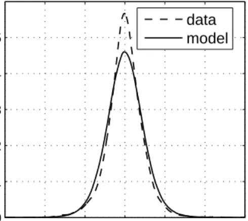
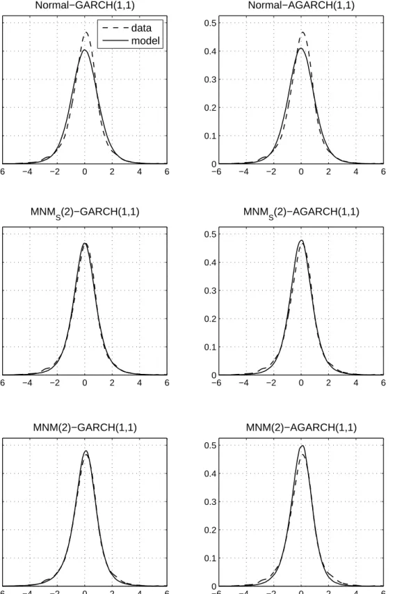
To assess the models’ fit of the unconditional distribution, Figures 2 and 3 present the empirical densities of the residuals for the DJIA and the NASDAQ, respectively, as obtained via kernel density estimation (see, e.g., Silverman, 1986), along with kernel estimates of sim-ulated samples of length 1,000,000 from the estimated models. The kernel estimator is given byfi(x) = (T h)−1tT=1K[(x−it)/h],i= DJIA, NASDAQ, where we use a Gaussian kernel, i.e., K(x) = (2π)−1/2exp{−x2/2}, and h = 1.06σiT−1/5, where σi is the respective sample standard deviation. While it is usually difficult to see the fatter tails in such figures, it is appar-ent that the empirical density is remarkably more peaked than the unconditional distribution implied by the single–regime Normal–GARCH(1,1) process, while the mixture models provide a much closer approximation to the empirical densities. Recall that the leptokurtosis observed in financial time series includes both peakedness and tailedness. In fact, both features reflect the same phenomenon, because, as noted by Ruppert (1987), if one moves probability mass from the shoulders of a distribution to the tails, then to keep the scale fixed one must also move mass from the shoulders to the center.
Finally, Figures 4 and 5 show the empirical autocorrelations of the squared residuals for the two series, along with their theoretical counterparts implied by the six estimated GARCH models. As often observed in the literature since Ding et al. (1993) and Ding and Granger (1996), the empirical autocorrelations decay rapidly at the beginning and then decrease rather
−6 −4 −2 0 2 4 6 0 0.1 0.2 0.3 0.4 0.5 Normal−GARCH(1,1) −6 −4 −2 0 2 4 6 0 0.1 0.2 0.3 0.4 0.5 MNM S(2)−GARCH(1,1) −6 −4 −2 0 2 4 6 0 0.1 0.2 0.3 0.4 0.5 0.6 MNM(2)−GARCH(1,1) −6 −4 −2 0 2 4 6 0 0.1 0.2 0.3 0.4 0.5 Normal−AGARCH(1,1) −6 −4 −2 0 2 4 6 0 0.1 0.2 0.3 0.4 0.5 MNM S(2)−AGARCH(1,1) −6 −4 −2 0 2 4 6 0 0.1 0.2 0.3 0.4 0.5 0.6 MNM(2)−AGARCH(1,1) data model
Figure 2: Kernel density estimates for the DJIA errors. Shown are, for each fitted GARCH model, kernel density estimates for the estimated empirical DJIA errors in (20) (dashed line), along with kernel estimates for the error distributions implied by the respective models (solid line), as obtained from simulated samples of length 1,000,000.
−6 −4 −2 0 2 4 6 0 0.1 0.2 0.3 0.4 0.5 Normal−GARCH(1,1) −6 −4 −2 0 2 4 6 0 0.1 0.2 0.3 0.4 0.5 MNM S(2)−GARCH(1,1) −6 −4 −2 0 2 4 6 0 0.1 0.2 0.3 0.4 0.5 MNM(2)−GARCH(1,1) −6 −4 −2 0 2 4 6 0 0.1 0.2 0.3 0.4 0.5 Normal−AGARCH(1,1) −6 −4 −2 0 2 4 6 0 0.1 0.2 0.3 0.4 0.5 MNM S(2)−AGARCH(1,1) −6 −4 −2 0 2 4 6 0 0.1 0.2 0.3 0.4 0.5 MNM(2)−AGARCH(1,1) data model
Figure 3: Kernel density estimates for the NASDAQ errors. Shown are, for each fitted GARCH model, kernel density estimates for the estimated empirical NASDAQ errors in (20) (dashed line), along with kernel estimates for the error distributions implied by the respective models (solid line), as obtained from simulated samples of length 1,000,000.
slowly, with the NASDAQ exhibiting more significant lags than the DJIA. While the single– regime models fail to capture this pattern, the mixture models tend to do better in this regard. However, the mixture models with leverage effects, with the exception of MNMS(2)– AGARCH(1,1) in case of the NASDAQ, suffer from the autocorrelations being much too small at the beginning. Overall, models MNMS(2)–GARCH(1,1) and MNM(2)–GARCH(1,1) provide the best fit to the empirical autocorrelations of the squares, which can presumably be explained by the reasoning at the end of Section 2.3.
3.2
Application to Value–at–Risk
In this section, we evaluate the models’ capability to accurately measure the out–of–sample Value–at–Risk (VaR) of portfolios formed from the stock indices under investigation. In Section 3.2.1 we discuss methods for evaluating the VaR measures provided by the respective models, and Section 3.2.2 presents the empirical results.
3.2.1 Backtesting Value–at–Risk Measures
VaR is a widely employed tool in risk management (e.g., Christoffersen and Pelletier, 2004), and it can briefly be defined as follows. For a given model, the VaR at level ξ for period t, denoted by VaRt(ξ), is implicitly defined by F(VaRt(ξ)|Ψt−1) = ξ, where F(·|Ψt−1) is the conditional cumulative distribution function (cdf) of the portfolio return, rp,t, implied by the model under consideration. A violation or hit is said to occur at time t if rp,t < VaRt(ξ). To test the models’ suitability for calculating accurate ex–ante VaR measures, we define the binary sequence It = ⎧ ⎪ ⎨ ⎪ ⎩ 1, if rp,t<VaRt, 0, if rp,t≥VaRt. (21)
Then the empirical shortfall probability is ξ = x/T, where x = Tt=1It is the number of observed violations, and T is the number of forecasts evaluated. Two tests on the sequence (21) will be conducted, which can be characterized as tests for correct unconditional and conditional coverage, respectively.
For the first test, based on ideas of Kupiec (1995), we note that, from both the risk management and the regulatory perspective, the main interest is often whether a model’s actual shortfall probability is greater than the target probability ξ. Therefore, the check whether ξ is significantly larger than ξ is conducted using a one–sided binomial test, where
0 50 100 150 −0.05 0 0.05 0.1 0.15 0.2 Normal−GARCH(1,1) lag
ACF
0 50 100 150 −0.05 0 0.05 0.1 0.15 0.2 Normal−AGARCH(1,1) lagACF
0 50 100 150 −0.05 0 0.05 0.1 0.15 0.2 MNM S (2)−GARCH(1,1) lag 0 50 100 150 −0.05 0 0.05 0.1 0.15 0.2 MNM S (2)−AGARCH(1,1) lag 0 50 100 15 0 −0.05 0 0.05 0.1 0.15 0.2 MNM(2)−GARCH(1,1) lag 0 50 100 15 0 −0.05 0 0.05 0.1 0.15 0.2 MNM(2)−AGARCH(1,1) lag Figure 4: Sho wn are empirical and m o d el–implied theoretical (b o ld line) auto correlations of the squared errors for the DJIA. Dashed lines represen t a ppro x imate 9 5% one–at–a–time confidence in terv a ls.0 50 100 150 −0.05 0 0.05 0.1 0.15 0.2 0.25 0.3 Normal−GARCH(1,1) lag
ACF
0 50 100 150 −0.05 0 0.05 0.1 0.15 0.2 0.25 0.3 Normal−AGARCH(1,1) lagACF
0 50 100 150 −0.05 0 0.05 0.1 0.15 0.2 0.25 0.3 MNM S (2)−GARCH(1,1) lag 0 50 100 150 −0.05 0 0.05 0.1 0.15 0.2 0.25 0.3 MNM S (2)−AGARCH(1,1) lag 0 50 100 15 0 −0.05 0 0.05 0.1 0.15 0.2 0.25 0.3 MNM(2)−GARCH(1,1) lag 0 50 100 15 0 −0.05 0 0.05 0.1 0.15 0.2 0.25 0.3 MNM(2)−AGARCH(1,1) lag Figure 5: Sho wn are empirical and m o d el–implied theoretical (b o ld line) auto correlations o f the squared errors for the NASD A Q. Dashed lines represen t a ppro x imate 95% one–at–a–time confidence in terv a ls.the p–values are calculated by p= T i=x T i ξi(1−ξ)T−i. (22)
If, according to (22), ξ is significantly larger than ξ, then the model under investigation on average tends to underestimate the risk of the financial position. However, as stressed by Christoffersen (1998) and Lopez (1999), a satisfactory backtesting method should be able to detect both deviations from the unconditional nominal shortfall probability, ξ, as well as violation clustering. For example, a VaR model that fails to appropriately account for higher– order dynamics in the return density (e.g., ARCH effects) may be correct on average (have unconditional shortfall probabilityξ), but in any given period will have uncorrect probability of violation, leading to violation clustering. See, however, Jorion (2002) for a skeptical discussion of the economic significance of violation clustering.
A duration–based backtesting approach which allows to detect rather general deviations from independence of the sequence (21) has recently been developed by Christoffersen and Pelletier (2004). Statistically, correct conditional coverage implies that the sequence {It} defined in (21) is a random sample from a Bernoulli distribution with probability (of violation) parameterξ, which in turn implies that the number of days between two violations is geometric. More formally, define the duration of time in days between two violations as
Di=ti−ti−1, (23)
whereti denotes the day of violation numberi. Then, for a correctly specified VaR model, the probability density function of the duration is given by
fG(d;ξ) = (1−ξ)d−1ξ, d∈N. (24) The geometric distribution is characterized unambiguously by its “lack of memory” property (cf. Rohatgi, 1976, p. 191), which means that the probability of observing a hit today does not depend on the number of days elapsed since the last violation. The statistical concept for characterizing the memory of a lifetime distribution is the hazard function,λ(d), which, in the discrete framework, is defined to be the conditional probability of a violation on day d given that d−1 days have passed without a violation, that is,
λ(d) := Pr(D=d|D≥d) = Pr(D=d) Pr(D≥d) = f(d) ∞ j=df(j) = f(d) S(d), (25)
where S(d) := Pr(D ≥ d) denotes the survivor function. The “lack of memory” property of the geometric distribution (24) is associated with a constant hazard function, i.e., λG(d) =ξ
for alld≥1. In contrast, violation clustering corresponds to a decreasing hazard function (or negative duration dependence), implying that the probability of a no–hit spell ending shortly decreases as the spell increases in length. Christoffersen and Pelletier (2004) propose to test the iid–ness of the binary sequence (21) via the “lack of memory” property of the sequence of durations defined in (23). The approach is to specify a lifetime distribution with a flexible hazard function that nests the geometric, so that the “lack of memory” property can be tested by means of likelihood ratio (LR) tests. See Kiefer (1988) and Christoffersen and Pelletier (2004) for a discussion of how to construct the likelihood function in the case of censored spells.
In the applications of their approach, Christoffersen and Pelletier (2004) use the continuous analogue of (24), i.e., the exponential distribution, which, for testing, can be nested in the continuous Weibull distribution. As shown by Haas (2006), however, tests based on a discrete analogue of the continuous Weibull nesting the geometric (24) have (often considerably) more power to detect violation clustering, and, therefore, we employ the discrete Weibull distribution of Nakagawa and Osaki (1975), given by the probability density function
fDW(d;a, b) = exp{−ab(d−1)b} −exp{−abdb}, a, b >0, d∈N, (26) with distribution, survivor, and hazard functions given by FDW(d;a, b) = 1−exp{−abdb}, SDW(d;a, b) = exp{−ab(d−1)d}, and λDW(d) = 1−exp{−ab[db−(d−1)b]}, respectively. The geometric (24) is nested in (26) forb= 1 and ξ= 1−exp{−a}, and (26) has decreasing (increasing) hazard ifb <1 (b >1). Thus, the hypothesis of a correct conditional (cc) shortfall probability ξ implies a simultaneous test of
H0,cc:b= 1 and a=−log(1−ξ). (27) As pointed out by Christoffersen and Pelletier (2004), although the large–sample properties of the LR test are known, they may not lead to reliable inference in particular for small VaR levels, because, even if the return series is reasonably long, the associated series of durations will be rather short due to the scarcity of violations. Thus, for controlling the size of the tests, the Monte Carlo technique of Dufour (2006) is adopted for calculating p–values. To implement this technique, we first generate N independent realizations of the LR test statistic, LRi,
i = 1, . . . , N, under the null hypothesis, i.e., using durations constructed from independent
Bernoulli hit sequences, where we use N = 9,999. We denote by LR0 the value of the test
statistic obtained for the original sample. As there are no nuisance parameters under the null hypothesis, the only complication is that the test statistics derived from binary sequences such as (21) are discrete random variables, i.e., it may happen that LRi = LR0 for some i,
1 ≤ i ≤ N. Thus, we need a rule to break ties between the test value obtained from the original sample and those obtained from Monte Carlo simulation under the null hypothesis. As shown by Dufour (2006), in this situation, the Monte Carlo p–values can be calculated as follows. For each test statistic, LRi, i= 0, . . . , N, draw a random variable, Ui, i= 0, . . . , N, which is independently uniformly distributed over the interval (0,1). The Monte Carlop–value, pN(LR0), is then given by pN(LR0) = NGN (LR0) + 1 N+ 1 , where GN(LR0) = 1− 1 N N i=1 1(LRi≤LR0) + 1 N N i=1 1(LRi=LR0)1(Ui≥U0),
and1(A) is the indicator function associated with statementA, i.e.,1(A) = 1 ifAis true and
1(A) = 0 otherwise.
3.2.2 Empirical Results
In our application, we calculate one–step–ahead out–of–sample VaR measures and consider the VaR levels ξ= 0.0025,0.005,0.01,0.025, and 0.05. The parameter estimates are updated (approximately) every month (i.e., 20 trading days) employing a moving window of data, i.e., using the most recent 2,527 observations in the sample. In this manner, we obtain, for each model, 1,947 one–step–ahead out–of–sample VaR measures.
In addition to the six GARCH models considered above, we also include the RiskMetrics model into the comparison, which, as a benchmark, has gained some popularity among risk management practitioners (JP Morgan, 1996). This model assumes that the conditional return distribution is normal with a covariance matrixHtdriven by an exponentially weighted moving average of past shocks,
Ht=λHt−1+ (1−λ)t−1t−1= (1−λ)
∞
i=1
λi−1t−it−i, (28)
whereλ is fixed at 0.94 for daily data. To make the models comparable, we couple (28) with an AR(1) process for the conditional mean as in (20), where the parameters are estimated via a simple least squares regression.
To select economically reasonable portfolios, we assume that the preferences of the investor can be characterized by an exponential expected utility function of the form
wherec is the coefficient of constant absolute risk aversion, andrp,t is the portfolio return at time t, i.e., rp,t=wtr1t+ (1−wt)r2t, wherewt is the portfolio weight of the DJIA at time t. We note that, due to our use of continuously compounded returns, the linear relation between the returns of the individual indices and the portfolio return is only an approximation. For daily returns, however, this approximation is usually rather accurate and standard practice; for discussion, see, e.g., Fama (1976, Ch. 1). For a Gaussian investor with predictive density rt|Ψt−1 ∼N(μt, Ht), whereμt = (μ1t, μ2t), andHt = (hij,t)i,j=1,2, the optimal portfolio weight in periodtis given by wt= h h22,t−h12,t 11,t+h22,t−2h12,t + 1 c μ1t−μ2t h11,t+h22,t−2h12,t. (30) Note that the first term on the right–hand side of (30) represents the global minimum variance portfolio (GMVP). Expected utility of a mixture investor with predictive density rt|Ψt−1 ∼
λ1tN(μ1t, H1t) +λ2tN(μ2t, H2t) is given by E[U(rp,t)|Ψt−1] =−λ1texp −cw˜tμ1t+ c 2 2w˜ tH1tw˜t −λ2texp −cw˜tμ2t+ c 2 2w˜ tH2tw˜t , (31) where ˜wt = (wt,1−wt). As the portfolio problem of the mixture investor does not admit a closed–from solution, we use the Newton–Raphson method to find the portfolio weight which maximizes (31). To account for different risk attitudes, we do the computations for values of cin (29) ranging from 0.1 to 1.5. Further increasingcdid not result in any notable differences compared toc= 1.5.
The results are reported in Tables 7 and 8 for the tests for unconditional and conditional coverage, respectively. In Table 7, for each value of risk aversion,c, and VaR level,ξ, we show the empirical percentage shortfall probability 100×ξ of the respective models, as well as the mean absolute error (MAE) over the different c–values, given by MAE(ξ) = (1/6)6i=1|ξ−
ξ(ci)|, where ξ(ci) is the empirical shortfall probability associated with the ith value of c,
i = 1, . . . ,6. In Table 8, as the parameter a of the discrete Weibull distribution (26) is not
easily interpretable for b = 1, we report, along with the estimated memory parameterb, the quantity 100/E(D), where E(D) is the mean duration implied by the fitted discrete Weibull, i.e., E(D) = ∞d=1dfDW(d;a, b) = ∞d=0(1−FDW(d;a, b)) = d∞=0exp{−abdb}, which may
serve as an estimate for the unconditional percentage shortfall probability.
Tables 7 and 8 show, in accordance with earlier results (e.g., Diebold et al., 1999), that the RiskMetrics model (28) is clearly not appropriate, as it significantly underestimates the VaR at all levels. The single–component GARCH(1,1) models, although much better than the RiskMetrics specification, are likewise inadequate in particular for the lower VaR levels, i.e.,
the more extreme risks. They do reasonably well for the higher levelsξ= 0.025 and 0.05. This is reconcilable with the occasionally expressed view that normality may be an appropriate assumption for everyday risks, given that, for example, the VaR at level 0.05 is expected to be violated once every month.
The best results with respect to unconditional coverage, as reported in Table 7, are obtained for the mixture model with an asymmetric conditional density and without leverage, i.e., model MNM(2)–GARCH(1,1), although model MNM(2)–AGARCH(1,1) also performs reasonably well. It thus appears that, in the context of the mixture models, capturing the asymmetries in the conditional density is much more important than accounting for dynamic asymmetries in the conditional variance. This may appear somewhat surprising in view of the in–sample significance of the leverage terms reported in Table 3, but the finding is similar to earlier results such as those of Loudon et al. (2000), who compare a number of both symmetric and asymmetric univariate GARCH models when applied to British stock returns. They find that the parameters governing the asymmetric response to negative and positive shocks are all highly significant in–sample, but the out–of–sample performance of symmetric and asymmetric models is fairly similar. Note, however, that an at least moderate improvement when allowing for leverage effects is observed within the class of single–component Normal–GARCH(1,1) models.
A comparison of the results for the duration–based tests in Table 8 with those in Ta-ble 7 reveals that violation clustering, in general, seems to be not a serious proTa-blem, al-though, for all models, the estimated memory parameter, b, tends to be (often slightly) be-low unity, thus indicating mild deviations from the geometric distribution. As before, mod-els MNM(2)–GARCH(1,1) and MNM(2)–AGARCH(1,1) exhibit the best fit. However, while model MNM(2)–GARCH(1,1) passes the test for correct unconditional coverage for all (c, ξ)– combinations, the hypothesis of correct conditional coverage is now rejected in two cases. In particular, the estimated value ofb= 0.61 forc= 0.1 andξ= 0.01 indicates a relatively strong clustering of violations, leading to a rejection at the 1% level. Similarly, significant violation clustering is detected for severalc–values at the 5% VaR level for the Normal–AGARCH(1,1) model, where the duration–based test, in contrast to the results in Table 7, rejects the hypoth-esis of a correctly specified VaR model.
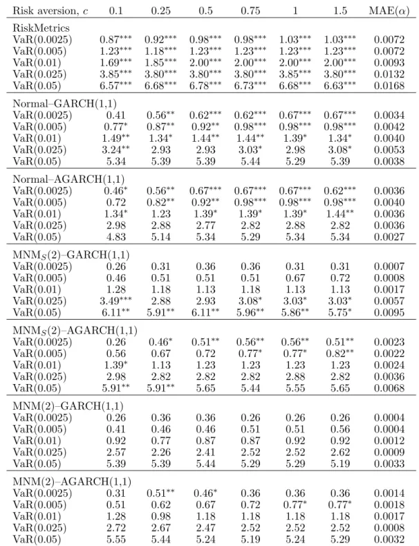
Table 7: Evaluation of Value–at–Risk (VaR) measures: Unconditional coverage (100×ξ). Risk aversion,c 0.1 0.25 0.5 0.75 1 1.5 MAE(α) RiskMetrics VaR(0.0025) 0.87∗∗∗ 0.92∗∗∗ 0.98∗∗∗ 0.98∗∗∗ 1.03∗∗∗ 1.03∗∗∗ 0.0072 VaR(0.005) 1.23∗∗∗ 1.18∗∗∗ 1.23∗∗∗ 1.23∗∗∗ 1.23∗∗∗ 1.23∗∗∗ 0.0072 VaR(0.01) 1.69∗∗∗ 1.85∗∗∗ 2.00∗∗∗ 2.00∗∗∗ 2.00∗∗∗ 2.00∗∗∗ 0.0093 VaR(0.025) 3.85∗∗∗ 3.80∗∗∗ 3.80∗∗∗ 3.80∗∗∗ 3.85∗∗∗ 3.80∗∗∗ 0.0132 VaR(0.05) 6.57∗∗∗ 6.68∗∗∗ 6.78∗∗∗ 6.73∗∗∗ 6.68∗∗∗ 6.63∗∗∗ 0.0168 Normal–GARCH(1,1) VaR(0.0025) 0.41 0.56∗∗ 0.62∗∗∗ 0.62∗∗∗ 0.67∗∗∗ 0.67∗∗∗ 0.0034 VaR(0.005) 0.77∗ 0.87∗∗ 0.92∗∗ 0.98∗∗∗ 0.98∗∗∗ 0.98∗∗∗ 0.0042 VaR(0.01) 1.49∗∗ 1.34∗ 1.44∗∗ 1.44∗∗ 1.39∗ 1.34∗ 0.0040 VaR(0.025) 3.24∗∗ 2.93 2.93 3.03∗ 2.98 3.08∗ 0.0053 VaR(0.05) 5.34 5.39 5.39 5.44 5.29 5.39 0.0038 Normal–AGARCH(1,1) VaR(0.0025) 0.46∗ 0.56∗∗ 0.67∗∗∗ 0.67∗∗∗ 0.67∗∗∗ 0.62∗∗∗ 0.0036 VaR(0.005) 0.72 0.82∗∗ 0.92∗∗ 0.98∗∗∗ 0.98∗∗∗ 0.98∗∗∗ 0.0040 VaR(0.01) 1.34∗ 1.23 1.39∗ 1.39∗ 1.39∗ 1.44∗∗ 0.0036 VaR(0.025) 2.98 2.88 2.77 2.82 2.88 2.82 0.0036 VaR(0.05) 4.83 5.14 5.34 5.29 5.34 5.34 0.0027 MNMS(2)–GARCH(1,1) VaR(0.0025) 0.26 0.31 0.36 0.36 0.31 0.31 0.0007 VaR(0.005) 0.46 0.51 0.51 0.51 0.67 0.72 0.0008 VaR(0.01) 1.28 1.18 1.13 1.18 1.13 1.13 0.0017 VaR(0.025) 3.49∗∗∗ 2.88 2.93 3.08∗ 3.03∗ 3.03∗ 0.0057 VaR(0.05) 6.11∗∗ 5.91∗∗ 6.11∗∗ 5.96∗∗ 5.86∗∗ 5.75∗ 0.0095 MNMS(2)–AGARCH(1,1) VaR(0.0025) 0.26 0.46∗ 0.51∗∗ 0.56∗∗ 0.56∗∗ 0.51∗∗ 0.0023 VaR(0.005) 0.56 0.67 0.72 0.77∗ 0.77∗ 0.82∗∗ 0.0022 VaR(0.01) 1.39∗ 1.13 1.23 1.23 1.23 1.23 0.0024 VaR(0.025) 2.98 2.82 2.82 2.82 2.88 2.82 0.0036 VaR(0.05) 5.91∗∗ 5.91∗∗ 5.65 5.44 5.55 5.65 0.0068 MNM(2)–GARCH(1,1) VaR(0.0025) 0.26 0.36 0.36 0.26 0.26 0.26 0.0004 VaR(0.005) 0.41 0.46 0.46 0.51 0.51 0.56 0.0004 VaR(0.01) 0.92 0.77 0.87 0.87 0.92 0.92 0.0012 VaR(0.025) 2.57 2.26 2.41 2.52 2.52 2.62 0.0009 VaR(0.05) 5.39 5.39 5.44 5.29 5.29 5.19 0.0033 MNM(2)–AGARCH(1,1) VaR(0.0025) 0.31 0.51∗∗ 0.46∗ 0.36 0.36 0.36 0.0014 VaR(0.005) 0.51 0.62 0.67 0.72 0.77∗ 0.77∗ 0.0018 VaR(0.01) 1.28 0.98 1.18 1.18 1.18 1.18 0.0017 VaR(0.025) 2.72 2.67 2.47 2.52 2.52 2.52 0.0008 VaR(0.05) 5.55 5.44 5.24 5.19 5.24 5.29 0.0032
Shown are the results of the tests for correctunconditional coverage of out–of–sample Value–at–Risk (VaR) measures. “VaR(ξ)” refers to the VaR measures for a nominal shortfall probabilityξimplied by the respective models. Reported are the empirical percentage shortfall probabilities, 100×ξ= 100×x/T, observed for a nominal VaR levelξ,ξ= 0.0025,0.005,0.01,0.025,0.05, wherexis the empirical shortfall frequency, and T is the number of forecasts evaluated. Asterisks ∗, ∗∗ and∗∗∗ indicate significance at the 10%, 5% and 1% levels, respectively, as obtained from the one–sided binomial test (22). For each model and each nominal VaR level, ξ, “MAE(ξ)” is the mean absolute error (MAE) over the different levels of risk aversion,c, i.e., MAE(ξ) = (1/6) 6i=1|ξ−ξ(ci)|, where (c1, c2, c3, c4, c5, c6) =
T a ble 8 : E v a luation o f V alue–at–Risk (V aR) m easures: Duration–based tests (100 / E( D ) ,b ). Risk a v ersion, c 0.1 0 .25 0 .5 0.75 1 1 .5 RiskMetrics Va R (0 . 0025) (0 . 84 , 1 . 22) ∗∗∗ (0 . 88 , 1 . 02) ∗∗∗ (0 . 93 , 1 . 05) ∗∗∗ (0 . 93 , 1 . 05) ∗∗∗ (0 . 98 , 1 . 05) ∗∗∗ (0 . 98 , 1 . 05) ∗∗∗ Va R (0 . 005) (1 . 18 , 0 . 96) ∗∗∗ (1 . 12 , 0 . 92) ∗∗∗ (1 . 17 , 0 . 92) ∗∗∗ (1 . 17 , 0 . 92) ∗∗∗ (1 . 17 , 0 . 92) ∗∗∗ (1 . 17 , 0 . 92) ∗∗∗ Va R (0 . 01) (1 . 61 , 0 . 79) ∗∗∗ (1 . 79 , 0 . 87) ∗∗∗ (1 . 94 , 0 . 81) ∗∗∗ (1 . 94 , 0 . 81) ∗∗∗ (1 . 94 , 0 . 81) ∗∗∗ (1 . 94 , 0 . 81) ∗∗∗ Va R (0 . 025) (3 . 78 , 0 . 89) ∗∗∗ (3 . 74 , 0 . 95) ∗∗∗ (3 . 75 , 0 . 99) ∗∗∗ (3 . 75 , 0 . 99) ∗∗∗ (3 . 80 , 0 . 98) ∗∗∗ (3 . 75 , 0 . 98) ∗∗∗ Va R (0 . 05) (6 . 52 , 0 . 96) ∗∗∗ (6 . 61 , 0 . 92) ∗∗∗ (6 . 69 , 0 . 86) ∗∗∗ (6 . 65 , 0 . 87) ∗∗∗ (6 . 60 , 0 . 89) ∗∗∗ (6 . 56 , 0 . 90) ∗∗∗ Normal–GAR CH(1,1) Va R (0 . 0025) (0 . 35 , 0 . 82) (0 . 49 , 0 . 77) ∗∗ (0 . 55 , 0 . 89) ∗∗ (0 . 55 , 0 . 89) ∗∗ (0 . 61 , 0 . 92) ∗∗∗ (0 . 61 , 0 . 92) ∗∗∗ Va R (0 . 005) (0 . 68 , 0 . 72) ∗ (0 . 80 , 0 . 83) ∗ (0 . 86 , 0 . 88) ∗ (0 . 92 , 0 . 94) ∗∗ (0 . 92 , 0 . 94) ∗∗ (0 . 92 , 0 . 94) ∗∗ Va R (0 . 01) (1 . 39 , 0 . 77) ∗∗ (1 . 26 , 0 . 81) (1 . 37 , 0 . 83) ∗ (1 . 37 , 0 . 83) ∗ (1 . 32 , 0 . 87) (1 . 28 , 0 . 97) Va R (0 . 025) (3 . 18 , 0 . 96) (2 . 87 , 0 . 91) (2 . 85 , 0 . 86) (2 . 96 , 0 . 86) (2 . 91 , 0 . 84) (3 . 01 , 0 . 83) ∗ Va R (0 . 05) (5 . 27 , 0 . 86) (5 . 33 , 0 . 87) (5 . 33 , 0 . 87) (5 . 39 , 0 . 89) (5 . 23 , 0 . 89) (5 . 34 , 0 . 93) Normal–A GAR C H(1,1) Va R (0 . 0025) (0 . 41 , 0 . 97) (0 . 49 , 0 . 74) ∗∗ (0 . 61 , 0 . 89) ∗∗∗ (0 . 61 , 0 . 89) ∗∗∗ (0 . 61 , 0 . 89) ∗∗∗ (0 . 55 , 0 . 79) ∗∗ Va R (0 . 005) (0 . 65 , 0 . 86) (0 . 75 , 0 . 84) (0 . 87 , 0 . 98) ∗ (0 . 93 , 1 . 03) ∗∗ (0 . 93 , 1 . 03) ∗∗ (0 . 93 , 1 . 03) ∗∗ Va R (0 . 01) (1 . 27 , 0 . 92) (1 . 20 , 1 . 18) (1 . 35 , 1 . 19) (1 . 35 , 1 . 19) (1 . 36 , 1 . 28) ∗ (1 . 41 , 1 . 27) ∗ Va R (0 . 025) (2 . 90 , 0 . 87) (2 . 80 , 0 . 90) (2 . 67 , 0 . 83) (2 . 73 , 0 . 84) (2 . 79 , 0 . 86) (2 . 73 , 0 . 80) ∗ Va R (0 . 05) (4 . 75 , 0 . 89) (5 . 06 , 0 . 88) (5 . 26 , 0 . 84) ∗ (5 . 18 , 0 . 79) ∗∗ (5 . 24 , 0 . 79) ∗∗∗ (5 . 24 , 0 . 79) ∗∗∗ MNM S (2)–GAR C H(1,1) Va R (0 . 0025) (0 . 21 , 1 . 17) (0 . 23 , 0 . 72) (0 . 30 , 0 . 88) (0 . 30 , 0 . 88) (0 . 27 , 1 . 61) (0 . 27 , 1 . 61) Va R (0 . 005) (0 . 38 , 0 . 67) (0 . 47 , 1 . 09) (0 . 48 , 1 . 21) (0 . 48 , 1 . 21) (0 . 63 , 1 . 25) (0 . 67 , 1 . 10) Va R (0 . 01) (1 . 21 , 0 . 87) (1 . 12 , 0 . 86) (1 . 09 , 1 . 11) (1 . 13 , 1 . 06) (1 . 08 , 1 . 02) (1 . 08 , 1 . 05) Va R (0 . 025) (3 . 45 , 1 . 06) ∗∗ (2 . 82 , 0 . 95) (2 . 86 , 0 . 88) (3 . 02 , 0 . 90) (2 . 97 , 0 . 91) (2 . 96 , 0 . 84) ∗ Va R (0 . 05) (6 . 05 , 0 . 89) ∗∗ (5 . 85 , 0 . 89) ∗ (6 . 05 , 0 . 87) ∗∗ (5 . 89 , 0 . 87) ∗∗ (5 . 80 , 0 . 88) ∗ (5 . 70 , 0 . 90) con tin ued
T a ble 8 : E v a luation o f V alue–at–Risk (V aR) m easures: Duration–based tests (100 / E( D ) ,b ) (con tin ued). Risk a v ersion, c 0.1 0 .25 0 .5 0.75 1 1 .5 MNM S (2)–A G AR CH(1,1) Va R (0 . 0025) (0 . 21 , 1 . 11) (0 . 38 , 0 . 65) ∗∗ (0 . 44 , 0 . 71) ∗∗ (0 . 50 , 0 . 83) ∗∗ (0 . 50 , 0 . 83) ∗∗ (0 . 45 , 0 . 86) Va R (0 . 005) (0 . 50 , 0 . 79) (0 . 60 , 0 . 79) (0 . 66 , 0 . 91) (0 . 72 , 1 . 07) (0 . 72 , 1 . 07) (0 . 78 , 1 . 11) Va R (0 . 01) (1 . 32 , 0 . 87) (1 . 07 , 0 . 88) (1 . 18 , 0 . 95) (1 . 18 , 0 . 95) (1 . 18 , 0 . 95) (1 . 18 , 0 . 95) Va R (0 . 025) (2 . 92 , 0 . 93) (2 . 77 , 0 . 93) (2 . 76 , 0 . 84) (2 . 76 , 0 . 84) (2 . 81 , 0 . 85) (2 . 75 , 0 . 83) Va R (0 . 05) (5 . 85 , 0 . 92) (5 . 86 , 0 . 95) (5 . 60 , 0 . 94) (5 . 39 , 0 . 93) (5 . 49 , 0 . 93) (5 . 59 , 0 . 91) MNM(2)–GAR CH(1,1) Va R (0 . 0025) (0 . 21 , 1 . 17) (0 . 30 , 0 . 88) (0 . 30 , 0 . 88) (0 . 21 , 1 . 41) (0 . 21 , 1 . 41) (0 . 21 , 1 . 41) Va R (0 . 005) (0 . 36 , 0 . 92) (0 . 40 , 0 . 83) (0 . 40 , 0 . 83) (0 . 46 , 0 . 93) (0 . 46 , 0 . 93) (0 . 51 , 1 . 00) Va R (0 . 01) (0 . 85 , 0 . 61) ∗∗∗ (0 . 72 , 1 . 02) (0 . 83 , 1 . 04) (0 . 83 , 1 . 04) (0 . 88 , 1 . 09) (0 . 88 , 1 . 09) Va R (0 . 025) (2 . 51 , 0 . 93) (2 . 19 , 0 . 85) (2 . 34 , 0 . 81) (2 . 45 , 0 . 82) (2 . 45 , 0 . 82) (2 . 56 , 0 . 81) Va R (0 . 05) (5 . 32 , 0 . 89) (5 . 32 , 0 . 83) ∗∗ (5 . 38 , 0 . 92) (5 . 22 , 0 . 89) (5 . 21 , 0 . 85) (5 . 12 , 0 . 89) MNM(2)–A GAR C H(1,1) Va R (0 . 0025) (0 . 26 , 1 . 07) (0 . 44 , 0 . 74) ∗ (0 . 38 , 0 . 65) ∗∗ (0 . 29 , 0 . 74) (0 . 29 , 0 . 74) (0 . 29 , 0 . 74) Va R (0 . 005) (0 . 43 , 0 . 73) (0 . 55 , 0 . 86) (0 . 61 , 0 . 88) (0 . 66 , 0 . 91) (0 . 72 , 0 . 95) (0 . 72 , 0 . 95) Va R (0 . 01) (1 . 21 , 0 . 82) (0 . 92 , 0 . 86) (1 . 13 , 0 . 91) (1 . 13 , 0 . 91) (1 . 13 , 0 . 91) (1 . 13 , 0 . 91) Va R (0 . 025) (2 . 67 , 0 . 96) (2 . 62 , 0 . 92) (2 . 43 , 0 . 84) (2 . 48 , 0 . 82) (2 . 48 , 0 . 82) (2 . 48 , 0 . 81) ∗ Va R (0 . 05) (5 . 49 , 0 . 90) (5 . 40 , 0 . 99) (5 . 19 , 0 . 97) (5 . 14 , 0 . 96) (5 . 19 , 0 . 95) (5 . 24 , 0 . 93) Sho wn are the results o f the duration–based tests (27) for correct co nditional co v erage of out–of–sample V alue–at–Risk (V a R) measures. “V aR( ξ )” refers to the V aR measures for a n ominal shortfall p robabilit y ξ implied b y the resp ectiv e mo dels. R ep orted a re the p airs (100 / E( D ) ,b ), where E( D )= ∞ d=0 exp {− a bd b} is the m ean duration implied b y the estimated p arameters a and b of the d iscrete W eibull d istribution (26), applied to the sequence of durations b et w een observ ed shortfalls (23) deriv ed from the hit sequence (21), and b is the (estimated) parameter m onitoring the memory of the duration pro cess. Asterisks ∗, ∗∗ and ∗∗∗ indicate significance a t the 10%, 5 % a nd 1% lev els, resp ectiv ely , a s o btained from M on te Carlo lik elih o o d ratio tests, a s d escrib ed at the end of Section 3 .2.1.
4
Conclusions
Several extensions and modifications of the analysis conducted in this paper are worth ex-ploring. Most importantly, the unrestricted BEKK parametrization employed herein will not be suitable when the number of assets under consideration is large, because the number of parameters increases quadratically with the dimension of the return vector. The curse of di-mensionality plagues multivariate GARCH models in general, but it will appear even more burdensome in the current framework, because we have as many covariance matrices to para-meterize as we have mixture components. As noted in Section 2.2, the diagonal BEKK may be appropriate in situations with a relatively large number of assets; a recent application to a rel-atively high–dimensional problem in the framework of dynamic conditional correlation models is Cappiello et al. (2006). A perhaps more promising approach, however, which may be useful even in problems of rather high dimension, is to combine the present approach with the prin-cipal component GARCH model proposed in Alexander and Chibumba (1997) and Alexander (2001, 2002). In this context, a two–step estimation procedure suggests itself, where, on the second step, as the number of factors retained should be small, a relatively low–dimensional normal mixture GARCH model could be fitted to the factors which have been extracted on the first step as the conventional principal components. Another issue for further research is the development of easily implementable techniques for risk management and portfolio selection accommodating features such as regime–specific correlation structures and leverage effects, as documented in Section 3 of the present paper.
Acknowledgements
We are grateful for constructive comments and suggestions from two anonymous referees and the associate editor, which led to significant improvements of the paper. We also thank Matteo Bonato and participants of the 2005 NBER/NSF Satellite Workshop “Financial Risk and Time Series Analysis” in Munich and the 13th Annual Meeting of the German Finance Association in Oestrich–Winkel, 2006, for helpful discussions. The research of M. Haas was supported by the Deutsche Forschungsgemeinschaft(DFG). Part of the research of M. S. Paolella has been carried out within the National Centre of Competence in Research “Financial Valuation and Risk Management” (NCCR FINRISK), which is a research program supported by the Swiss National Science Foundation.
Appendix
In the Appendix, we derive the conditions for the moments of the MNM(k)–GARCH(1,1) model. We also provide expressions for these moments and the autocorrelation structure of the process.
A
Notation
To conveniently write down the unconditional moments of the multivariate normal mixture GARCH model, use of several patterned matrices is rather advantageous, and we define them here. A detailed discussion of (as well as explicit expressions for) these matrices can be found in Magnus (1988). The first of these matrices is the commutation matrix, Kmn, which is the mn×mn matrix with the property thatKmnvec(A) = vec(A) for everym×nmatrixA. We will use the fact that the commutation matrix allows us to transform the vec of a Kronecker product into the Kronecker product of the vecs (Magnus, 1988, Theorem 3.6). More precisely, for an m×nmatrix Aand anp×q matrix B, it is true that
vec(A⊗B) = (In⊗Kqm⊗Ip)(vecA⊗vecB). (A.1) The elimination matrix, Ln, is the n(n+ 1)/2×n2 matrix that takes away the redundant elements of a symmetric n×n matrix, i.e., for every n×n matrix A, we have Lnvec(A) = vech(A). In contrast, the duplication matrix, Dn, is the n2× n(n+ 1)/2 matrix with the property that Dnvech(A) = vec(A) for every symmetric n×nmatrix A. Its Moore–Penrose inverse,D+n, is given by D+n