A Deep Learning Framework for Optimization of
MISO Downlink Beamforming
Wenchao Xia,
Member, IEEE,
Gan Zheng,
Senior Member, IEEE,
Yongxu Zhu,
Member, IEEE,
Jun Zhang,
Member, IEEE,
Jiangzhou Wang,
Fellow, IEEE,
and Athina P. Petropulu,
Fellow, IEEE
Abstract—Beamforming is an effective means to improve the quality of the received signals in multiuser multiple-input-single-output (MISO) systems. Traditionally, finding the optimal beam-forming solution relies on iterative algorithms, which introduces high computational delay and is thus not suitable for real-time implementation. In this paper, we propose a deep learning framework for the optimization of downlink beamforming. In particular, the solution is obtained based on convolutional neural networks and exploitation of expert knowledge, such as the uplink-downlink duality and the known structure of optimal solutions. Using this framework, we construct three beamforming neural networks (BNNs) for three typical optimization problems, i.e., the signal-to-interference-plus-noise ratio (SINR) balancing problem, the power minimization problem, and the sum rate maximization problem. For the former two problems the BNNs adopt the supervised learning approach, while for the sum rate maximization problem a hybrid method of supervised and unsu-pervised learning is employed. Simulation results show that the BNNs can achieve near-optimal solutions to the SINR balancing and power minimization problems, and a performance close to that of the weighted minimum mean squared error algorithm for the sum rate maximization problem, while in all cases enjoy significantly reduced computational complexity. In summary, this work paves the way for fast realization of optimal beamforming in multiuser MISO systems.
Manuscript received March 30, 2019; revised August 2, 2019, November 4, 2019, and December 9, 2019; accepted December 11, 2019. The work of W. Xia and J. Zhang was supported in part by the National Natural Science Foundation of China (Grant No. 61871446, 61671251, U1805262, and 61404130218). The work of G. Zheng was supported in part by the UK Engineering and Physical Sciences Research Council (EPSRC, Grant No. EP/N007840/1), the Leverhulme Trust Research Project Grant (Grant No. RPG-2017-129). The work of A. P. Petropulu was supported in part by the US National Science Foundation (Grant No. CCF-1526908). We also gratefully acknowledge the support of NVIDIA Corporation with the donation of a Titan Xp GPU used for this research. This paper was presented in part at the IEEE Int. Conf. Commun. (ICC) [1], Shanghai, China, May, 2019. The associate editor coordinating the review of this paper and approving it for publication was C. Lee.(Corresponding authors: Gan Zheng; Yongxu Zhu)
W. Xia and J. Zhang are with the Jiangsu Key Laboratory of Wire-less Communications, Nanjing University of Posts and Telecommunications, and also with the Engineering Research Center of Health Service System Based on Ubiquitous Wireless Networks, Ministry of Education, Nanjing University of Posts and Telecommunications, Nanjing 210003, China (e-mail: [email protected]; [email protected]).
G. Zheng is with the Wolfson School of Mechanical, Electrical and Manufacturing Engineering, Loughborough University, Leicestershire, LE11 3TU, UK (e-mail: [email protected]).
Y. Zhu is with the Division of Computer Science and Informat-ics, London South Bank University, London, SE1 0AA, UK (e-mail: [email protected]).
J. Wang is with the School of Engineering and Digital Arts at the University of Kent, Kent, CT2 7NT, UK (e-mail: [email protected]).
A. P. Petropulu is with the Department of Electrical & Computer Engineering Rutgers, The State University of New Jersey, Piscataway, NJ 08854 (e-mail: [email protected]).
Part of this work was accepted to IEEE Int. Conf. Commun. (ICC) [1], Shanghai, China, May, 2019.
Index Terms—Deep learning, beamforming, MISO, beamform-ing neural network.
I. INTRODUCTION
Downlink beamforming techniques have attracted much attention in the past decades for their ability to realize the performance gain of multiple antennas. Beamforming has been formulated in various ways, i.e., as a signal-to-interference-plus-noise ratio (SINR) balancing problem (also known as interference balancing problem) under a total power constraint [2–4], as a power minimization problem under quality of service (QoS) constraints [5–8], or as a sum rate maximization problem under a total power constraint [2, 9–11]. Existing approaches to finding the optimal beamforming solutions heavily rely on tailor-made iterative algorithms and convex optimization, which is in turn solved by general iterative algorithms such as the interior point method. For instance, the SINR balancing problem can be solved by the iterative algorithm of [12]. The power minimization problem can be reformulated as a second-order cone programming (SOCP) [7, 8] or semidefinite programming (SDP) problem [13, 14], which can be solved directly by an optimization software package such as CVX [15]. Its optimal solution can also be obtained using iterative algorithms such as Algorithm A of [16] and the dual algorithm of [5, 12]. However, the optimal solution to the sum rate maximization problem is usually hard to obtain because the problem is nonconvex. Locally optimal solutions are obtained via iterative algorithms, such as the weighted minimum mean squared error (WMMSE) algorithm [9, 10], and asymptotically optimal solutions are obtained using the water filling algorithm combined with zero-forcing (ZF) beamforming [11].
The main drawbacks of existing iterative algorithms are the high computational complexity and the resulting latency. As a result, the beamforming technique is unable to meet the demands of real-time applications in the fifth-generation (5G) system and beyond, such as autonomous vehicles and mission critical communications. Even in non-real-time appli-cations, where the small-scale fading varies in the order of milliseconds, the latency introduced by the iterative process renders the beamforming solution outdated. To address this challenge, researchers have proposed simple heuristic beam-forming solutions which admit closed-form solutions, such as the maximum-ratio transmission beamforming, the ZF beam-forming, and the regularized ZF (RZF) beamforming. These heuristic beamforming solutions are directly computed based
on the channel state information (CSI) without iteration, and thus involve low computational delay. However, the reduction of delay is achieved at the cost of performance loss. The tradeoff between delay and performance seems to restrict the potential of the beamforming techniques and its applications in practice.
Thanks to the recent advances in deep learning (DL) tech-niques, it becomes possible to find the optimal beamforming in real time by taking into account both performance and computational delay simultaneously. This is because the DL technique trains neural networks offline and then deploys the trained neural networks for online optimization. The computa-tional complexity is transferred from the online optimization to the offline training, and only simple linear and nonlinear operations are needed when the trained neural network is used to find the optimal beamforming solution, thus greatly reducing the computational complexity and delay.
Benefiting from the development of specialized hardware, such as graphic processing units and field programmable gate arrays, DL can be implemented using these hardware resources conveniently. Accordingly, DL techniques have been widely used in many applications including wireless communications. A lot of research has attempted to use DL to address physical layer issues, including channel decoding [17, 18], detection [19–21], channel estimation [22–24], and resource manage-ment [25–32]. Among these efforts, the autoencoder based on unsupervised DL, investigated in [33, 34], is an ambitious attempt to learn an end-to-end communications system [35]. DL can also facilitate resource management [25, 26], including power allocation [27–31]. Finally, [36, 37] provide an overview on the recent advances in DL-based physical layer communi-cations and [38] suggests potential applicommuni-cations of DL to the physical layer.
However, with the exception of [39–42], there are no works focusing on beamforming design in multi-antenna communi-cations based on DL. A common method used in the related literature is codebook-based beam selection. For example, [39] designed a decentralized robust precoding scheme based on DNN in a network MIMO configuration. However, while the projection over a finite dimensional subspace reduces the diffi-culty, it also results in performance loss. [40] used a DL model to predict the beamforming matrix directly from the signals received at distributed BSs in millimeter wave systems. The sum rate performance in [40] was restricted by the quantized codebook constraint. Different from [39, 40] which predicted the beamforming matrix in the finite solution space, [41, 42] directly estimated the beamforming matrix; in that case the number of variables to predict increases significantly as the numbers of transmit antennas and users increase, leading to high training complexity of the neural networks. Furthermore, we note that none of the aforementioned works addressed the SINR balancing problem under a total power constraint, or the power minimization problem under SINR constraints.
Motivated by the above facts and the universal approxima-tion theorem [43, 44], we propose a general DL framework to achieve not only near-optimal beamforming matrix, but also reduce complexity and latency as compared to the iterative methods. Based on the proposed framework, we develop
beamforming neural networks (BNNs) to solve the three aforementioned optimization problems. Learning the optimal beamforming solution is highly nontrivial, and there are still challenges that need to be overcome in designing the BNNs. Firstly, the popular neural network software packages such as Keras and Tensorflow currently (March 2019) do not support complex numbers as input or output [35]. However, both channel and beamforming vectors are inherently complex. Naively using a black-box DL model to predict beamforming vectors based on CSI matrices (with a suitable real-valued representation) will not only lead to high complexity of pre-diction, but also lose the specific structures of the problems of interest. Secondly, the power minimization problem has strict QoS constraints and guaranteeing a feasible solution using neural networks is a challenge. In addition, different from the SINR balancing and power minimization problems, there is no practically useful algorithm that can achieve the optimal solution to the sum rate maximization problem (and other nonconvex beamforming problems), and thus the supervised learning method based on locally optimal solution cannot achieve good performance. In this paper, we will tackle these challenges, and our main contributions are summarized as follows:
• We provide a DL-based framework for the beamforming optimization in the multiple-input-single-output (MISO) downlink, where the BS has multiple antennas while each user terminal has a single antenna. The proposed framework is designed based on the CNN structure. Different from existing works where the CNN was ap-plied to power control [29, 30], resource allocation [45], and wireless scheduling [46], the proposed framework combines a signal processing module with the neural network module by exploiting expert knowledge such as the uplink-downlink duality and the known structure of the optimal solutions, so as to improve learning effi-ciency by specifying the best parameters to be learned; those parameters are typically not the direct beamforming matrix. This framework can deal with three types of beamforming optimization problems: 1) problems whose optimal solutions are easy to find and the constraints are easy to meet; 2) problems whose optimal solutions are easy to find but the constraints are hard to meet; and 3) problems which have no practically useful algorithm that can achieve optimal solutions efficiently. Under this framework, we propose three BNNs for solving three typical optimization problems in MISO systems, i.e., the SINR balancing problem under a total power constraint, the power minimization problem under QoS constraints, and the sum rate maximization problem under a total power constraint.
• In the proposed supervised BNNs for the SINR balancing and power minimization problems, instead of estimating the beamforming matrix withN K elements, whereN is the number of the transmit antennas at the BS and K
is the number of users, we exploit the uplink-downlink duality of solutions [5, 6, 12] and predict the virtual uplink power allocation vector with only K elements. Thus,
the demand on the prediction capability of the BNNs in terms of network neurons and layers is significantly reduced. Also, the training and prediction complexity and cost are reduced. In the proposed BNN for the sum rate maximization problem, we exploit the known structure of the optimal solutions and predict two power allocation vectors with a total of 2K elements. This approach still has advantages as compared to predicting the beamforming matrix directly.
• We propose a hybrid two-stage BNN with both supervised and unsupervised learning to find the beamforming solu-tion to the sum rate maximizasolu-tion problem [29], since no practically useful algorithm can find the global optimum. In the first stage, we use the supervised learning method with a mean squared error (MSE)-based loss function to make the predictions as close as possible to the WMMSE algorithm, which is known to achieve the locally optimal solution. In the second stage, we modify the metric in the loss function to be the sum rate, and update the network parameters according to the unsupervised learning method, which achieves a performance close to that of the WMMSE algorithm.
The remainder of this paper is organized as follows. Section II introduces the system model and formulates three beam-forming optimization problems in the MISO downlink. Section III provides the framework for the beamforming optimization and then Sections IV, V and VI propose the BNNs under the framework for the SINR balancing problem, the power min-imization problem, and the sum rate maxmin-imization problem, respectively. Numerical results are presented in Section VII. Finally, conclusion is drawn in Section VIII.
Notations:The notations are given as follows. Matrices and vectors are denoted by bold capital and lowercase symbols, respectively. (A)T and(A)H stand for transpose and conju-gate transpose of A, respectively. The notations || • ||1 and || • ||2arel1 andl2norm operators, respectively. The operator diag(a)denotes the operation to diagonalize the vectorainto a matrix whose main diagonal elements are from a. Finally,
a ∼ CN(0,Σ) represents a complex Gaussian vector with zero-mean and covariance matrix Σ.
II. SYSTEMMODEL
We consider a downlink transmission scenario where a BS equipped withN antennas servesKsingle-antenna users. The channel between userkand the BS is denoted ashk ∈CN×1. The received signal at userk is given by
yk=hHk K X
k0=1
wk0xk0+nk, (1) wherewkrepresents the beamforming vector for userk,xk∼ CN(0,1)is the transmitted symbol from the BS to userk, and
nk ∼ CN(0, σ2) denotes the additive Gaussian white noise (AWGN) with zero mean and varianceσ2. The received SINR of userk equals γkdl= |h H k wk|2 PK k0=1,k06=k|hHkwk0|2+σ2 . (2)
One conventional optimization problem seeks to maximize minkγkdl/ρk subject to a transmit power constraint, where
ρk’s are constant weights denoting the importance of the sub-streams. Such an optimization problem is referred to as interference or SINR balancing, and has been investigated in many works [2–4]. The SINR balancing problem is formulated as: P1: max W 1≤mink≤K γkdl ρk , s.t. K X k=1 ||wk||2≤Pmax, (3) where W = [w1,w2, . . . ,wK] is a set of beamforming vectors andPmaxis the power budget.
Another important problem is the power minimization prob-lem under a set of SINR constraints [6, 7]. A network operator may be more interested in how to minimize the transmit power while fulfilling the demands for QoS, i.e.,
P2: min W K X k=1 ||wk||2, s.t.γkdl≥Γk,∀k, (4) where Γk is the SINR constraint of user k. For ease of ref-erence, we defineΓ= [Γ1,· · ·,ΓK]T as the SINR constraint vector.
Finally, the weighted sum rate maximization problem under a total power constraint has also attracted a lot of attention [2, 9, 10]. It can be formulated as:
P3: max W K X k=1 αklog2(1 +γ dl k ), s.t. K X k=1 ||wk||2≤Pmax, (5) whereαk is a constant weight of userk.
We choose the above problems as representative examples to demonstrate the effectiveness of our proposed DL beamform-ing framework. Practical algorithms to find optimal solutions are available for P1 [8, 12, 47] and P2 [5, 7, 8, 12, 13], thus supervised learning can be adopted for those problems. In this work, for simplicity, we assume that the optimal solution to problemP2always exists and do not consider the infeasibility of QoS constraints. Under this assumption, P2 still has the additional challenge of satisfying strict QoS constraints. P3
is a difficult nonconvex problem and is usually solved using the iterative WMMSE approach [9, 10], therefore, supervised learning alone is insufficient for this case. In the rest of the paper, we will show how the solutions to these three types of problems can be efficiently learned by the proposed DL-based beamforming framework.
III. A DL-BASEDFRAMEWORK FORBEAMFORMING
OPTIMIZATION
DL-based neural networks were initially designed for solv-ing classification problems, but they can also achieve satis-factory performance in regression problems. For example, the DNN was used to predict transmit power [27, 28]. Existing works mainly take real data, such as channel gains and transmit power, as input and output, but channel and beam-forming matrices are both complex. In addition, predicting the beamforming matrix withN K elements directly may lead to inaccurate results. While we could use wider or deeper
MSE/MAE CL AC CL AC FC AC BN Output Flatten BN Input
Neural network module
I(h)
R(h)
Supervised/ unsupervised learning
Beamforming recovery module
Key
features Beamforming matrix
...
...
Expert knowledge
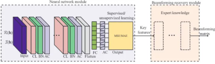
Fig. 1. A DL-based framework for the beamforming optimization in MISO downlink, which includes two main modules: the neural network module and the beamforming recovery module. The neural network module is composed of an input layer, convolutional (CL) layers, batch normalization (BN) layers, activation (AC) layers, a flatten layer, a fully-connected (FC) layer, and an output layer, whereas the key features and the functional layers in the beamforming recovery module are specified by the expert knowledge.
neural networks with more neurons to improve the learning ability, such huge networks would lead to high training and implementation complexity and their learning performance could not be guaranteed. For example, too deep or wide neural networks can cause over-fitting.
The proposed DL-based framework for the beamforming optimization in MISO downlink is shown in Fig. 1. We choose the CNN architecture as the base of the framework, because the CNN has strong ability of extracting features as well as approximation ability [43, 44]. In addition, the CNN can reduce the number of learned parameters by sharing weights and biases [30]. The proposed framework, instead of estimating the beamforming matrix directly, only predicts key features extracted from the beamforming matrix according to expert knowledge specific to the problem under consideration. Therefore, the demand for the prediction capability in terms of network neurons and layers, as well as its complexity, is significantly reduced.
A. Structure of the Proposed Framework
As illustrated in Fig. 1, the proposed framework is a gray-box approach that takes advantages of both the con-ventional signal processing and the neural network approach. The proposed framework includes two main modules: the neural network module and the beamforming recovery module. The neural network module is composed of an input layer, convolutional layers, batch normalization layers, activation layers, a flatten layer, a fully-connected layer, and an output layer, whereas key features and the functional layers in the beamforming recovery module are specified by the expert knowledge. For ease of clarification, we assume that, besides the input, output, flatten, and fully-connected layers, there are
L = |L| groups of functional layers in the neural network module and each group includes a convolutional layer, a batch normalization layer, and an activation layer. Below we give a brief introduction to these layers.
1) Input Layer: The complex channel coefficients are fed into the neural network module to predict the key features, which are not supported by the current neural network soft-ware. To deal with this issue, two data transformations are available. One is to separate the complex channel vector, for example h = [hT1,· · · ,hTK]
T ∈
CN K×1, into in-phase component R(h) and quadrature component I(h), where R(h) andI(h) contain the real and imaginary parts of each
element in h, respectively. We call this transformation I/Q transformation. Another transformation, suggested by [48], is to map the complex channel vectorhinto two real vectors P(hk) and M(hk), where the former contains the phase information and the latter includes the magnitude information of h. This transformation is referred to as P/M transfor-mation. As far as we know, there is no evidence to show which transformation is better. In this work, we adopt I/Q transformationof complex channels and formulate the input of the first convolutional layer as [R(h),I(h)]T ∈ R2×N K. Note that the samples are fed into the neural network module in batches during the training process.
2) Convolutional Layer: Each convolutional layer l ∈ L createsclconvolution kernels of sizeal×althat are convolved with the layer inputIconv,l ∈Rb
(1) l−1×b
(2)
l−1×cl−1, whereb(1)
l−1and
b(2)l−1are the height and width of the output of the convolutional layerl−1, respectively. Note thatc0= 1b
(1)
0 = 2, andb (2) 0 =
N K. The parameters of the convolution kernels, including the weights Ξl ∈ Ral×al×cl and a bias vector ξ
l ∈ Rcl×1, are
shared among different elements inIconv,l to extract features. More specifically, the output Oconv,l ∈ Rb
(1) l ×b
(2)
l ×cl of the
convolutional layer l is
Oconv,l=Conv(Iconv,l,Ξl,ξl), l∈ L, (6) where the operatorConv(·,·,·)denotes the convolution oper-ation.
3) Batch Normalization Layer: The batch normalization layers are introduced in the neural network module, which can be put before or after the activation layers [49] according to practical experience. In the proposed framework, we adopt the former where the batch normalization layers normalize the output of the convolutional layers through subtracting the batch mean and dividing by the batch standard deviation, i.e.,
Zbn,l,c[i, j] = Oconv,l,c[i, j]−µl,c p Varl,c+l,c , l∈ L, c= 1,· · · , cl, i= 1,· · ·, b(1)l , j= 1,· · ·, b(2)l (7)
where X[i, j] denotes (i, j)-th element of matrix
X, Oconv,l,c ∈ Rb (1) l ×b (2) l is the c-th slice of Oconv,l, µl,c = PF f=1 Pb (1) l i=1 Pb (2) l j=1O (f) conv,l,c[i,j] F b(1)l b(2)l and Varl,c = PF f=1 Pb (1) l i=1 Pb (2) l j=1 O (f) conv,l,c[i,j]−µl,c 2
F b(1)l b(2)l are the batch mean and variance of thec-th slice, respectively,l,cis a small float added to the variance to avoid dividing by zero, andF is the batch size. Note that such a simple normalization process may change what the layer can represent. To address this issue, two trainable parameters θl,c and βl,c are introduced to scale and shift the normalized value Zbn,l,c[i, j] as
ˆ
Zbn,l,c[i, j] = βl,cZbn,l,c[i, j] +θl,c. This “denormalization” process is allowed by changing only these two parameters, instead of changing all parameters which may lead to the instability of the neural network module. Besides, the work in [49] claimed that the batch normalization layer can reduce the probability of over-fitting, enable a higher learning rate, and make the neural network less sensitive to the initialization of weights. Note that the batch normalization layers are
element-wise functions, such that they do not change their respective input shapes.
4) Activation Layer: Since the predicted variables are con-tinuous and positive real numbers, it is suggested that the activation functions that can generate negative values, such as tanh and linear functions, should not be used in the last activation layer. The rectified linear unit (ReLU) and sigmoid functions are good choices for the last activation layer, which are given as
ReLU(z) = max(0, z)andsigmoid(z) = 1
1 +e−z, (8) respectively. The most common choice for the intermediate activation layers is the ReLU function. Note that the functions performed in the activation layers are element-wise functions, such that their outputs have the same shapes of their inputs, respectively.
5) Flatten Layer, Fully-connected Layer, and Output Layer:
The flatten layer is only used to change the shape of its input into a vector, for the fully-connected layer to interpret. The output ofc∈Rm×1 of the fully-connected layer is
ofc=Πifc+π, (9)
where ifc∈R2N KcL×1 is the input vector, Π∈
Rm×2N KcL
andπ∈Rm×1 account for the weight matrix and bias vector, respectively, andmis the number of the neurons in the fully-connected layer. The main function of the output layer is to generate the predicted results after the neural network finishes training.
Note that apart from these functional layers, the loss func-tion also plays an important role in the proposed framework, which is marked on the output layer in Fig. 1. The loss function together with the learning rate guides the learning process of the neural network. In other words, the loss function “tells” the neural network how to update its parameters. Since the output values are continuous, it is suggested to utilize the mean absolute error (MAE) or the MSE as a metric. Given the predicted results of the f-th sample in the neural network module is qˆ(f) and the target result is q(f), the MAE and MSE are defined as
MAE= 1 F K F X f=1 ||q(f)−qˆ(f)||1, (10) and MSE= 1 F K F X f=1 ||q(f)−qˆ(f)||2 2, (11)
respectively. Generally speaking, the MAE function is more robust and is not affected by outliers. On the contrary, the MSE loss function is highly sensitive to outliers in the dataset because the MSE function tries to adjust the model according to these outlier values, at the expense of other samples [50]. In this work, the training dataset is generated by simulations and outliers are not an issue. Then we choose the MSE as the loss metric because its gradient is easier to calculate than that of the MAE.
6) Beamforming Recovery Module: The beamforming re-covery module is an important component whose aim is to recover the beamforming matrix from the predicted key features at the output layer. The functional layers in the beamforming recovery module are designed according to the expert knowledge of the beamforming optimization which maps/converts the key features to the beamforming matrix. The expert knowledge is problem-dependent and has no unified form, but what is in common is that the expert knowledge can significantly reduce the number of variables to be predicted compared to the beamforming matrix. For example, the uplink-downlink duality and specific solution structures are the typical expert knowledge for beamforming optimization.
The key features should be chosen carefully to meet some constraints required by applying the universal approximation theorem [27, 43], so that a feedforward network exists which can approximate the continuous mapping from the channel coefficients to the key features. More specifically, assume that τ is a vector containing the chosen key features, the mapping functionf(•) fromhto τ, i.e., τ =f(h), should be a real-valued continuous function over a compact set. The compact set requirement holds whenever the possible values of the inputhare bounded. However, the continuity of the mapping function depends on the choice of the key features.
In next three sections we will propose three BNNs under the proposed framework for problemsP1,P2, andP3, respective-ly, and provide implementation details to show how to make use of the expert knowledge and choose the key features.
B. Computational Complexity
The computational complexity of the proposed framework involves two main tasks: the online prediction and the offline training. To the best of our knowledge, complexity analysis of the offline training is still an open issue mainly because of the complex implementation of the backpropagation process. However, since the training is performed offline, and updated at a much longer time-scale compared to the online prediction, we assume its complexity can be afforded [51]. Thus, we focus on the complexity of the online prediction. In addition, the functional layers are problem-dependent in the beamforming recovery module, so only the complexity of the neural network module is analyzed below.
Big-O notation is a common method to describe the com-plexity of an algorithm. Given there are cl kernels of size
al×al in the l-th convolutional layer, then the numbers of multiplication and addition operations of convolutional layer
l are the same and equal toa2 lb
(1)
l b
(2)
l cl−1cl. Thus, the total time complexity of all convolutional layers measured by the number of multiplications isOP l∈La2lb (1) l b (2) l cl−1cl [52]. It is known that the batch normalization layers and activation layers are element-wise functions, thus the computational com-plexity of total batch normalization layers and total activation layers in L groups is OP l∈Lb (1) l b (2) l cl . The numbers of multiplication and addition operations of the fully-connected layer are also the same and equal tob(1)L b(2)L cLm, respectively. Then the time complexity of the fully-connected layer is given as Ob(1)L b(2)L cLm
output, and flatten layers are ignored due to the simplicity of their functions. If all convolutional layers use the kernels of size 3×3 and apply stride 1 and zero padding 1, then
b(1)l = 2 and b(2)l = N K,∀l ∈ L. Based on the above analysis and assuming the parameters of the neural network module are fixed, predicting the output of the neural network module needs 2N KP
l∈L(9clcl−1+cl) + 2N KcLm+ 2m arithmetic operations including multiplications, divisions, and exponentiations, and has an approximate complexityO(N K).
IV. BNNFORSINR BALANCINGPROBLEM As mentioned above, estimating the beamforming matrix directly leads to the higher complexity of prediction due to the large amount of variables. In order to reduce the prediction complexity, we introduce a scheme which first predicts the power allocation vector as the key feature and then achieves the corresponding beamforming matrix based on the predicted results. Such a scheme is based on the expert knowledge named the uplink-downlink duality.
A. Uplink-Downlink Duality
Before we present the BNN for the SINR balancing problem
P1, we first introduce the following lemma to describe the uplink-downlink duality of problemP1[12].
Lemma 1. GivenW˜ = [ ˜w1,w˜2, . . . ,w˜K]andPmax, we have
Cdl( ˜W, Pmax) =Cul( ˜W, Pmax), (12)
where Cdl( ˜W, Pmax)and Cul( ˜W, Pmax)are given as
Cdl( ˜W, Pmax) = max p 1≤mink≤K γkdl( ˜W,p) ρk (13) s.t. ||p||1≤Pmax, ||w˜k||2= 1,∀k, and Cul( ˜W, Pmax) = max q 1≤mink≤K γul k ( ˜W,q) ρk (14) s.t.||q||1≤Pmax, ||w˜k||2= 1,∀k, respectively, with γkdl( ˜W,p) = pk|h H kw˜k|2 PK k0=1,k06=kpk0|hHk w˜k0|2+σ2 , (15) and γulk ( ˜W,q) = qk|h H k w˜k|2 PK k0=1,k06=kqk0|hHk 0w˜k|2+σ2 . (16)
Note that p = [p1, . . . , pK]T and q = [q1, . . . , qK]T are
downlink and uplink power vectors, respectively1.
Note that problem (13) is an equivalent virtual problem of problem P1 whose optimal solutions are connected by
W∗ = ˜W∗P∗ where P∗ = diag(p∗), W∗ is the optimal 1Lemma 1 can be easily extended to the case with non-identical noise power levels. More details can refer to [12].
MSE
CLBNReLU CLBNReLUFlattenFC SigmoidOutput Conversion Input
Neural network module
Scaling ݍො ݍොכ I(h) R(h) כ Supervised learning
...
Beamforming recovery module
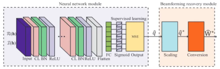
Fig. 2. BNN for the SINR balancing problem.
solution to problem P1, and W˜∗ and p∗ are the optimal solutions to problem (13). Based on Lemma 1, we find that the uplink and downlink scenarios have the same achievable SINR region and the normalized beamforming designed for the uplink reception immediately carries over to the downlink transmission [12]. Thus we first obtain the optimal power allocationq∗ and beamforming matrixW˜∗ for the easier-to-solve uplink problem (14) instead of the downlink problem (13). Then given the optimal beamforming W˜ ∗, the optimal
p∗ is obtained as the first K components of the dominant eigenvector of the following matrix [53]
Υ( ˜W∗, Pmax) = DU Dσ 1 Pmax1 TDU 1 Pmax1 TDσ , (17) where σ = σ21, 1 = [1,1, . . . ,1]T ∈ RK×1, D = diag{ρ1/|( ˜w1∗)Hh1|2, . . . , ρK/|( ˜w∗K)HhK|2}, and [U]kk0 = ( |( ˜w∗k0)Hhk|2, if k06=k, 0, else. (18)
Finally, the downlink beamforming matrix is derived asW∗= ˜
W∗P∗. Thus, instead of predictingWdirectly, we can predict the uplink power allocation vectorq. In the supervised learn-ing method, the prediction performance of the BNN depends on the quality of training samples. To generate the training samples, the optimalq∗andW˜ ∗can be found by an iterative optimization algorithm in [12, Table 1].
Note that Υ( ˜W∗, Pmax) is a non-negative matrix and the optimal objective value of problemP1is the reciprocal of the largest eigenvalue of Υ( ˜W∗, Pmax) [53]. According to the Perron-Frobenius theory, for any nonnegative real matrix Ω
with spectral radiusχ(Ω), there exist a vectorδ≥0such that
Ωδ =χ(Ω)δ [54]. Based on [12, Theorem 3], the sequence of the target value of problem P1 provided by the iterative algorithm in [12, Table 1] is strictly monotonically increasing and the largest eigenvalue of Υ( ˜W∗, Pmax)is unique. Then the corresponding eigenvector containingqis a continuous and bounded function ofhaccording to [55, Chapter 3]. Thus, we can use a neural network to approximate the mapping function fromhtoq[43].
B. BNN Structure
The proposed BNN for problem P1, shown in Fig. 2, is based on the proposed BNN framework in Fig. 1. The functions and operations of the basic layers such as the input, convolutional, batch normalization, and output layers, are the same as those in the proposed framework. Therefore, we do not explain these layers here and readers can refer to
Section III for detail. Note that in the proposed BNN for problem P1, the intermediate activation layers are fulfilled with the ReLU function whereas the last activation layer is implemented using the sigmoid function. Besides the existing layers in the framework, a scaling layer and a conversion layer are also introduced in the BNN for problemP1, which belong to the beamforming recovery module. In the following, we give the details of the scaling layer and the conversion layer.
1) Scaling Layer: Due to the existence of prediction error, it is almost impossible to guarantee that the output of the output layer always meets the power constraint in problem
P1. According to [56], the optimal solution is achieved when the equality of the constraint in problemP1holds. Therefore, we scale the results of the output layer qˆ to meet the power constraint by the following transformation,
ˆ
q∗= Pmax ||qˆ||1 ˆ
q. (19)
2) Conversion Layer: After receiving the scaled power al-location vectorqˆ∗, we can achieve the downlink beamforming matrixWˆ ∗as the final output of the BNN based onqˆ∗by the conversion layer. The beamforming recovery implemented by the conversion layer includes the following process:
1) CalculateT∗=σ2I
N+PKk=1qˆ∗khkhHk .
2) Calculate w˜∗k = w˜∗k/||w˜k∗||2,∀k, where w˜∗k = (T∗)−1h
k.
3) Find the maximal eigenvalue ψ∗max of Υ( ˜W∗, Pmax) and the associated eigenvector with respect to ψ∗max, i.e.,Υ( ˜W∗, Pmax)pˆ ∗ 1 =ψ(maxi) pˆ ∗ 1 .
4) Output Wˆ ∗ = ˜W∗Pˆ∗ as the final result where Pˆ∗ = diag(ˆp∗).
Note that the time complexity of the beamforming recovery module isO(KN2+N3+K3). In the proposed BNN for the SINR balancing problemP1, the supervised learning with the loss function based on the MSE metric is adopted.
V. BNNFORPOWERMINIMIZATIONPROBLEM Similar to the BNN for the SINR balancing problem P1, the BNN for the power minimization problem P2 obtains the downlink beamforming matrix according to the uplink-downlink duality, i.e., the expert knowledge. Specifically, we first predict the uplink power allocation vector as the key features using the trained neural network, then obtain the normalized beamforming matrix based on the predicted results. Finally, the downlink beamforming matrix is recovered from the normalized beamforming matrix by the uplink-downlink conversion method.
A. Uplink-Downlink Duality
Note that the conversion method adopted in the BNN for problemP1can not be used again, because the power budget
Pmax is unknown in the power minimization problem P2. Instead, we employ the conversion method in the following lemma [47]. MSE CL ReLU CL ReLU FC Sigmoid BN Conversion Output Flatten BN Input
Neural network module
I(h)
R(h)
ݍොכ כ
Supervised learning
...
Beamforming recovery module
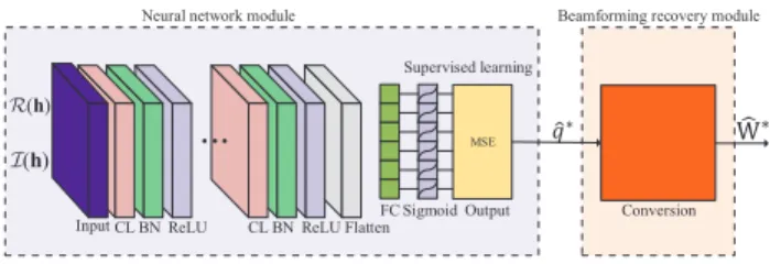
Fig. 3. BNN for the power minimization problem.
Lemma 2. Given the optimal beamforming matrix W˜ ∗ = [ ˜w∗
1, . . . ,w˜∗K]for the uplink problem 2, i.e., min q,W˜ K X k=1 qk s.t.γkul( ˜W,q)≥Γk, ||w˜k||2= 1,∀k, (20) whereγul k ( ˜W,q)is given as in(16).
The optimal beamforming vectorsw∗k,∀k, for the downlink problem P2, can be obtained by multiplying the optimal normalized beamforming vector w˜∗k by a scaling factor, i.e.,
wk∗ = p∗kw˜k∗,∀k, where p∗k is the k-th element of vector
p∗= [p∗1, . . . , p∗K]T ∈ RK×1 and p∗=σ2Ψ−11, (21) where [Ψ]kk0 = ( 1 Γk|h H k w˜∗k|2, if k=k0, −|hHk w˜∗k0|2, else. (22) The vectorp∗of the scaling factors is the optimal downlink power allocation vector. Given the optimal normalized beam-forming matrixW˜ ∗,Lemma 2allows us to achieve the opti-mal downlink power vector p∗ by (21), thenW∗ = ˜W∗P∗. Actually, if we know the uplink power allocation vectorq, the normalized beamforming matrixW˜ can be inferred as
˜ wk = T−1h k ||T−1h k||2 ,∀k, (23) whereT=σ2I
N+PKk=1qkhkhHk. Therefore, the only results that need to be predicted by the BNN is the uplink power allo-cation vectorq, which reduces significantly the computational complexity compared to the strategy that attempts to predict the beamforming matrix directly. The iterative algorithm in [5] provides a way to achieve the optimalq∗ as the training samples in the supervised learning method. Besides, such an iterative algorithm suggests the mapping function from h to
q is continuous [27, Theorem 1], so it can be approximated by a neural network.
B. BNN Structure
The BNN for problem P2 in Fig. 3 is also based on the proposed BNN framework. However, the operations of the 2In this work, for simplicity, we assume the solution to problemP2always exists. However, it can happen that the wireless network only satisfies some of the users and thus the user selection is needed. To address this issue, a possible solution is to train another neural network for user selection, and then optimize the beamforming matrix among the selected users.
conversion layer in Fig. 3 are different from those in the BNN for problem P1. After receiving the uplink power allocation vectorqˆ∗ from the output layer, the beamforming recovery in the conversion layer performs the following operations:
1) CalculateT∗=σ2I
N+PKk=1qˆ∗khkhHk .
2) Calculate w˜∗k = w˜∗k/||w˜k∗||2,∀k, where w˜∗k = (T∗)−1h
k.
3) Calculate the downlink power allocation vector pˆ∗ =
σ2(Ψ∗( ˜W∗,Γ))−11.
4) Output the downlink beamforming vectors wˆk∗ = ˆ
p∗kw˜∗k,∀k, as the final results.
Here, the time complexity of the beamforming recovery module isO(KN2+N3+K3). Note that the predicted power vectorqˆ∗by the BNN is, in general, not exact. The prediction error will lead to the inaccuracy of power allocation vectorpˆ∗ as well as the downlink beamformingWˆ∗. More specifically,
if the predicted power vector qˆ∗ has an acceptable accuracy with respect to the target power vectorq∗, i.e.,||q∗−qˆ∗||2
2< ε whereεis a small constant, then we can obtain a suboptimal solution whose objective value is larger than that of the optimal solution, i.e., PK
k=1||wˆ ∗ k||22 > PK k=1||w ∗ k||22. Intu-itively, the extra power consumptionqextra =P
K k=1||wˆ ∗ k|| 2 2− PK k=1||w∗k|| 2
2 can be regarded as the cost of the prediction error. However, if the predicted vector qˆ∗ has a significant error, i.e., ||q∗−qˆ∗||2
2 ε, the downlink beamforming Wˆ ∗ inferred from the prediction qˆ∗ may become infeasible since some elements of the vector pˆ∗ have negative values. This suggests that different from problem P1, there is a certain probability of infeasibility of the BNN prediction for problem
P2. However, our experiments show that the failure probability of the proposed BNN for problemP2is lower than1%in most settings. More details will be given in Section VII. Moreover, the supervised learning with the loss function based on the MSE metric is adopted in the proposed BNN for problemP2.
VI. BNNFORSUMRATEMAXIMIZATIONPROBLEM Different from the SINR balancing problem P1 and the power minimization problem P2, no practically useful algo-rithm is available to find the optimal solution to the sum rate maximization problemP3, for which one cannot make use of uplink-downlink duality directly. However, we will exploit a connection between problems P2 and P3 to find some key features of the optimal solution to problemP3.
A. Solution Structure
A fact was mentioned in [57] that the optimal solution to problemP2, using the minimal amount of power to achieve the given SINR targets, must meet the power constraint in problem
P3to achieve the maximal sum rate. More specifically, given the optimal transmit power P? of problem P2 and setting the total power constraint Pmax in problem P3 as P?, the SINR values of each user in problemP3can be calculated. By setting the SINR targets in problem P2with these calculated SINR values, the solutions to problemsP2andP3will be the same. According to the connection between problems P2and
P3, it has been pointed out in [2] that the optimal downlink beamforming vectors for problem P3follows the structure as
wk∗=√pk (IN+P K k=1 λk σ2hkhHk)− 1h k ||(IN +P K k=1 λk σ2hkhHk )−1hk||2 ,∀k, (24)
whereλkis a positive parameter andP K
k=1λk=P K k=1pk =
Pmax according to the strong duality of problem P2. This is because Pmax is the optimal cost function in problem P2 and PK
k=1λk is the dual function. Note that the parameter vector λ = [λ1, . . . , λK]T can be considered as a virtual power allocation vector. The solution structure in (24) provides the required expert knowledge for the beamforming design in problem P3 and λ and p are the key features. But to our best knowledge, there is no low-complexity algorithm in the literature that can find the optimal p∗k and λ∗k in (24). An improved and faster branch-and-bound algorithm was developed in [37, 51] to find the globally optimal solution, but it is mostly effective for power control problems. The WMMSE algorithm is a good choice to find the locally optimal solutions [9, 10], and such an iterative algorithm ensures the continuity of the mapping from the channel to the solution, and can be learned by a neural network [27, 30]. Therefore, we can obtain the power allocation vectorspandλaccording to the WMMSE algorithm. The supervised learning with the loss function based on the MSE metric will be first used to achieve as close to the results of the WMMSE algorithm as possible, i.e., Loss= 1 2LK L X l=1 ||p(l)−pˆ(l)||2 2+||λ (l) −λˆ(l)||2 2 , (25)
wherep(l) andλ(l) are the power vectors obtained from the WMMSE algorithm, andpˆ(l)andλˆ(l)are the predicted results of the BNN. It is worth pointing out that the results in the training samples of problems P1 and P2 are optimal, thus the MSE-based loss function is equivalent to the objective function and the supervised learning method updates network parameters towards the direction of the optimal solution. However, the WMMSE algorithm for problem P3 is locally optimal and thus (25) is not equivalent to the real objective of problemP3 which aims to maximize the weighted sum rate. To further improve the sum rate performance, we continue to train the BNN in an unsupervised learning way, whose loss function takes the objective function directly as a metric, i.e.,
Loss=− 1 2KL L X l=1 K X k=1 α(kl)log2 1 +γul,k (l). (26) B. Hybrid BNN Structure
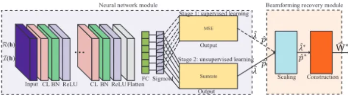
The BNN for problem P3 is presented in Fig. 4. The major difference from the BNNs in Figs. 2 and 3 is that the BNN in Fig. 4 has two stages of training. The first stage is responsible for pre-training using the supervised learning method with the loss function based on the MSE metric (25), while the second stage is responsible for enhanced training using the unsupervised learning method with the loss function whose metric is the objective function (26). Such a hybrid
MSE CL ReLU CL ReLU FC Sigmoid BN Output Flatten BN Input
Neural network module
I(h) R(h)
Sumrate Scaling Construction
Ƹ Ƹכ ߣመכ ߣመ Output ߣመƸ Stage 1: supervised learning
Stage 2: unsupervised learning
כ Beamforming recovery module
...
Fig. 4. BNN for the sum rate maximization problem.
learning method of the supervised and unsupervised learn-ing can significantly improve the learnlearn-ing performance and also accelerate convergence [29]. More specifically, the pre-training, as the approximation of WMMSE algorithm, starts with the random initialization of neural network parameters and the loss function (25). After the pre-training is finished, the neural network parameters are reserved and the loss function is replaced by (26), such that the second-stage training can achieve improved performance than the first-stage training.
Different from the BNNs in Figs. 2 and 3, the output layer in Fig. 4 generates 2K values including the power allocation vectors pˆ andλˆ. Then the scaling layer scales the results of the output layerqˆ andλˆ to meet the power constraint by the following method: ˆ p∗= Pmax ||pˆ||1 ˆ pandλˆ∗= Pmax ||λ||ˆ 1 ˆ λ. (27)
Finally, the construction layer constructs the downlink beam-forming vectors according to (24):
ˆ w∗k=ppˆ∗k (IN + PK k=1 ˆ λ∗k σ2hkhHk )−1hk ||(IN +P K k=1 ˆ λ∗ k σ2hkhHk)−1hk||2 ,∀k. (28) Thus, the time complexity of the beamforming recovery mod-ule for problem P3is O(KN2+N3).
VII. SIMULATIONRESULTS
To evaluate the performance of the proposed BNNs, we carry out numerical simulations to compare the BNNs with several benchmark solutions (when available), including the optimal beamforming, the ZF beamforming [58], the RZF beamforming [59], and the WMMSE algorithm. We consider a downlink transmission scenario where the BS is equipped withN = 6antennas and its coverage is a disc with a radius of 500 m. There are K = 4 single-antenna users and these users are distributed uniformly within the coverage of the BS. Note that none of these users is closer to the BS than 100 m. The channel of user kis modelled as hk =
√
dkh˜k ∈CN×1 where h˜k ∼ CN(0,IN) is the small-scale fading [60] and
dk = 128.1 + 37.6 log10(ω)[dB] denotes the pathloss between user k and the BS [61] with ω representing the distance in km. Here, shadow fading is omitted for simplicity. The noise power spectral density is −174dBm/Hz and the total system bandwidth is 20 MHz. For simplicity, we assume all the sub-streams have the same importance and all the users have the same priority, i.e., ρk = 1,∀k, and αk = 1,∀k. Besides, perfect CSI is assumed to be available at the BS.
In our simulation, we prepare 20000 training samples and 5000 testing samples, respectively. The validation split is set
TABLE I
PARAMETERS OF THE NEURAL NETWORK MODULES.
Layer Parameter
Layer 1 (input) Input of size200, 100 epochs2×N K, batch of size Layer 2 (convolutional) 8 kernels of3×3, zero padding 1,
stride 1
Layer 3 (batch normalization) Momentum=0.99,= 0.001
Layer 4 (activation) ReLU
Layer 5 (convolutional) 8 kernels of3×3, zero padding 1, stride 1
Layer 7 (batch normalization) Momentum=0.99,= 0.001
Layer 6 (activation) ReLU
Layer 8 (flatten)
Layer 9 (fully-connected) Kor2Kneurons
Layer 10 (activation) Sigmoid
Layer 11 output layer Adam optimizer, learning rate of 0.001, MSE metric
to 0.2 and the training data is randomly shuffled at each epoch. All the BNNs have the same structure as shown in Table I. The fully-connected layer in the BNNs for problems P1
and P2 has K neurons but that in the BNN for problem
P3 has 2K neurons. The Glorot normal initializer [62] is used for weight initialization and biases are initialized to 0. Adam optimizer [63] is used with the MSE metric-based loss function. However, in the second stage of the BNN for problem
P3, the metric of the loss function becomes the sum rate. The last activation layer is the sigmoid function so that the target output in the training and testing samples should be normalized into (0,1] by dividing a factor. Also, the channel coefficients are normalized by the noise power before being fed into the BNNs to avoid entering the insensitive area of the sigmoid function. The proposed BNN solutions are implemented in Python 3.6.5 with Tensorflow 1.2.1 and Keras 2.2.2 on a computer with 1 Intel i7-7700U CPU Core and RAM of 32GB, and the benchmarks are also implemented in Python 3.6.5 with a popular librarynumpy. Note that unless explicitly mentioned otherwise, all the neural network modules adopt the default setting in Table I and a separate neural network model is trained for each different case.
A. BNN for the SINR Balancing Problem
We first consider the BNN for the SINR balancing problem
P1, which updates network parameters in a supervised learning way. The iterative algorithm in [12, Table 1] is used to generate the training and testing samples. The ZF beamforming is achieved by allocating power to make all the users have the same SINR value under a total power constraint. Fig. 5 shows the SINR performance averaged over 5000 samples in two cases: one only considering the small-scale fading but the other considering both the small-scale fading and large-scale fading. In both cases, the SINR performance of the proposed BNN solution is very close to that of the optimal solution [12]. It is observed that there is an obvious gap between the optimal solution and the ZF beamforming in the low normalized transmit-power (Pmax
σ2 ) regime of Fig. 5(a) as well
as the low transmit-power regime of Fig. 5(b). However, the gap decreases as the (normalized) transmit power increases.
Normalized transmit power (dB) 0 5 10 15 20 25 30 SINR (dB) -10 -5 0 5 10 15 20 25 BNN Optimal ZF (a) Transmit power (dBm) 0 5 10 15 20 25 30 SINR (dB) -15 -10 -5 0 5 10 15 20 BNN Optimal ZF (b)
Fig. 5. The SINR performance averaged over 5000 samples in two different cases: (a) without large-scale fading and (b) with large-scale fading under
{K= 4,N= 6}.
Transmit antenna number/ user number
4 5 6 7 8 9 10 11 12 SINR (dB) -4 -3 -2 -1 0 1 2 3 4 5 BNN Optimal RZF ZF
Fig. 6. Comparison of four different beamforming solutions, i.e., the optimal solution, the ZF beamforming, the RZF beamforming, and the BNN solution under{K=N,Pmax= 20dBm}.
Transmit antenna number
4 5 6 7 8 9 10 SINR (dB) 2 3 4 5 6 7 8 9 10 11 12 BNN Optimal ZF
Fig. 7. The SINR performance versus different transmit antenna numbers using the same trained BNN under{K= 4,N= 10,Pmax= 20dBm}.
TABLE II
I/QTRANSFORMATION VERSUSP/MTRANSFORMATION.
K/N 4 6 8 10 12
I/Q transformation MSE 0.084 0.038 0.022 0.014 0.010
MAE 0.223 0.147 0.111 0.088 0.075
P/M transformation MAEMSE 0.0860.225 0.0390.149 0.0220.111 0.0140.087 0.0100.073
To further compare the SINR performance of the optimal solution, the ZF beamforming, the RZF beamforming whose regularization parameter is set as Pmax
K , and the BNN solution, we evaluate the output SINR in Fig. 6 assuming that the number of users is the same as the number of BS antennas, i.e., K = N, and they increase together. It is shown that the BNN solution has some performance loss compared to the optimal solution due to the estimation error, but the BNN solution always achieves a better performance than the ZF beamforming and RZF beamforming. This fact indicates the application prospect of the BNN: the computational com-plexity and time of the BNN solution is similar to those of the ZF beamforming and RZF beamforming, but is much lower than that of the optimal solution because the optimal solution relies on an iterative process. Besides, we also find that the SINR performance of the four solutions decrease as the transmit antenna number (user number) increases and among the four solutions the ZF beamforming suffers most from the performance loss.
Table II presents the comparison of two input formats, i.e.,
I/Q transformation and P/M transformation, in terms of the MSE performance and MAE performance of the predicted normalized power under the case withK=NandPmax= 20 dBm. As shown in Table II, I/Q transformation and P/M transformationhave close performance.
In Fig. 7, we demonstrate the generality of the proposed BNN by fixing the user number as K = 4 and the transmit power as Pmax= 20 dBm and show the SINR performance versus different transmit antenna settings. We train only a single BNN with{K= 4,N = 10}, but allow the number of transmit antennas to vary from 4 to 10 when using the trained
SINR (dB)
-5 0 5 10 15 20
Normalized transmit power (dB)
-10 0 10 20 30 Feasibility 0.992 0.994 0.996 0.998 1 BNN Optimal ZF Feasibility of BNN (a) SINR (dB) -5 0 5 10 15 20 Transmit power (dBm) 5 10 15 20 25 30 35 Feasibility 0.992 0.994 0.996 0.998 1 BNN Optimal ZF Feasibility of BNN (b)
Fig. 8. The power performance averaged over the feasible sample set of the BNN solution in two different cases: (a) without large-scale fading and (b) with large-scale fading under{K= 4,N= 6}.
BNN. Then the redundant entries at the inputs and outputs are filled with 0’s. It can be seen that these predicted results are very close to that of the optimal solution. This fact suggests the generality of the BNN, i.e., we can train a large BNN with more antennas which will also work for the cases with less antennas without re-training. This will be useful when some transmit antennas of the BS are malfunctioning or turned off.
B. BNN for the Power Minimization Problem
In this subsection, we consider the BNN for the power mini-mization problemP2, which also updates network parameters in a supervised learning way. The iterative algorithm in [5] is used to generate the training and testing samples. The ZF beamforming for comparison is achieved by minimizing the power for each user with a QoS constraint since there is no inter-user interference. We first investigate the effect of the SINR constraints of users on the power consumption. For convenience of comparison, we assume the SINR constraints of all users are the same, i.e. Γk = Γ,∀k. In Fig. 8, we
compare the power performance of the optimal beamforming, the ZF beamforming, and the beamforming obtained by the BNN. Note that both Figs. 8(a) and 8(b) have two Y-axes where the left Y-axis is used to measure the (normalized) transmit power averaged over the feasible sample set of the BNN solution and the right Y-axis is used to show the feasibility of the BNN. As mentioned in Section V, the BNN may fail to find a feasible solution to problem P2 if the prediction error is unacceptable.
Figs. 8(a) and 8(b) present the (normalized) transmit power performance in the cases without and with consideration of the large-scale fading, respectively. In both cases, the (normalized) transmit power performance of the BNN solution is close to that of the optimal solution, and significantly outperforms the ZF beamforming in the low SINR-constraint regime which is higher than that of the optimal solution. We also find that, according to Fig. 8(b), the BNN solution performs slightly worse than the ZF solution when the SINR constraint is large, this is because the ZF solution becomes closer to the optimal solution as the SINR constraints increase, but the performance of the BNN solution is still close to that of the optimal solution. This fact suggests that when the SINR constraints are high, the ZF solution is a good choice instead of the BNN solution. Besides, we find that the feasibility of the BNN solution in both cases is more than 99.4%.
To further compare the BNN solution with the optimal solution and the ZF beamforming, we plot their power per-formance and execution time per sample in Figs. 9(a) and 9(b), respectively. Here, we consider two convergence strate-gies for the optimal iterative algorithm: the high conver-gence threshold (ε1 = 10−2) which can be reached with less iterations and the low convergence threshold (ε2 = 10−4) which requires more iterations for problem P2, i.e.,
|PK k=1||w (t−1) k || 2−PK k=1||w (t) k || 2| PK k=1||w (t−1) k ||2 ≤ εκ, κ ∈ {1,2}. In Fig. 9, the BS antenna number and SINR target of users are fixed as
N = 8andΓ = 5dB. It is observed from Fig. 9(a) that as the user number K increases, the performance gap between the ZF beamforming and the optimal beamforming with the low convergence threshold becomes large because more users share the array gain. The BNN solution, with the feasibility of up to 99%, shows a better performance than the ZF beamforming and the optimal iterative algorithm with the high convergence threshold. Fig. 9(b) demonstrates that compared to the optimal solution with the low convergence threshold, the BNN solution can reduce the execution time per sample by about two orders of magnitude, which is slightly longer than that of the ZF beamforming. This is because the BNN solution and the ZF beamforming are obtained without an iterative process, but the BNN needs to execute the neural network operations as well as the conversion process. We can reduce the iteration times using the high convergence threshold, but this leads to the power performance degradation. According to the results in Figs. 9(a) and 9(b), we can conclude that the BNN solution provides a good balance between the performance and computational complexity.
User number 2 3 4 5 6 7 Transmit power (dBm) 10 15 20 25 30 Feasibility 0.992 0.994 0.996 0.998 1 BNN
Optimal, low convergence threshold ZF
Optimal, high convergence threshold Feasibility of BNN
(a)
User number
2 3 4 5 6 7
Execution time per sample (s)
10-5 10-4 10-3 10-2 10-1 BNN ZF
Optimal, low convergence threshold Optimal, high convergence threshold
(b)
Fig. 9. Comparison of three different beamforming solutions, i.e., the optimal solution, the BNN solution, and ZF beamforming: (a) power performance and (b) execution time per sample averaged over 5000 samples under{Γ = 5dB,
N= 8}.
C. BNN for the Sum Rate Maximization Problem
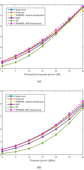
In this subsection, we evaluate the performance of the BNN for the sum rate maximization problem P3 based on the proposed hybrid learning under the assumption that K = 4 and N = 4. The ZF beamforming with pk = PmaxK ,∀k and the RZF beamforming with pk = λk = PmaxK ,∀k are introduced as two baseline solutions. Since the performance of the WMMSE algorithm heavily relies on initialization [9, 10], two different initialization methods, the RZF initialization and the random initialization, are considered and the WMMSE algorithm with the RZF initialization is used to generate samples for the supervised learning in the first stage. First, Fig. 10 shows the sum rate performance averaged over 5000 samples in two different cases: the former case in Fig. 10(a) only considers small-scale fading and and the latter case in Fig. 10(b) considers both small-scale fading and large-scale fading. It is shown that the sum rate performance of all solutions increases as the (normalized) transmit power increases and different initialization methods of the WMMSE algorithm have
Normalized transmit power (dB)
0 5 10 15 20 25 30
Sum rate (bits/s/Hz)
0 5 10 15 20 25 30 Supervised Proposed
WMMSE, random initialization RZF ZF WMMSE, RZF initialization (a) Transmit power (dBm) 0 5 10 15 20 25 30
Sum rate (bits/s/Hz)
0 5 10 15 20 25 Supervised Proposed
WMMSE, random initialization RZF
ZF
WMMSE, RZF initialization
(b)
Fig. 10. The sum rate performance averaged over 5000 samples in two different cases: (a) without large-scale fading and (b) with large-scale fading under{K= 4,N= 4}.
a large performance gap. We observe that in both cases the proposed BNN solution based on the hybrid learning always achieves a performance close to that of the WMMSE algorithm with the RZF initialization, while the performance of the supervised learning-based BNN solution is less satisfactory. This is because the second stage of the hybrid learning method aims to maximize the sum rate and its performance is bounded by the global optimal solution to problem P3. But the aim of the BNN solution based on the supervised learning is to achieve as close to the WMMSE solution as possible and its performance is restricted by the WMMSE solution, which is verified in Figs. 10(a) and 10(b).
We further compare the sum rate performance and the computational complexity, in terms of the execution time per sample, of five beamforming solutions in Figs. 11(a) and 11(b), respectively. The iteration number of the WMMSE algorithm is limited to at most 10. We fix the transmit power budget as
Pmax= 30dBm and assume the transmit antenna number is the same as the user number, i.e., N = K. As the number of transmit antennas increases, the sum rate performance of
Transmit antenna number/ user number
2 3 4 5 6 7 8 9 10 11 12
Sum rate (bits/s/Hz)
10 15 20 25 30 35 40 45 50 55 60 Supervised Proposed
WMMSE, random initialization RZF
ZF
WMMSE, RZF initialization
(a)
Transmit antenna number/ user number
2 3 4 5 6 7 8 9 10 11 12
Execution time per sample (s)
10-5 10-4 10-3 10-2 10-1 100 Supervised Proposed WMMSE RZF ZF (b)
Fig. 11. Comparison of five different beamforming solutions, i.e., the WMMSE solution, BNN solutions based on the supervised learning and the proposed hybrid learning, respectively, the RZF beamforming, and the ZF beamforming: (a) sum rate performance and (b) execution time per sample averaged over 5000 samples under{K=N,Pmax= 30dBm}.
all five solutions increases simultaneously. The performance of the proposed BNN solution based on the hybrid learning method is always close to that of the WMMSE algorithm with the RZF initialization, but is superior to those of the other four solutions and the performance gap becomes larger when the number of the transmit antenna increases. According to Fig. 11(b), the execution time per sample of the BNN solutions based on the supervised learning and hybrid learning methods is at the same level, which is slightly longer than that of the ZF beamforming and the RZF beamforming, for the same reason of Fig. 9(b). As expected, the WMMSE algorithm consumes the most time because of its iterative process. Similar to the other proposed BNNs, it proves that the proposed BNN solution to the sum rate problemP3provides a good balance between the performance and computational complexity.
VIII. CONCLUSIONS
In this paper, we proposed a DL-based framework for fast optimization of the beamforming vectors in the MISO down-link and then devised three BNNs under this framework for the SINR balancing problem under a total power constraint, the power minimization problem under individual QoS constraints, and the sum rate maximization problem under a total power constraint, respectively. The proposed BNNs are based on the CNN structure and expert knowledge. The supervised learning method was adopted for the SINR balancing problem and the power minimization problem because effective algorithms are available for generating training samples. However, there is no practically useful algorithm to find the optimal solution to the nonconvex sum rate maximization problem, therefore the corresponding BNN adoptes a hybrid learning method which first pre-trains the neural network based on the supervised learning method, and then updates the network parameters with the unsupervised learning method to further improve learning performance. Furthermore, in order to reduce the complexity of prediction, the proposed BNNs take advantage of expert knowledge to extract key features instead of predict-ing beamformpredict-ing matrix directly. Simulation results demon-strated that the proposed BNN solutions provided a good balance between the performance and complexity, compared to the existing algorithms.
This work is an attempt to apply the DL technique to beamforming optimization. Actually, a lot of extension works are worth further study. For example, it is unclear so far which input format, I/Q transformation or P/M transformation, is better. In addition, the joint optimization of user selection and beamforming design for the power minimization problem is interesting and it deserves more investigation. Besides, user mobility, machine-type communications, imperfect CSI, fea-sibility detection, and multi-cell scenarios are also interesting extensions for future works.
REFERENCES
[1] W. Xia, G. Zheng, Y. Zhu, J. Zhang, J. Wang, and A. Petropulu, “Deep learning based beamforming neural networks in downlink MISO systems,” inProc. IEEE Int. Conf. Commun. (ICC) Workshop, Shanghai, China, May 2019, pp. 1–5.
[2] E. Bj¨ornson, M. Bengtsson, and B. Ottersten, “Optimal multiuser trans-mit beamforming: A difficult problem with a simple solution structure,” IEEE Signal Process. Mag., vol. 31, no. 4, pp. 142–148, Jul. 2014. [3] H. Boche and M. Schubert, “A general duality theory for uplink and
downlink beamforming,” inProc. IEEE Conf. Veh. Technol. Conf. (VTC), vol. 1, Vancouver, Canada, Sep. 2002, pp. 87–91.
[4] D. Gerlach and A. Paulraj, “Base station transmitting antenna arrays for multipath environments,”Signal Process., vol. 54, no. 1, pp. 59–73, Oct. 1996.
[5] Q. Shi, M. Razaviyayn, M. Hong, and Z. Luo, “SINR constrained beamforming for a MIMO multi-user downlink system: Algorithms and convergence analysis,”IEEE Trans. Signal Process., vol. 64, no. 11, pp. 2920–2933, Jun. 2016.
[6] F. Rashid-Farrokhi, K. R. Liu, and L. Tassiulas, “Transmit beamforming and power control for cellular wireless systems,” IEEE J. Sel. Areas Commun., vol. 16, no. 8, pp. 1437–1450, Oct. 1998.
[7] A. B. Gershman, N. D. Sidiropoulos, S. Shahbazpanahi, M. Bengtsson, and B. Ottersten, “Convex optimization-based beamforming,” IEEE Signal Process. Mag., vol. 27, no. 3, pp. 62–75, May 2010.
[8] A. Wiesel, Y. C. Eldar, and S. Shamai, “Linear precoding via conic optimization for fixed MIMO receivers,”IEEE Trans. Signal Process., vol. 54, no. 1, pp. 161–176, Jan. 2006.