The Effects of Surface Gravity Waves on High-Frequency Acoustic Propagation in Shallow Water

The Effects of Surface Gravity Waves on

High-Frequency Acoustic Propagation

in Shallow Water

Entin A. Karjadi, Mohsen Badiey

, Member, IEEE

, James T. Kirby, and Cihan Bay

ı

nd

ı

r

, Student Member, IEEE

Abstract—A realistic 2-D time-evolving ocean surface model has been combined with an existing acoustic ray-based model to sim-ulate the effects of sea surface roughness on acoustic wave propa-gation in coastal regions. Rough sea surface realizations are gen-erated and used as sea surface boundaries in the acoustic model. An approach to achieve high resolution and accurate results while maintaining computational efficiency of a ray-based model is ap-plied. The results are then compared against a unique set of ex-perimental data collected in 15-m water depth in Delaware Bay. These data include simultaneous environment and acoustic propa-gation (1–18 kHz) measurements. Modeled arrival time-anglefl uc-tuations compare well with data and suggest that there are physical processes which need to be included to improve the model, such as bubbles and turbulence as well as 3-D scattering effects.

Index Terms—Acoustic propagation, acoustic scattering, sea sur-face waves, shallow water.

I. INTRODUCTION

T

in-fluence acoustic wave propagation in the ocean, such as water temperature, salinity, as well as sea bottom and surface conditions. Understanding the impact of each individual param-eter on the acoustic wave propagation is a necessary step in both determining performance level of underwater acoustic commu-nications and developing techniques for using acoustic signals to predict physical parameters in the ocean.

Surface waves are among several environmental parameters that can have apparent influence on underwater acoustic propa-gation. When an acoustic wave interacts with rough sea surface, acoustic wave scattering will occur. This scattered soundfield consists of coherent and incoherent components. In acoustic wave scattering theory, the scale of ocean surface roughness is

Manuscript received August 03, 2010; revised June 20, 2011; accepted September 09, 2011. This work was supported by the U.S. Office of Naval Research (ONR) under Grant N00014-10-1-0396 and in part by the University of Delaware Sea Grant.

Associate Editor: J. F. Lynch.

E. A. Karjadi and M. Badiey are with the College of Earth, Ocean, and Environment, University of Delaware, Newark, DE 19716 USA (e-mail: [email protected]; [email protected]).

J. T. Kirby is with the Center for Applied Coastal Research, University of Delaware, Newark, DE 19716 USA (e-mail: [email protected]).

C. Bayındır is with the Department of Civil and Environmental Engineering, Georgia Institute of Technology, Atlanta, GA 30332 USA (e-mail: [email protected]).

Color versions of one or more of thefigures in this paper are available online at http://ieeexplore.ieee.org.

Digital Object Identifier 10.1109/JOE.2011.2168670

usually specified by the surface roughness (Rayleigh) param-eter which is defined by [1], where is the acoustic wave number, is the root-mean-square displace-ment of ocean surface from its mean level, and is the acoustic grazing angle. In the case where , the surface roughness is small scale and the main part of the scattered energy propa-gates in the specular direction as a coherent wave with inten-sity equals to the product , where is mean scattered pressure. For large sea surface roughness , the coherent component is close to zero and the scatteredfield is almost com-pletely incoherent [1].

Various studies have examined the effects of sea surface roughness. Early works on scattering at rough sea surface were discussed in a literature survey carried out by Fortuin [2]. Two widely known theoretical methods for calculating acoustic scattering from rough surfaces are the Rayleigh–Rice and Kirchhoff approximations [3], [4]. Each approach ap-plies to acoustic scattering from rough surfaces of different scale. Rayleigh–Rice method is based on the small roughness perturbation approximation and is limited by roughness with small heights and slopes. The Kirchhoff method is based on the physical optics approximation and is limited to “gently undulating” surfaces or smooth roughness (although large).

McDaniel and McCammon [5] combined both methods to model scattering from a multiscale rough sea surface. They used the root-mean-square (rms) surface heights and slopes predicted by an empirical surface wave model as parameters for calcu-lating the intensity of acoustic forward scatter. Thorsos [6] also took the approach of using an empirical surface wave model to examine the accuracy and validity of the Rayleigh–Rice and Kirchhoff approximations for low-frequency acoustic scattering from sea surfaces through comparison with exact integral equa-tion results. Instead of only using surface wave statistics such as rms wave heights and slopes, the model used actual rough surface realizations as inputs. Dahl [7] conducted two experi-ments to observe the time and angle characteristics of high-fre-quency sound which was scattered from rough sea surface. The Kirchhoff approximation method was then used to interpret the results and to obtain simple relationships between geometry of acoustical scattering, surface wave conditions, and time-angle spreading of the received signals.

Acoustic propagation models consist of two separate classes: 1) full wave models and 2) ray-based models. When the pro-cessing speed is essential, ray-based models are common choice for modeling acoustic propagation [8]. A coupled 1-D empirical surface model with an acoustic Gaussian beam tracing model

Bellhop [9] was developed [10], [11]. In that study, surface realizations were uncorrelated since for each run of Bellhop, different random realizations of the surface were generated. A Monte Carlo procedure was used to calculate the standard de-viation of arrival time and arrival angle. In comparison, the present study combines the acoustic model Bellhop with a re-alistic, time-evolving sea surface model [12], [13] to simulate thefluctuations of arrival times and arrival angles observed in shallow-water acoustic transmissions. This 2-D approach does not directly address the out-of-plane scattering caused by sur-face waves; to properly model these out-of-plane scattering ef-fects, a full 3-D acoustic wave model may be required. Instead, the present 2-D acoustic model provides a simple and compu-tationally efficient technique of examining thefluctuations of arrival times and angles caused by surface waves.

A High-Frequency Acoustic Experiment (HFA97) was con-ducted on September 22–29, 1997 in a shallow-water region of the Delaware Bay [14]. During the experiment, acoustic signals were transmitted between source–receiver tripods deployed on the seafloor, while highly calibrated environmental data were collected simultaneously at a nearby oceanographic observation platform [15]. Source–receiver tripods were carefully spaced in range so rays with a single surface interaction were easily dis-tinguished in received signals. Extensive analysis of the single surface reflected portion of received signals shows correlation between signalfluctuations and wind speed [14] providing in-formation on the relationship between acoustic transmissions and sea surface variability. The HFA97 data set is used to guide model development and to validate the results.

The focus of this paper is to present a combined water wave and acoustic wave model to predict acoustic signal temporal

fluctuations induced by a sea surface boundary. Comparisons between this simple model output and experimental observa-tions are presented to show the feasibility of the approach and indicate the range of model validity. In Section II, a brief de-scription of the experimental data and some observations are presented. In Section III, the selected acoustic and ocean surface models are introduced along with a description of how the two models are integrated. An approach used in this study to achieve high resolution and more accurate results while maintaining computational efficiency of a ray-based model is discussed in this section. The effect of sea surface resolution on the accuracy of the results is also discussed in this section. Section IV shows comparisons between model output and experimental observa-tions. In Section V, some brief concluding remarks are made along with suggestions for future work.

II. EXPERIMENTALDATA

The HFA97 experiment was conducted in a central region of the Delaware Bay at 75 11 W and 39 01 N. Two bottom mounted tripods, each having an acoustic source and three receiving hydrophones, were placed in 15 m of water depth and separated by 387 m. On each tripod, the source was located 3.125 m above the seafloor and the three receiving hydrophones were located at 0.33, 1.33, and 2.18 m above the seafloor, re-spectively (see Fig. 1). The sources transmitted reciprocal broadband chirp signals over the frequency range of 1–18 kHz.

Fig. 1. HFA97 experiment setup. There are two types of signals observed in the data, those resulting from overhead transmission (dashed lines above tripod A) and those resulting from remote transmission (solid lines between tripods A and B). Group I consists of direct and bottom reflected rays. Group II consists of SSR rays number 2 to number 5.

Fig. 2. Overhead transmission arrival time versus geotime for a 40-s transmis-sion period: (a) during low wind speed ( m/s) and (b) during high wind speed (13.9 m/s). In (b) up and downfluctuations of arrival time across 40-s period indicate surface heightfluctuations.

During the experiment, two different pulse transmission rates were used so as to capture the slow and fast temporal varia-tions of the acousticfield driven by different physical ocean pro-cesses. In thefirst case, a broadband chirp signal was transmitted every 0.345 s for a 5-s duration and repeated every 10 min for the entire experiment which lasted about a week. In the second case, the same chirp signal was transmitted every 0.345 s for a 40-s duration and then repeated every hour for the entire experi-ment. In both sampling cases, each received signal has sufficient time to clear from any scattered signals before the next signal arrives so that overlapping does not occur. In this paper, indi-vidual 0.345-s transmissions are referred to as pings.

For this particular study, analysis focuses on two types of received signals. Thefirst type are those received on thefirst tripod’s highest hydrophone (i.e., 2.18 m above the seafloor) re-sulting from signals transmitted from the source on the same

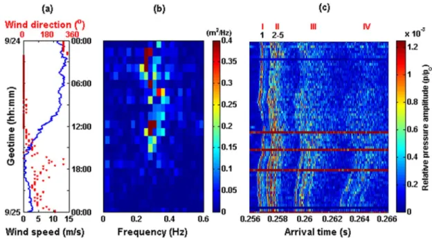
Fig. 3. Surface wave spectra and received acoustic signals arrival time from September 24, 1997 at 00:00:00 L to September 25, 1997 at 00:00:00 L. (a) Wind speed and wind direction. (b) Overhead transmission estimation of spectrum. (c) Signal amplitude versus arrival time for geotimes separated by 10-min intervals. Group I consists of direct and bottom reflected rays. Group II consists of SSR rays. Group III consists of two-surface-reflected rays. Group IV consists of three-surface-reflected rays.

tripod. These signals are referred to as overhead transmission since they involve acoustic waves that travel from the source up to the sea surface and back down to the tripod after one sea sur-face reflection (path is shown by vertical dashed lines in Fig. 1). Plots of two different 40-s overhead transmissions are shown in Fig. 2 for a calm period [wind speed 1 m/s; Fig. 2(a)] and for a rough period [wind speed of 13.9 m/s; Fig. 2(b)]. In Fig. 2(b),

fluctuations in arrival time indicate surface heightfluctuations caused by wind generated surface waves.

The second type of received signals observed in HFA97 data result from acoustic waves traveling from the source on one tripod to the three remotely mounted hydrophone receivers, lo-cated 387 m away on the opposite tripod (paths are shown by solid lines from tripod A to tripod B in Fig. 1). These are referred to as remotely received signals. Group I consists of direct and single bottom reflected paths while Group II consists of single surface reflected (SSR) ray paths. Ray number 2 is surface only bounce, number 3 is bottom-surface bounce, number 4 is sur-face–bottom bounce, and number 5 is bottom–sursur-face–bottom bounce. For these signals, the HFA97 experimental design al-lowed for examination of the time evolution of individual ray paths of SSR rays. This paper focuses on ray number 2 only.

Although no direct surface wave measurements were taken during the HFA97 experiment, overhead transmission signals received on thefirst tripod’s highest hydrophone can be used to obtain information about sea surface fluctuations. Average sea surface height and sound-speed measurements were used to convert arrival time of single surface reflected overhead sig-nals (example in Fig. 2) to surfacefluctuations. For each 40-s transmission time, individual pings were used to estimate sea surface heights at 0.345-s interval. The resulting 40-s time se-ries of the sea surface heights were used to calculate the surface wave frequency spectrum at different 40-s transmission

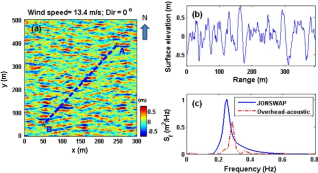
geo-times. Fig. 3 shows the sea surface frequency spectra calculated using the acoustic overhead method described above together with the measured wind speed and direction for a 24-h period from September 24, 1997 at 00:00:00 L to September 25, 1997 at 00:00:00 L. Thefigure shows that spectral level increases with wind speed. Example of comparison with the JOint North Sea WAve Project (JONSWAP) [16] spectrum for wind speed of 13.4 m/s is given in Fig. 5(c).

In this experiment, typically when the wind speed is 10 m/s, the rms surface heights obtained from acoustic overhead trans-missions are smaller than those predicted by the JONSWAP spectra. This is consistent with a more elaborate study of wave prediction using the Simulating WAves Nearshore (SWAN) [17] model, which also gives surface height estimates that greatly exceed the acoustical estimates at higher wind speeds [18]. We suspect that the dropoff in the acoustical estimates versus estab-lished model estimates is due to obscuring of the surface return due to bubbles in the water column after the onset of white-capping, but more efforts on comparing the acoustic overhead method with real ocean wave measurements are required to de-termine its accuracy.

Fig. 3 also shows the arrival time of received acoustic sig-nals for four groups of arrival. In addition to Groups I and II mentioned above, Group III consists of rays with two surface reflections and Group IV consists of rays with three surface

re-flections. During low wind speeds, the signals are distinct and stable while at higher wind speeds the rays break up into smaller peaks resulting from the generation of micro multipaths.

In previous HFA97 analysis, remotely received signals across the three hydrophones were used with a beamforming technique to calculate signal arrival angle as a function of arrival time [14]. By considering the geometry of the HFA97 experimental setup (Fig. 1), the resulting beamformed plots can be used to

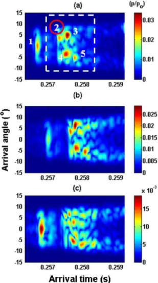
Fig. 4. Remotely received signal arrival angle versus arrival time for calm (wind speed 2 m/s), intermediate (wind speed 5 m/s), and rough (wind speed 13 m/s) periods. For calm period SSR ray paths are easily distinguished in the signal (numbers correspond to ray paths labeled in Fig. 1). The ray paths become more difficult to distinguish for more rough conditions.

distinguish the portion of the received signal corresponding to SSR ray paths (Fig. 4). For calm surface condition ray paths are easily distinguished in the signal (numbers correspond to ray paths labeled in Fig. 1), then they become more difficult to distinguish for rougher conditions.

Since this experiment was aimed at measuring cause and ef-fect between the ocean environment and acoustic propagation, several oceanographic and meteorological measurements were made simultaneously with acoustic measurements. Oceano-graphic measurements included tide height, current, tempera-ture, and salinity profiles while meteorological measurements included air temperature, wind speed, and wind direction. For this study, wind speed and direction measurements will be used to construct the initial sea surface wavefields.

III. MODELINGMETHODS

A. Ray Theory and Gaussian Beam Tracing

Acoustic ray methods are attractive for high-frequency mod-eling problems because they are very much less computationally

intensive compared to full-wave acoustic models while still pro-viding satisfying results. The conventional ray modeling imple-mentations have shortcomings (two common ray tracing anom-alies happen where the shadow zones and caustics occur). To overcome these, there have been a number of efforts proposed to improve the results but retain computational efficiency. One such method is Gaussian beam tracing [9]. With this technique a fan of rays is traced from a point source with trajectories gov-erned by the standard ray equations. The Gaussian beam method associates with each ray a beam with a Gaussian intensity profile normal to the ray. An additional set of equations which governs beam width and curvature is integrated along with the standard ray equations.

The Gaussian beam tracing method has been adapted to the typical ocean acoustics waveguide and has been implemented as a tool called Bellhop [9]. This model has been rigorously tested and the results show excellent agreement with certain full wave models at high frequencies [19]. The method very much mitigates the numerical artifacts affecting standard ray models and still retains the computational efficiency of a ray-based ap-proach.

B. Ocean Surface Waves

In this study, the surface wave is generated by a 2-D linear time-evolving surface model following the approach given by Dommermuth and Yue [12]. There were no direct measure-ments of sea surface wave spectrum in the HFA97 experiment. Therefore, in this study of a fetch-limited coastal area, the JON-SWAP [16] spectrum is used for construction of initial wave

fields. JONSWAP spectrum provides a relationship between wind speed and fetch length with the frequency spectrum. After the construction of the initial wavefield specified by the JONSWAP spectrum, the wave evolution equations are solved numerically to simulate the surface wave realizations. The cor-responding 1-D cross sections of the 2-D surface realizations in the direction of the acoustic track are then used as sea surface boundaries in Bellhop.

1) JONSWAP Frequency Spectrum: There are a number

of empirically derived surface wave models available in the form of surface wave height frequency spectra. A surface wave frequency spectrum represents the distribution of wave energy across a range of frequencies and describes the total energy transmitted by a wavefield at a given time. Wave spectra are strongly influenced by the wave-producing wind and its temporal/spatial characteristics. The spatial variability of wave spectrum is primarily encapsulated into the effect of fetch which is the length of the sea surface over which the wind blows to generate waves. In coastal regions, the wind acts on a limited fetch. As a result, the sea will not become fully developed and the large-scale or swell components of the waves will be significantly reduced in amplitude.

The JONSWAP spectral model computes a sea surface fre-quency spectrum under fetch-limited conditions as func-tion of wind speed [16]. This model is based on an extensive wave measurement program (Joint North Sea Wave Project) car-ried out in 1968 and 1969 in the North Sea. In this study, the JONSWAP spectrum is used to construct the initial wavefield

for the surface model. The fetch length for Delaware Bay area varies between 13 and 22 km depending on wind directions.

The JONSWAP spectral model takes the form

(1) where is the angular frequency, is the gravitational acceler-ation, and is a peak enhancement factor given by

(2) The parameters and are given as

for , and for , while is a function

of fetch length, and wind speed,

(3) and peak frequency is given as

(4) A wave number spectrum can be obtained from the frequency spectrum considering the energy equality under both curves which leads to

(5) where is the wave number of ocean waves. The relationship between and is given by gravity wave dispersion relation-ship

(6) from which the expression for group velocity can be derived (7)

2) Constructing Initial 2-D Surface Wave Realizations: In a

2-D wavefield, we need to consider directional wave spectra given by

(8) where is the directional spreading function given by [20]

(9) where is the mean wave direction and

otherwise.

(10)

To construct an initial water surface, the directional wave spec-trum needs to be transformed to a wave number

spec-trum , where and are wave number

com-ponents along - and -axes, respectively. Considering energy

equality under surfaces of and leads to

(11) where is the Jacobian of the transformation and is given by (12) The amplitude spectrum for each interval can be ob-tained by energy equality

(13) where and are indexing values from 0 to and , respectively. The amplitude spectrum is then mirrored about and to produce by amplitude spectrum. A phase grid is generated using uniformly random phases with values between 0 and . Complex amplitude is generated in wave number space as

(14) A 2-D initial water surface at each of by grid point can be obtained by taking 2-D Fourier transforms of . The surface partitions and must be selected carefully and will be discussed in Section III-C. An initial surface velocity poten-tial is similarly constructed. Details of the computation can be found in [13].

3) Wave Model: The classical kinematic and dynamic

boundary conditions at the free surface in terms of surface

velocity potential , where ,

are given by [12], [13]

(15)

(16)

where is the horizontal gradient, is time,

is the gravitational acceleration, is atmospheric pressure, is water density, and is water surfacefluctuation from the still water level.

In the case of linear surface waves used in this paper, (15) and (16) reduce to

(17) (18) evaluated at . Starting with initial wavefield and , time stepping in (17) and (18) is accomplished using a fourth-order Runge–Kutta integrator with a constant time step [12].

Fig. 5. Example of sea surface realizations generated by the 2-D time-evolving sea surface model. (a) Snapshot of a 2-D wavefield. Waves come from the North (0 wind direction). (b) Corresponding 1-D cross section of sea surface realizations in the direction of acoustic tracks A to B. (c) JONSWAP frequency spectrum with wind speed 13.4 m/s and fetch length of 22 km used to construct the initial wavefield (solid line) and spectrum obtained from overhead acoustic transmission (dashed line).

In the case of nonlinear surface waves, following Dommer-muth and Yue [12], the nonlinear evolution equations for and are given by (15) and (16) while the surface vertical velocity

is expressed as

(19) where are the eigenfunctions representing the expansion of where is the number of eigenmodes,

and where is the expansion order of wave

steepness.

The numerical method used for solving the evolution equa-tions is a two-step procedure [12]. First, given the initial wave

field and , all spatial derivatives are evaluated in wave number space while nonlinear products are calculated in physical space. Second, time integration is accomplished using a fourth-order Runge–Kutta time integrator. Starting from initial conditions, this two-step procedure is repeated for every time step. Further details of the wave model can be found in [13]. C. Integration of Bellhop and Surface Model

Empirical sea surface models have been combined with acoustic models in past studies of similar nature [5], [6], [21] and field data have been used to guide development of such models. A model which includes out-of-plane scattering has recently been developed and compared with field data [7], [22]–[24]. Their results show that out-of-plane scattering de-pends on the value of grazing angle. For single surface bounce with small grazing angle, the out-of-plane scattering is rela-tively small compared to the in-plane scattering [7], [23], [24]. Accordingly, the 2-D acoustic model discussed in the present

Fig. 6. Sketch of a small ray fan used in the model to achieve higher resolution while maintaining computational efficiency of the ray-based model. The star indicates the specular point. Rays with takeoff angles within insonify , length of surface within several surface wavelengths from the specular point.

paper assumes that the out-of-plane scattering of the acoustic

field is negligible for the surface-only reflected rays.

The modeling approach presented here however is unique in terms of using a realistic surface realization to simulate the effects of rough sea surface with computational efficiency of a ray-based model. The concept behind this combined sea surface/acoustic model is the utilization of a 2-D time-evolving rough ocean surface realization and the Gaussian beam tracing model (i.e., Bellhop). The initial wave field is constructed using HFA97 wind speed measurements and the JONSWAP wave number spectrum. The corresponding evolving 1-D cross section of surface realizations in the direction of the acoustic track are then read into Bellhop as (horizontal range, surface height) points with surface partition width and become the upper boundary over the water column through which beams are traced.

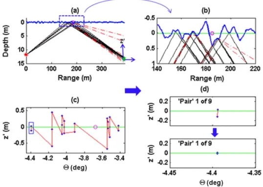
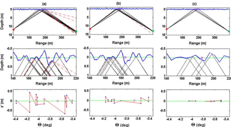
Fig. 7. Example of model run results for wind speed 7 m/s with uniform sound speed over the water column. (a) Eigenrays plot. The stars are source and receiver, and open circle on the water surface is the specular point. is the vertical distance from the receiver and dashed-line rays are those reflected from the surface more than once. (b) Closeup plot near the surface. (c) plot of pair of “eigenrays” versus takeoff angles, where is the vertical distance from the receiver. For real eigenrays, is equal to zero. (d) Midpoint iteration to get the real eigenray whose .

Fig. 5 shows an example of the JONSWAP wave spectrum for constructing the initial wavefield, snapshots of a 2-D wave

field, and the corresponding 1-D cross section of surface realiza-tions. When a beam interacts with the rough surface boundary, the beam trajectory is geometrically reflected from the surface, depending on the surface slope at the point of intersection and the beam’s angle of incidence. The resulting model output sim-ulates thefluctuations in arrival time and arrival angle observed in the HFA97 transmissions.

For the HFA97 case, using the center frequency of the signal (12 kHz), the typical for the Delaware Bay region ( 0.2–0.4 m), and 3.6 , the surface roughness (Rayleigh) parameter , which indicates that the SSR portion of re-ceived signals consists of mostly incoherent scattering (on an ensemble mean basis). This combination of high-frequency and large-scale roughness justifies the approach of geometrically

re-flecting acoustic ray paths from individual points on the rough ocean surface [22].

1) Approach for Higher Resolution and Accuracy: Fig. 6

il-lustrates the approach used in this study to achieve higher res-olution in the model while maintaining computational speed. Since we only consider the single surface-only reflected rays (ray path 2 in Fig. 1), then instead of using a large range of ray takeoff angles to cover a large portion of the surface, we need only to consider a smaller range , which insonifies part of the surface within several surface wavelengths from the specular point. Hence, with the same number of rays, as with larger range of takeoff angle, model resolution is increased while maintaining the same computational time.

For a rough surface, instead of giving eigenrays which go through the receiver, typically Bellhop will give pairs of

“eigen-rays” where the receiver lies between the “eigen“eigen-rays” in the pair. To obtain eigenrays which go through the receiver, we perform a midpoint iteration for each “eigenrays” pair.

Fig. 7 shows an example of model results for a run with random surface realization generated by 7-m/s wind and Delaware Bay average fetch of 10 nautical miles. The sound speed was assumed uniform in depth. Fig. 7(b) is the closeup plot near the surface where the circle is the specular point for

flat surface. Eigenrays shown in dashed lines are those reflected from the surface more than once. We disregard these rays because they usually are much farther away from the receiver. Fig. 7(c) shows values of for the “eigenrays,” where is defined as the vertical distance from the receiver [see Fig. 7(a)]. For real eigenray, is equal to zero. In this particular example, Bellhop gives 9 pairs of “eigenrays” as shown in Fig. 7(c), and a midpoint iteration was performed to obtain the corresponding 9 real eigenrays [Fig. 7(d)].

2) Effects of Sea Surface Resolution: When generating a

sur-face realization, sursur-face partition width must be selected carefully. In previous studies that have involved generating sur-face realization using the spectral method, setting this length has remained an unresolved problem of particular interest [6]. Intu-itively, sea surface with more details will better represent the surface realization, but need to be constructed with a smaller

, and hence at the cost of higher computational time. The model’s results show that the number of “eigenray” pairs increases with the number of surface partition . As an ex-ample, Fig. 8 shows results for a case where the surface was generated by 7-m/s wind resulting in peak period of about 3 s and corresponding wavelength of about 15 m. Here the number of “eigenray” pairs for one instant time step are 9, 7, and 4 for

Fig. 8. Comparisons of model results with different size of surface partitioning . Examples of model run results for wind speed 7 m/s with uniform sound speed over the water column: (a) ( 0.4 m), (b) ( 1.5 m), and (c) ( 6.1 m). Top panels are plots of eigenrays, middle panels are the closeup plots near the surface, and bottom panels are the plots of “eigenray” pairs as output of the model.

, and , respectively, confirming that higher number of is required to capture all the eigenrays. Note that the surface partition of equal to 64 ( 6.1 m) is about one half of the peak wavelength and clearly does not represent the sea surface.

Fig. 9 plots the standard deviation of arrival time as a func-tion of wind speed for different values of where the straight lines represent their linearfits for each . Thisfigure shows that the lines converge for large values of , thus confirming the requirement of using higher resolution of surface partition to obtain higher accuracy. The convergence also confirms that there is an optimal number of surface partition , which relates to computational cost and accuracy.

IV. MODELRESULTS

The results shown hereafter involve the modeling of remotely received signals sent over the distance of 387 m between the two tripods. To assess the accuracy of model results, time-angle

fluctuations of single surface-only reflected beams (ray path 2 in Fig. 1) were measured in the HFA97 data. Time-angle standard deviations for thefirst SSR were calculated for each hourly, 40-s transmission consisting of 115 chirp signals.

Beamformed plots (Fig. 4) were used to pick out the portion of the received signals that correspond to a specific ray path. Fig. 4(a) represents a signal that was transmitted during a calm period (wind speed 2 m/s) and four individual SSR ray paths can be clearly distinguished. In similar plots for rougher periods [Fig. 4(b) and (c)], it becomes more difficult to distinguish be-tween four individual SSR rays due to the breakup and forma-tion of micro multipaths resulting in incoherent scattering at the

Fig. 9. Standard deviation of arrival time as a function of wind speed for dif-ferent sea surface partitioning ( and

).

rough sea surface. For most rough and calm period plots how-ever, it is feasible to pick out the veryfirst arriving SSR ray path in the Group II arrival.

Beamformed results were then used to track time-anglefl uc-tuations of thefirst SSR arrivals in the HFA97 data. Time-angle standard deviations of the first SSR were calculated for the group of 115 signals received during each hourly 40-s trans-mission interval for 19 h from September 24, 1997 at 05:00:00 L to September 25, 1997 at 00:00:00 L. Time-angle standard deviations are then plotted against the wind speed recorded at that transmission time (see Fig. 3). There was significant variation in weather conditions during the HFA97 experiment,

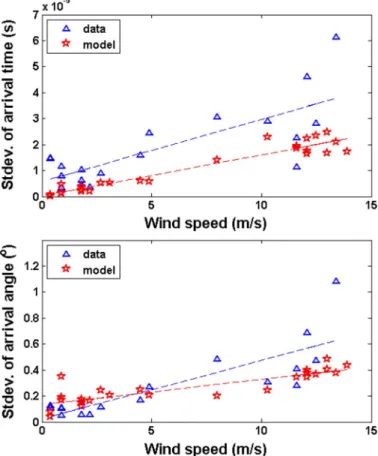
Fig. 10. Model–data comparison of standard deviation of arrival time and ar-rival angle as a function of wind speed. Triangles and stars are data and model results, respectively. Dashed lines are linearfit of the values.

so time-angle standard deviation values are available for a broad range of wind speeds.

Similarly, we ran the model based on 24-h data of wind, tides, and sound-speed profile from September 24, 1997 at 00:00:00 L to September 25, 1997 at 00:00:00 L. At each hour, the sur-face model was run with for 40 s and every 0.345 s the surface realizations were recorded and used as sea surface boundary input to Bellhop. For each realization, a midpoint iter-ation was performed to get the real eigenrays. Then, arrival time for each realization was defined as the minimum arrival time among these eigenrays. As a result, at each hour, there were 115 realizations resulting in 115 arrival times and corresponding ar-rival angles.

To compare model result with data, Fig. 10 plots the stan-dard deviation of arrival time and arrival angle as a function of wind speed for both model and data. Data show that arrival time and arrival anglefluctuations increase as wind speed in-creases, which is also predicted by the model. Notice that there is a large spread in the data, especially during high wind speeds. The model underestimates thefluctuation of arrival time espe-cially during high wind speeds, suggesting that there are phys-ical processes which need to be included in the model, such as bubbles and turbulence effects as well as 3-D or out-of-plane scattering.

V. CONCLUSION

Combining a time-evolving sea surface model and a ray-based acoustic model presents an efficient approach to pre-dictingfluctuations in acoustic signals induced by sea surface roughness. Tracing beams through sea surfacefluctuations and changing beam direction at surface reflection based on surface slope result in a realistic simulation of time-anglefluctuations in received signal. Also, using ray-based acoustic methods makes the model computationally efficient since multiple model runs can be made quickly supporting timely model modification and improvement.

Initial comparisons between this combined model output and HFA97 observations yield good results and suggest that there are other physical processes that need to be included in the model, such as bubble effects. Data from other high-frequency shallow-water acoustic experiments will be compared with the model for further validation of this approach. Also, subsequent work will focus on using this modeling approach to predict am-plitudefluctuations of acoustic signals induced by sea surface roughness. The wave model provides velocity components in the normal direction to the surface, thus calculations of Doppler frequency shift due to sea surface motion can be performed as well. Extending the surface wave model to a nonlinear model to simulate wave breaking and to locate bubbles’ population in the wavefield would appreciably improve the combined acoustic-wave model. Ultimately extending to a 3-D model that includes out-of-plane scattering would be the accurate way to simulate the effects of sea surface roughness on the acoustic propaga-tion.

ACKNOWLEDGMENT

The authors would like to thank all participants of the HFA97 and HFA2000 experiments particularly S. Forsythe, L. Lenain, R. Heitsenrether, and J. Luo for their help in various aspects of the program from 1997 through 2004. They would also like to thank M. Porter for providing help with Bellhop model and for discussions on the project.

REFERENCES

[1] L. Brekhovskikh and Y. Lysanov, Fundamentals of Ocean Acoustics, 3rd ed. New York: Springer-Verlag, 2003, pp. 22–23.

[2] L. Fortuin, “Survey of literature on reflection and scattering of sound waves at the sea surface,”J. Acoust. Soc. Amer., vol. 47, pp. 1209–1228, 1970.

[3] E. I. Thorsos, “The validity of the Kirchhoff approximation for rough surface scattering using a Gaussian roughness spectrum,”J. Acoust. Soc. Amer., vol. 83, pp. 78–92, 1988.

[4] J. A. Ogilvy, Theory of Wave Scattering From Random Rough Sur-faces. London, U.K.: IOP, 1991, ch. 3–4.

[5] S. T. McDaniel and D. F. McCammon, “Composite-roughness theory applied to scattering from fetch limited seas,”J. Acoust. Soc. Amer., vol. 82, pp. 1712–1719, 1987.

[6] E. I. Thorsos, “Acoustic scattering from a ‘Pierson-Moskowitz’ sea surface,”J. Acoust. Soc. Amer., vol. 88, pp. 335–349, 1990. [7] P. H. Dahl, “High-frequency forward scattering from the sea surface:

The characteristic scales of time and angle spreading,”IEEE J. Ocean. Eng., vol. 26, no. 1, pp. 141–151, Jan. 2001.

[8] K. L. Williams, E. I. Thorsos, and W. T. Elam, “Examination of co-herent surface reflection coefficient (CSRC) approximations in shallow water propagation,”J. Acoust. Soc. Amer., vol. 116, pp. 1975–1984, 2004.

[9] M. B. Porter and H. P. Bucker, “Gaussian beam tracing for computing ocean acousticfields,”J. Acoust. Soc. Amer., vol. 82, pp. 1348–1359, 1987.

[10] R. Heitsenrether, “The influence of fetch limited sea surface roughness on high frequency acoustic propagation in shallow water,” M.S. thesis, College Earth Ocean Environ., Univ. Delaware, Newark, DE, 2004. [11] R. Heitsenrether and M. Badiey, “Modeling acoustic signalfluctuations

induced by sea surface roughness,” inProc. High Frequency Ocean Acoust. Conf., La Jolla, CA, 2004, pp. 214–221.

[12] D. G. Dommermuth and D. K. P. Yue, “A high-order spectral method for the study of nonlinear gravity waves,”J. Fluid Mech., vol. 184, pp. 267–288, 1987.

[13] C. Bayindir, “Implementation of a computational model for random di-rectional seas and underwater acoustics,” M.S. thesis, Dept. Civil En-viron. Eng., Univ. Delaware, Newark, DE, 2009.

[14] M. Badiey, Y. Mu, J. A. Simmen, and S. E. Forsythe, “Signal variability in shallow-water sound channels,”IEEE J. Ocean. Eng., vol. 25, no. 4, pp. 492–500, Oct. 2000.

[15] M. Badiey, L. Lenain, K. C. Wong, R. Heitsenrether, and A. Sund-berg, “Long-term acoustic monitoring of environmental parameters in estuaries,” inProc. OCEANS Conf., San Diego, CA, 2003, vol. 1, pp. 366–369.

[16] K. Hasselmann, T. P. Barnett, E. Bouws, H. Carlson, D. E. Cartwright, K. Enke, J. A. Ewing, H. Gienapp, D. E. Haselmann, P. Kruseman, A. Meerburg, P. Muller, D. J. Olbers, K. Richter, W. Sell, and H. Walden, “Measurements of wind-wave growth and swell decay during the Joint North Sea Wave Project (JONSWAP),”Deut. Hydrogr. Inst. Hamburg, vol. 8, pp. 6–95, 1973.

[17] N. Booij, R. C. Ris, and L. H. Holthuijsen, “A third generation wave model for coastal regions 1. Model description and validation,”J. Geo-phys. Res., vol. 104, pp. 7649–7666, 1999.

[18] W. Qin, “Application of the spectral model SWAN in Delaware Bay,” M.S. thesis, Dept. Civil Environ. Eng., Univ. Delaware, Newark, DE, 2005.

[19] M. B. Porter, Acoustic Toolbox [Online]. Available: http://oalib.hlsre-search.com/Rays/index.html

[20] M. A. Donelan, J. Hamilton, and W. H. Hui, “Directional spectra of wind generated waves,”Phil. Trans. Roy. Soc. Lond. A, vol. 315, pp. 509–562, 1985.

[21] M. Siderius and M. B. Porter, “Modeling broadband ocean acoustic transmissions with time-varying sea surface,”J. Acoust. Soc. Amer., vol. 124, pp. 137–150, 2008.

[22] P. H. Dahl, “On the spatial coherence and angular spreading of sound forward scattered from the sea surface: Measurements and interpretive model,”J. Acoust. Soc. Amer., vol. 100, pp. 748–758, 1996. [23] P. H. Dahl, “On bistatic sea surface scattering: Field measurements and

modeling,”J. Acoust. Soc. Amer., vol. 105, pp. 2155–2169, 1999. [24] J. W. Choi and P. H. Dahl, “Measurement and simulation of the channel

intensity impulse response for a site in the east China sea,”J. Acoust. Soc. Amer., vol. 116, pp. 2677–2685, 2006.

Entin A. Karjadireceived the B.S. degree in civil engineering from Bandung Institute of Technology, Bandung, Indonesia, in 1984 and the M.C.E. and Ph.D. degrees in civil engineering from University of Delaware, Newark, in 1991 and 1997, respectively.

She was a faculty member at the Ocean Engi-neering Program, Bandung Institute of Technology, from 1984 to 1986 and from 2001 to 2004. From 1997 to 1999, she was a Postdoctoral Fellow at the Center for Applied Coastal Research, University of Delaware. In 2006, she joined the Ocean Acoustic Laboratory, University of Delaware as a Postdoctoral Researcher. Her research interests are ocean surface wave and acoustic propagation in shallow water.

Mohsen Badiey(M’94) received the Ph.D. degree in applied marine physics and ocean engineering from the Rosenstiel School of Marine and Atmospheric Science, University of Miami, Miami, FL, in 1988.

He was a Postdoctoral Fellow at the Port and Harbour Institute, Ministry of Transport, Tokyo, Japan, from 1988 through 1990, and worked on research problems related to the water–wave interac-tion with seafloor and on seismic wave propagation in continental shelf regions. In 1990, he became a faculty member at the College of Earth, Ocean, and Environment, University of Delaware, Newark, where he presently is a full Professor in the Physical Ocean Science and Engineering Program and in Civil Engineering Department. From 1992 to 1995, he managed the ocean acoustics program at the Office of Naval Research. His research interests are physics of sound and vibration, underwater acoustics in shallow-water regions, acoustical oceanography, underwater acoustic communications, seabed acoustics, and geophysics.

Dr. Badiey is a Fellow of the Acoustical Society of America.

James T. Kirbyreceived the B.Sc. and M.Sc. de-grees in engineering mechanics from Brown Univer-sity, Providence, RI, in 1975 and 1976, respectively, and the Ph.D. in civil engineering from University of Delaware, Newark, in 1983.

He worked as a Research Engineer at Alden Re-search Laboratory, Holden, MA, from 1977 to 1979. He has subsequently been employed with the Ma-rine Sciences Research Center, State University of New York at Stony Brook (1983–1984), Coastal and Oceanographic Engineering Department, University of Florida (1984–1988), and the Civil and Environmental Engineering Depart-ment, University of Delaware (1989-present). He is presently the Edward C. Davis Professor of Civil and Environmental Engineering, and holds a joint ap-pointment in the College of Earth, Ocean, and Environment. His principal re-search areas are ocean surface wave mechanics, near-shore hydrodynamic and sedimentary processes, and tsunamis.

Dr. Kirby is a member of the American Geophysical Union, the American Society of Civil Engineers, and the American Physical Society. He is former Ed-itor-in-Chief of theASCE Journal of Waterway, Port, Coastal and Ocean Engi-neeringand theAGU Journal of Geophysical Research—Oceans. He presently serves on the Board of Governors for the American Institute of Physics.

Cihan Bayındır (S’11) received the B.S. degree, with honors rank, in civil engineering from the Bogaziçi University,ˇ İstanbul, Turkey, in 2007, the M.S. degree in coastal and ocean engineering with a minor in mathematics from the University of Delaware, Newark, in 2009, and the M.S. degree in electrical and computer engineering with minors in mathematics and mechanical engineering from the Georgia Institute of Technology, Atlanta, in 2011, where he is currently working towards the Ph.D. degree at the Department of Civil and Environmental Engineering. He completed his Ph.D. minor studies in electrical and computer engineering with an emphasis on synthetic aperture radar imaging.

He was a Research Assistant for an underwater acoustics project supported by the Office of Naval Research at the University of Delaware. His research inter-ests are synthetic aperture radar and sonar imaging, underwater acoustics,fluid mechanics, computational mathematics, and parallel programming in general.