Propensity score adjusted method for missing data

2013

Propensity score adjusted method for missing data

Minsun Kim Riddles

Iowa State University

Follow this and additional works at:https://lib.dr.iastate.edu/etd Part of theStatistics and Probability Commons

This Dissertation is brought to you for free and open access by the Iowa State University Capstones, Theses and Dissertations at Iowa State University Digital Repository. It has been accepted for inclusion in Graduate Theses and Dissertations by an authorized administrator of Iowa State University Digital Repository. For more information, please [email protected].

Recommended Citation

Riddles, Minsun Kim, "Propensity score adjusted method for missing data" (2013).Graduate Theses and Dissertations. 13287. https://lib.dr.iastate.edu/etd/13287

by

Minsun Kim Riddles

A dissertation submitted to the graduate faculty in partial fulfillment of the requirements for the degree of

DOCTOR OF PHILOSOPHY

Major: Statistics

Program of Study Committee: Jae Kwang Kim, Co-major Professor Sarah M. Nusser, Co-major Professor

Song X. Chen Ranjan Maitra

Cindy L. Yu

Iowa State University Ames, Iowa

2013

DEDICATION

I dedicate this dissertation to God Almighty, who has kept me through the journey of completing this work. I also dedicate this work to my husband, John Riddles, my parents, Soonrim Sim and Namdoo Kim, my sister, Youngsun Kim, my parents-in-law, Deanna and Ron Riddles, and their family, Ronnie, Christine, and Angela Riddles, each of which have been very supportive of me throughout my dissertation.

TABLE OF CONTENTS

DEDICATION . . . ii

ACKNOWLEDGEMENTS . . . v

ABSTRACT . . . vi

CHAPTER 1. INTRODUCTION . . . 1

CHAPTER 2. SOME THEORY FOR PROPENSITY SCORE AD-JUSTMENT ESTIMATORS IN SURVEY SAMPLING . . . 5

2.1 Introduction . . . 6

2.2 Main Results . . . 8

2.3 Augmented propensity score model . . . 14

2.4 Variance estimation . . . 16

2.5 Simulation study . . . 19

2.5.1 Study One . . . 19

2.5.2 Study Two . . . 21

2.6 Conclusion . . . 23

CHAPTER 3. PROPENSITY SCORE ADJUSTMENT METHOD FOR NONIGNORABLE NONRESPONSE . . . 26

3.1 Introduction . . . 27

3.2 Basic setup . . . 29

3.3 Proposed method . . . 33

3.5 Generalized Method of Moment Estimation . . . 39 3.6 Simulation Studies . . . 45 3.6.1 Simulation Study I . . . 45 3.6.2 Simulation Study II . . . 48 3.7 Concluding remarks . . . 53 CHAPTER 4. CONCLUSION . . . 55

APPENDIX A. APPENDIX FOR CHAPTER 3 . . . 57

A.1 Proof of Lemma 3.1. . . 63

A.2 Proof of Theorem 3.1. . . 64

ACKNOWLEDGEMENTS

I would like to express the deepest appreciation to my major professors, Jae-kwang Kim and Sarah Nusser, who continually conveyed encouragement and support in regard to research and scholarship. Without their expertise, guidance, and persistent help, this dissertation would not have been possible. Also, I would like to thank my committee members, Song Chen, Ranjan Maitra, and Cindy Yu, for their feedback on my research. I owe a huge thanks to Graham Kalton, David Mortganstein, and Jill Montaquila at Westat for giving me continuing advice and support. I would also like to thank Reka Howard, Eunice Kim, Jongho Im, Yeunsook Lee, Sixia Chen, and Stephanie Zimmer for being good friends and providing comfort throughout this dissertation.

ABSTRACT

Propensity score adjustment is a popular technique for handling unit nonresponse in sample surveys. When the response probability does not depend on the study variable that is subject to missingness, conditional on the auxiliary variables that are observed throughout the sample, the response mechanism is often called missing at random (MAR) or ignorable, and the propensity score can be computed using the auxiliary variables. On the other hand, if the response probability depends on the study variable that is subject to missingness, the response mechanism is often called not missing at random (NMAR) or nonignorable, and estimating the response probability requires additional distributional assumptions about the study variable. In this dissertation, we investigate the propensity-score-adjustment method and the asymptotic properties of the estimators under two different assumptions, MAR and NMAR.

We discuss some asymptotic properties of propensity-score-adjusted(PSA) estimators and derive optimal estimators based on a regression model for the finite population under MAR. An optimal propensity-score-adjusted estimator can be implemented using an augmented propensity model. Variance estimation is discussed, and the results from two simulation studies are presented. We also consider the NMAR case with an explicit parametric model for response probability and propose a parameter estimation method for the response model that is based on the distributional assumptions of the observed part of the sample instead of making fully parametric assumptions about the population distribution. The proposed method has the advantage that the model for the observed part of the sample can be verified from the data, which leads to an estimator that is less sensitive to model assumptions. Under NMAR, asymptotic properties of PSA estimators

are presented, variance estimation is discussed, and results from two limited simulation studies are presented to compare the performance of the proposed method with the existing methods.

CHAPTER 1.

INTRODUCTION

Throughout the dissertation, we consider a population of three random variables (X, Y, δ) andnindependent realization of the random variables, (xi, yi, δi), i= 1,2,· · · , n.

The auxiliary variable xi is observed for i = 1,2,· · · , n, while yi is observed if and only

if δi = 1, and δi is the response indicator, which is dichotomous, taking values of 1 or 0.

The response mechanism is the distribution of δ, which is crucial in estimation with missing data. The response mechanism is missing completely at random (MCAR) if the response indicator δ is independent of the study variableY, which is subject to missing-ness, and the auxiliary variable X that is observed throughout the sample. A weaker condition for the response mechanism is missing at random (MAR). The response mech-anism is MAR if the response indicator δ is independent of the study variable Y, where Y has missingness, conditional on the auxiliary variable X that is observed throughout the sample [Rubin (1976)]. When the response mechanism is missing at random, the re-sponse mechanism is also called ignorable [Little and Rubin (2002)]. Lastly, the rere-sponse mechanism is not missing at random (NMAR) or nonignorable if the response indicator δ depends on the study variable Y even conditional on the auxiliary variableX.

The parameter of interest is θ0, which is determined by solving E{U(θ;X, Y)} =

0. Under complete response, a consistent estimator of θ0 can be found by solving the

estimating equation,

n

X

i=1

U(θ;xi, yi) = 0. (1.1)

In the presence of missingness, the estimating equation (1.1) cannot be computed. In-stead, one can consider an estimator that is based on the complete cases asPn

0. While the estimation based on the complete cases results in unbiased estimation un-der MCAR, the method results in biased estimation if MCAR does not hold. Also, this method does not utilize the auxiliary variablexi information forδi = 0 cases, which can

be used to improve efficiency.

If the true response probability πi∗ were known, bias could be adjusted by

incor-porating the response probability in the estimating equationPn

i=1δiπ

−1

i∗ U(θ;xi, yi) = 0.

However, the true response probabilities are generally unknown. Instead, we can consider the estimating equation

n

X

i=1

δiπ−i 1U(θ;xi, yi) = 0, (1.2)

where πi = P r(δi = 1|xi, yi) is the conditional response probability. The conditional

response probability πi = P r(δi = 1|xi, yi) is often called the propensity score (PS)

[Rosenbaum and Rubin (1983)].

Since the conditional response probability πi = P r(δi = 1|xi, yi) is also unknown

in general, the conditional response probability still needs to be estimated. One can consider a parametric model for the response probability as πi = π(φ0;xi, yi) for some

φ0 ∈ Ω. Henceforth, this will be referred to as the PS model. If the parameter φ0 can

be estimated consistently by ˆφ, an estimator for θ0 can be found by solving

UP SA(θ; ˆφ) = n

X

i=1

δiπˆ−i 1U(θ;xi, yi) = 0, (1.3)

where ˆπi = π( ˆφ;xi, yi). The estimator that is found by solving (1.3) for θ is called the

propensity-score-adjusted (PSA) estimator.

Before considering the PS model under nonignorable nonresponse, we will first exam-ine the PS adjustment under ignorable nonresponse. Much research has been conducted on the PSA estimator for reducing nonresponse bias under MAR [Fuller et al. (1994); Rizzo et al. (1996)]. Rosenbaum and Rubin (1983) proposed using the PSA approach to estimate the treatment effects in observational studies. Little (1988) reviewed the PSA methods for handling unit nonresponse in survey sampling, Duncan and Stasny (2001)

used the PSA approach to control coverage bias in telephone surveys, Lee (2006) applied the PSA method to a volunteer panel web survey, and Durrant and Skinner (2006) used the PSA approach to address measurement error.

In addition to applications, it is important to understand the asymptotic properties of PSA estimators. Kim and Kim (2007) used a Taylor expansion to obtain the asymptotic mean and variance of PSA estimators and discussed variance estimation. Da Silva and Opsomer (2006) and Da Silva and Opsomer (2009) considered nonparametric methods to obtain PSA estimators and presented their asymptotic properties. Otherwise, despite the popularity of PSA estimators, asymptotic properties of PSA estimators have received little attention in literature.

While much of the existing work on PSA estimators for unit nonresponse assumes that the response mechanism is MAR and the auxiliary variables for the PS model are observed throughout the sample, PSA estimators under nonignorable nonresponse has been receiving more attention in recent research.

As previously mentioned, the response mechanism is crucial in PS estimation since it determines how the parameter in the model for the response probability is estimated. Since, under nonignorable nonresponse, the PS model P r(δi = 1|xi, yi) = π(φ0;xi, yi)

involves yi, which is partially missing, while under ignorable nonresponse, the PS model

P r(δi = 1|xi, yi) = π(φ0;xi) does not involve missing part, estimation under

nonignor-able nonresponse is more complicated than estimation under MAR or ignornonignor-able nonre-sponse. In addition, the methodologies that are developed for ignorable nonresponse cannot be simply applied or extended to estimation under nonignorable nonresponse.

In order to estimate the parameters in the response probability model consistently, assumptions on the distribution of the study variable are added. Fully parametric ap-proaches, which make parametric assumptions on the population distribution of the study variable in additional to the response probability model, are considered in Greenlees et al. (1982), Baker and Laird (1988), and Ibrahim et al. (1999). Parameter estimation without

parametric assumptions on the population distribution of the study variable has been developed in recent works such as Chang and Kott (2008), Kott and Chang (2010), and Wang et al. (2013).

Efficient or optimal estimation of the parameters in the response probability model and inference with the estimated PS model are also addressed. Kim and Kim (2007) showed that the maximum likelihood estimation for the response probability model does not necessarily lead to optimal PSA estimator. Recent works such as Tan (2006) and Cao et al. (2009) also addressed this issue under ignorable nonresponse, but extensions to nonignorable nonresponse model are not well developed.

Our goal is to examine the asymptotic properties of PSA estimators and develop efficient estimation with PS adjustment. Chapter 2 is devoted to PSA estimation under ignorable nonresponse, and Chapter 3 is for PSA estimation under nonignorable nonre-sponse. In Chapter 2, we discuss asymptotic properties of PSA estimators and derive optimal estimators based on a regression model for the finite population under ignorable nonresponse. An optimal PSA estimator is implemented using an augmented propensity model. Variance estimation is discussed, and the results from two simulation studies are presented. In Chapter 3, we propose a new approach that is based on the distribu-tional assumptions of the observed part of the sample instead of making fully parametric assumptions on the overall population distribution and the response mechanism under nonignorable nonresponse. Asymptotic properties of the resulting PSA estimator are presented. Also, to improve the efficiency of the PSA estimator, we incorporate the auxiliary variable X information by using the generalized method of moment. Variance estimation for each estimator is discussed, and results from two limited simulation studies are presented. Concluding remarks are made in Chapter 4.

CHAPTER 2.

SOME THEORY FOR PROPENSITY SCORE

ADJUSTMENT ESTIMATORS IN SURVEY SAMPLING

Published in Survey Methodology, Volume 38, 157-165 Jae Kwang Kim and Minsun Kim Riddles

Abstract

The propensity-scoring-adjustment approach is commonly used to handle selection bias in survey sampling applications, including unit nonresponse and undercoverage. The propensity score is computed using auxiliary variables observed throughout the sample. We discuss some asymptotic properties of propensity-score-adjusted estimators and derive optimal estimators based on a regression model for the finite population. An optimal propensity-score-adjusted estimator can be implemented using an augmented propensity model. Variance estimation is discussed and the results from two simulation studies are presented.

2.1

Introduction

Consider a finite population of size N, where N is known. For each unit i, yi is the

study variable andxi is theq-dimensional vector of auxiliary variables. The parameter of

interest is the finite population mean of the study variable, θ =N−1PN

i=1yi. The finite

population FN ={(x01, y1),(x20, y2),· · · ,(x0N, yN)} is assumed to be a random sample of

size N from a superpopulation distributionF(x, y). Suppose a sample of size n is drawn from the finite population according to a probability sampling design. Let wi = πi−1

be the design weight, where πi is the first-order inclusion probability of unit i obtained

from the probability sampling design. Under complete response, the finite population mean can be estimated by the Horvitz-Thompson (HT) estimator, ˆθHT =N−1

P

i∈Awiyi,

where A is the set of indices appearing in the sample.

In the presence of missing data, the HT estimator ˆθHT cannot be computed. Let r

be the response indicator variable that takes the value one if yis observed and takes the value zero otherwise. Conceptually, as discussed by Fay (1992), Shao and Steel (1999), and Kim and Rao (2009), the response indicator can be extended to the entire population asRN ={r1, r2,· · · , rN}, whereri is a realization of the random variabler. In this case,

the complete-case (CC) estimator ˆθCC =

P

i∈Awiriyi/

P

i∈Awiri converges in probability

to E(Y|r = 1). Unless the response mechanism is missing completely at random in the sense that E(Y|r= 1) =E(Y), the CC estimator is biased. To correct for the bias of the CC estimator, if the response probability

p(x, y) = P r(r= 1|x, y) (2.1) is known, then the weighted CC estimator ˆθW CC = N−1P_i∈Awiriyi/p(xi, yi) can be

used to estimate θ. Note that ˆθW CC is unbiased because

E{X i∈A wiriyi/p(xi, yi)|FN}=E{ N X i=1 riyi/p(xi, yi)|FN}= N X i=1 yi.

If the response probability (2.1) is unknown, one can postulate a parametric model for the response probability p(x, y;φ) indexed by φ ∈Ω such that p(x, y) = p(x, y;φ0)

for some φ0 ∈ Ω. We assume that there exists a

√

n-consistent estimator ˆφ of φ0 such

that

√

nφˆ−φ0

=Op(1), (2.2)

where gn = Op(1) indicates gn is bounded in probability. Using ˆφ, we can obtain the

estimated response probability by ˆpi =p(xi, yi; ˆφ), which is often called the propensity

score Rosenbaum and Rubin (1983). The propensity-score-adjusted (PSA) estimator can be constructed as ˆ θP SA= 1 N X i∈A wi ri ˆ pi yi. (2.3)

The PSA estimator (2.3) is widely used. Many surveys use the PSA estimator to reduce nonresponse bias [Fuller et al. (1994); Rizzo et al. (1996)]. Rosenbaum and Rubin (1983) and Rosenbaum (1987) proposed using the PSA approach to estimate the treatment effects in observational studies. Little (1988) reviewed the PSA methods for handling unit nonresponse in survey sampling. Duncan and Stasny (2001) used the PSA approach to control coverage bias in telephone surveys. Folsom (1991) and Iannacchione et al. (1991) used a logistic regression model for the response probability estimation. Lee (2006) applied the PSA method to a volunteer panel web survey. Durrant and Skinner (2006) used the PSA approach to address measurement error.

Despite the popularity of PSA estimators, asymptotic properties of PSA estimators have not received much attention in survey sampling literature. Kim and Kim (2007) used a Taylor expansion to obtain the asymptotic mean and variance of PSA estimators and discussed variance estimation. Da Silva and Opsomer (2006) and Da Silva and Opsomer (2009) considered nonparametric methods to obtain PSA estimators.

In this paper, we discuss optimal PSA estimators in the class of PSA estimators of the form (2.3) that use a √n-consistent estimator ˆφ. Such estimators are asymptotically unbiased for θ. Finding minimum variance PSA estimators among this particular class of PSA estimators is a topic of major interest in this paper.

Section 2.2 presents the main results. An optimal PSA estimator using an augmented propensity score model is proposed in Section 2.3. In Section 2.4, variance estimation of the proposed estimator is discussed. Results from two simulation studies can be found in Section 2.5 and concluding remarks are made in Section 2.6.

2.2

Main Results

In this section, we discuss some asymptotic properties of PSA estimators. We assume that the response mechanism does not depend on y. Thus, we assume that

P r(r= 1|x, y) = P r(r= 1|x) =p(x;φ0) (2.4)

for some unknown vector φ0. The first equality implies that the data are

missing-at-random (MAR), as we always observe x in the sample. Note that the MAR condition is assumed in the population model. In the second equality, we further assume that the response mechanism is known up to an unknown parameterφ0. The response mechanism

is slightly different from that of Kim and Kim (2007), where the response mechanism is assumed to be under the classical two-phase sampling setup and depends on the realized sample:

P r(r = 1|x, y, I = 1) =P r(r = 1|x, I = 1) =p(x;φ0_A). (2.5) Here, I is the sampling indicator function defined throughout the population. That is, Ii = 1 ifi∈AandIi = 0 otherwise. Unless the sampling design is non-informative in the

sense that the sample selection probabilities are correlated with the response indicator even after conditioning on auxiliary variables Pfeffermann and Sverchkov (1999), the two response mechanisms, (2.4) and (2.5), are different. In survey sampling, assumption (2.4) is more appropriate because an individual’s decision on whether or not to respond to a survey is at his or her own discretion. Here, the response indicator variable ri is

We consider a class of √n-consistent estimators of φ0 in (2.4). In particular, we

consider a class of estimators which can be written as a solution to ˆ

Uh(φ)≡

X

i∈A

wi{ri−pi(φ)}hi(φ) = 0, (2.6)

where pi(φ) = p(xi;φ) for some function hi(φ) = h(xi;φ), a smooth function of xi

and parameter φ. Thus, the solution to (2.6) can be written as ˆφh, which depends

on the choice of hi(φ). Any solution ˆφh to (2.6) is consistent for φ0 in (2.4) because

E{Uˆh(φ0)|FN} = E

h PN

i=1{ri−pi(φ0)}hi(φ0)|FN

i

is zero under the response mecha-nism in (2.4). If we drop the sampling weights wi in (2.6), the estimated parameter ˆφh

is consistent for φ0_A in (2.5) and the resulting PSA estimator is consistent only when the sampling design is non-informative. The PSA estimators obtained from (2.6) using the sampling weights are consistent regardless of whether the sampling design is non-informative or not. According to Chamberlain (1987), any √n-consistent estimator of φ0 in (2.4) can be written as a solution to (2.6). Thus, the choice of hi(φ) in (2.6)

determines the efficiency of the resulting PSA estimator.

Let ˆθP SA,hbe the PSA estimator in (2.3) using ˆpi =pi( ˆφh) with ˆφh being the solution

to (2.6). To discuss the asymptotic properties of ˆθP SA,h, assume a sequence of finite

populations and samples, as in Isaki and Fuller (1982), such thatP

i∈Awiui−

PN

i=1ui =

Op n−1/2N

for any population characteristics ui with bounded fourth moments. We

also assume that the sampling weights are uniformly bounded. That is, K1 < N−1nwi <

K2 for alliuniformly inn, whereK1 andK2 are fixed constants. In addition, we assume

the following regularity conditions:

[C1] The response mechanism satisfies (2.4), where p(x;φ) is continuous in φ with continuous first and second derivatives in an open set containingφ0. The responses

are independent in the sense that Cov(ri, rj|x) = 0 for i 6= j. Also, p(xi;φ) > c

[C2] The solution to (2.6) exists and is unique almost everywhere. The functionhi(φ) =

h(xi;φ) in (2.6) has a bounded fourth moment. Furthermore, the partial derivative

∂{Uˆh(φ)}/∂φ is nonsingular for alln.

[C3] The estimating function ˆUh(φ) in (2.6) converges in probability to Uh(φ) =

PN

i=1{ri−pi(φ)}hi(φ) uniformly inφ. Furthermore, the partial derivative∂{Uˆh(φ)}/∂φ

converges in probability to ∂{Uh(φ)}/∂φ uniformly in φ. The solution φN to

Uh(φ) = 0satisfies N1/2(φN −φ0) = Op(1) under the response mechanism.

Condition [C1] states the regularity conditions for the response mechanism. Condition [C2] is the regularity condition for the solution ˆφh to (2.6). In Condition [C3], some

regularity conditions are imposed on the estimating function ˆUh(φ) itself. By [C2] and

[C3], we can establish the √n-consistency (2.2) of ˆφh.

Now, the following theorem deals with some asymptotic properties of the PSA esti-mator ˆθP SA,h.

Theorem 2.1. If conditions [C1]-[C4] hold, then under the joint distribution of the sampling mechanism and the response mechanism, the PSA estimator θˆP SA,h satisfies

√ nθˆP SA,h−θ˜P SA,h =op(1), (2.7) where ˜ θP SA,h= 1 N X i∈A wi pih0iγ ∗ h+ ri pi (yi−pih0iγ ∗ h) , (2.8) γ_h∗ = (PN i=1rizipih 0 i) −1₍PN i=1riziyi), pi = p(xi;φ0), zi = ∂{p −1_(x i;φ0)}/∂φ, and hi =

h(xi;φ0). Moreover, if the finite population is a random sample from a superpopulation

model, then V(˜θP SA,h)≥Vl ≡V(ˆθHT) + 1 N2E ( X i∈A w_i2 1 pi −1 V(Y|xi) ) . (2.9)

The equality in (2.9) holds when φˆh satisfies

X i∈A wi ( ri p(xi; ˆφh) −1 ) E(Y|xi) = 0, (2.10)

where E(Y|xi) is the conditional expectation under the superpopulation model. Proof. Given pi(φ) = p(xi;φ) and hi(φ) = h(xi;φ), define

ˆ θ(φ,γ) = N−1X i∈A wi pi(φ)h0i(φ)γ+ ri pi(φ) {yi−pi(φ)h0i(φ)γ} .

Since ˆφh satisfies (2.6), we have ˆθP SA = ˆθ( ˆφh,γ) for any choice of γ. We now want to

find a particular choice of γ, say γ∗, such that ˆ

θ( ˆφh,γ∗) = ˆθ(φ0,γ∗) +op n−1/2

. (2.11)

As ˆφh converges in probability to φ0, the asymptotic equivalence (2.11) holds if

E ∂ ∂φ ˆ θ(φ,γ∗)|φ=φ0 =0, (2.12)

using the theory of Randles (1982). Condition (2.12) holds if γ∗ = γ_h∗, where γ_h∗ is defined in (2.8). Thus, (2.11) reduces to

ˆ θP SA,h= 1 N X i∈A wi pih0iγ ∗ h+ ri pi (yi−pih0iγ ∗ h) +op(n−1/2), (2.13)

which proves (2.7). The variance of ˜θP SA,h can be derived as

V(˜θP SA,h) = V(ˆθHT) + 1 N2E ( X i∈A w_i2 1 pi −1 (yi−pih0iγ ∗ h) 2 ) = V(ˆθHT) + 1 N2E " X i∈A w_i2 1 pi −1 {yi−E(Y|xi) +E(Y|xi)−pih0iγ ∗ h} 2 # = V(ˆθHT) + 1 N2E ( X i∈A w_i2 1 pi −1 V(Y|xi) ) + 1 N2E " X i∈A w_i2 1 pi −1 {E(Y|xi)−pih0iγ ∗ h} 2 # , (2.14) where the last equality follows because yi is conditionally independent of E(Y|xi) −

pih0iγ

∗

h, conditioning on xi. Since the last term in (2.14) is non-negative, the inequality

in (2.9) is established. Furthermore, ifE(Y|xi) = pih0iαfor someα, then (2.10) holds and

E(γ_h∗|xi) = α, by the definition ofγh∗. Thus,E(Y|xi)−pih0iγh∗ =−pih0i{γh∗−E(γ

∗

h|xi)}=

In (2.9), Vl is the lower bound of the asymptotic variance of PSA estimators of the

form (2.3) satisfying (2.6). Any PSA estimator that has the asymptotic variance Vl in

(2.9) is optimal in the sense that it achieves the lower bound of the asymptotic variance among the class of PSA estimators with ˆφ satisfying (2.2). The asymptotic variance of optimal PSA estimators of θ is equal to Vl in (2.9). The PSA estimator using the

maximum likelihood estimator ofφ0 does not necessarily achieve the lower bound of the

asymptotic variance.

Condition (2.10) provides a way of constructing an optimal PSA estimator. First, we need an assumption for E(Y|x), which is often called the outcome regression model. If the outcome regression model is a linear regression model of the formE(Y|x) =β0+β10x,

an optimal PSA estimator of θ can be obtained by solving X i∈A wi ri pi(φ) (1,xi) = X i∈A wi(1,xi). (2.15)

Condition (2.15) is appealing because it says that the PSA estimator applied to y = a+b0x leads to the original HT estimator. Condition (2.15) is called the calibration condition in survey sampling. The calibration condition applied to x makes full use of the information contained in it if the study variable is well approximated by a linear function ofx. Condition (2.15) was also used in Nevo (2003) and Kott (2006) under the linear regression model.

If we explicitly use a regression model for E(Y|x), it is possible to construct an estimator that has asymptotic variance (2.9) and is not necessarily a PSA estimator. For example, if we assume that

E(Y|x) = m(x;β0) (2.16)

for some function m(x;·) known up to β0, we can use the model (2.16) directly to

construct an optimal estimator of the form ˆ θopt = 1 N X i∈A wi " m(xi; ˆβ) + ri pi( ˆφ) n yi−m(xi; ˆβ) o # , (2.17)

where ˆβis a√n-consistent estimator of β0 in the superpopulation model (2.16) and ˆφis

a √n-consistent estimator of φ0 computed by (2.6). The following theorem shows that

the optimal estimator (2.17) achieves the lower bound in (2.9).

Theorem 2.2. Let the conditions of Theorem 2.1 hold. Assume thatβˆsatisfiesβˆ=β0+

Op(n−1/2). Assume that, in the superpopulation model (2.16), m(x;β) has continuous first-order partial derivatives in an open set containingβ0. Under the joint distribution of

the sampling mechanism, the response mechanism, and the superpopulation model (2.16), the estimator θˆopt in (2.17) satisfies

√ nθˆopt−θ˜∗opt =op(1), where ˜ θ_opt∗ =N−1X i∈A wi m(xi;β0) + ri pi {yi−m(xi;β0)} , pi =pi(φ0), and V(˜θopt∗ ) is equal to Vl in (2.9).

Proof. Define ˆθopt(β,φ) = N−1P_i∈Awi

m(xi;β) +rip−i 1(φ){yi−m(xi;β)}

.Note that ˆ

θopt in (2.17) can be written as ˆθopt = ˆθopt( ˆβ,φˆ). Since

∂ ∂β ˆ θopt(β,φ) = 1 N X i∈A wi ˘ m(xi;β)− ri pi(φ) ˘ m(xi;β) , where ˘m(xi;β) =∂m(xi;β)/∂β, and ∂ ∂φ ˆ θopt(β,φ) = 1 N X i∈A wirizi(φ){yi −m(xi;β)},

where zi(φ) = ∂{pi−1(φ)}/∂φ, we have E[∂{θˆopt(β,φ)}/∂(β,φ)|β = β0,φ = φ0] = 0

and the condition of Randles (1982) is satisfied. Thus, ˆ

θopt( ˆβ,φˆ) = θˆopt(β0,φ0) +op n−1/2

= ˜θ∗_opt+op n−1/2

The (asymptotic) optimality of the estimator in (2.17) is justified under the joint distribution of the response model (2.4) and the superpopulation model (2.16). When both models are correct, ˆθopt is optimal and the choice of ( ˆβ,φˆ) does not affect the

efficiency of the ˆθoptas long as ( ˆβ,φˆ) is

√

n-consistent. Robins et al. (1994) also advocated using ˆθopt in (2.17) under simple random sampling.

Remark 2.1. When the response model is correct and the superpopulation model (2.16) is not necessarily correct, the choice of βˆdoes affect the efficiency of the optimal estimator. Cao et al. (2009) considered optimal estimation when only the response model is correct. Using Taylor linearization, the optimal estimator in (2.17) with φˆ satisfying (2.6) is asymptotically equivalent to ˜ θ(β) =X i∈A wi m(xi;β) + ri pi {yi−m(xi;β)} − ri pi −1 cβ0pihi ,

wherecβ is the probability limit ofˆcβ ={

P

i∈Awirizi( ˆφ)ˆpih0i( ˆφ)}−1

P

i∈Awirizi( ˆφ){yi−m(xi;β)} and zi(φ) =∂{pi−1(φ)}/∂φ. The asymptotic variance is then equal to

V nθ˜(β)o=V θˆHT +E " X i∈A w_i21−pi pi {yi −m(xi;β)−cβ0pihi} 2 # .

Thus, an optimal estimator of β can be computed by finding βˆ that minimizes

Q(β) = X i∈A w_i2ri 1−pˆi ˆ p2 i n yi−m(xi;β)−ˆc0βpˆihi( ˆφ) o2 .

The resulting estimator is design-optimal in the sense that it minimizes the asymptotic variance under the response model.

2.3

Augmented propensity score model

In this section, we consider optimal PSA estimation. Note that the optimal estimator ˆ

θopt in (2.17) is not necessarily written as a PSA estimator form in (2.3). It is in the

PSA estimator form if it satisfies P

i∈Awiripˆ

−1

can construct an optimal PSA estimator by including m(xi; ˆβ) in the model for the

propensity score. Specifically, given ˆmi =m(xi; ˆβ), ˆpi =pi( ˆφ) and ˆhi =hi( ˆφ), where ˆφ

is obtained from (2.6), we augment the response model by

p∗_i( ˆφ,λ)≡ pˆi

ˆ

pi+ (1−pˆi) exp (λ0+λ1mˆi)

, (2.18)

where λ = (λ0, λ1)0 is the Lagrange multiplier which is used to incorporate the

ad-ditional constraint. If (λ0, λ1)0 = 0, then p∗i( ˆφ,λ) = ˆpi. The augmented response

probability p∗_i( ˆφ,λ) always takes values between 0 and 1. The augmented response probability model (2.18) can be derived by minimizing the Kullback-Leibler distance P i∈Awiriqi∗log(q ∗ i/qi), where q∗i = (1 −p ∗ i)/p ∗

i and qi = (1− pˆi)/pˆi, subject to the

constraint P

i∈Awi(ri/p∗i)(1,mˆi) =

P

i∈Awi(1,mˆi).

Using (2.18), the optimal PSA estimator is computed by ˆ θ∗_{P SA}= 1 N X i∈A wi ri p∗_i( ˆφ,λˆ)yi, (2.19) where ˆλ satisfies X i∈A wi ri p∗_i( ˆφ,λˆ)(1,mˆi) = X i∈A wi(1,mˆi). (2.20)

Under the response model (2.4), it can be shown that ˆ θ∗_{P SA}= 1 N X i∈A wi ˆ b0+ ˆb1mˆi + ri ˆ pi yi−ˆb0−ˆb1mˆi +op n−1/2 , where _ˆ b0 ˆ b1 = ( X i∈A wiri 1 ˆ pi −1 1 ˆ mi 1 ˆ mi 0)−1 X i∈A wiri 1 ˆ pi −1 1 ˆ mi yi. (2.21) Furthermore, by the argument for Theorem 2.1, we can establish that

ˆ θ∗_{P SA}= 1 N X i∈A wi b0+b1mˆi+γh02pihi+ ri pi (yi−b0−b1mˆi−γh02pihi) +op n−1/2 ,

where (b0, b1,γh02) is the probability limit of (ˆb0,ˆb1,γˆh02) with ˆ γh2 = ( X i∈A wirizi( ˆφ)ˆpih0i( ˆφ) )−1 X i∈A wirizi( ˆφ)(yi −ˆb0−ˆb1mˆi) (2.22)

and the effect of estimating φ0 in ˆpi =p(xi; ˆφ) can be safely ignored.

Note that, under the response model (2.4), ( ˆφ,λˆ) in (2.19) converges in probability to (φ0,0), where φ0 is the true parameter in (2.4). Thus, the propensity score from

the augmented model converges to the true response probability. Because ˆλ converges to zero in probability, the choice of ˆβ in ˆmi = m(xi; ˆβ) does not play a role for the

asymptotic unbiasedness of the PSA estimator. The asymptotic variances are changed for different choices of ˆβ.

Under the superpopulation model (2.16), ˆb0+ ˆb1mˆi →E(Y|xi) in probability. Thus,

the optimal PSA estimator in (2.19) is asymptotically equivalent to the optimal estimator in (2.17). Incorporating ˆmi into the calibration equation to achieve optimality is close

in spirit to the model-calibration method proposed by Wu and Sitter (2001).

2.4

Variance estimation

We now discuss variance estimation of PSA estimators under the assumed response model. Singh and Folsom (2000) and Kott (2006) discussed variance estimation for certain types of PSA estimators. Kim and Kim (2007) discussed variance estimation when the PSA estimator is computed with the maximum likelihood method.

We consider variance estimation for the PSA estimator of the form (2.3) where ˆpi =

pi( ˆφ) is constructed to satisfy (2.6) for some hi(φ) = h(xi;φ,βˆ), where ˆβ is obtained

using the postulated superpopulation model. Letβ∗ be the probability limit of ˆβ under the response model. Note that β∗ is not necessarily equal to β0 in (2.16) since we are

not assuming that the postulated superpopulation model is correctly specified in this section.

Using the argument for the Taylor linearization (2.13) used in the proof of Theorem 2.1, the PSA estimator satisfies

ˆ θP SA = 1 N X i∈A wiηi(φ0,β∗) +op n−1/2 , (2.23) where ηi(φ,β) =pi(φ)h0i(φ,β)γ ∗ h + ri pi(φ) {yi−pi(φ)h0i(φ,β)γ ∗ h}, (2.24)

hi(φ,β) = h(xi;φ,β) and γh∗ is defined as in (2.8) withhi replaced byhi(φ0,β∗). Since

pi( ˆφ) satisfies (2.6) withhi(φ) =h(xi;φ,βˆ), ˆθP SA=N−1P_i∈Awiηi( ˆφ,βˆ) holds and the

linearization in (2.23) can be expressed asN−1P

i∈Awiηi( ˆφ,βˆ) =N

−1P

i∈Awiηi(φ0,β

∗₎₊

op(n−1/2). Thus, if (xi, yi, ri) are independent and identically distributed (IID), then

ηi(φ0,β∗) are IID even though ηi( ˆφ,βˆ) are not necessarily IID. Becauseηi(φ0,β∗) are

IID, we can apply the standard complete sample method to estimate the variance of ˆ

ηHT = N−1P_i∈Awiηi(φ0,β

∗_{), which is asymptotically equivalent to the variance of}

ˆ

θP SA =N−1P_i∈Awiηi( ˆφ,βˆ). See Kim and Rao (2009).

To derive the variance estimator, we assume that the variance estimator ˆ V =N−2X i∈A X j∈A Ωijgigj

satisfies ˆV /V(ˆgHT|FN) = 1 +op(1) for some Ωij related to the joint inclusion probability,

where ˆgHT = N−1

P

i∈Awigi for any g with a finite second moment and V(gHT|FN) =

N−2PN

i=1

PN

j=1ΩN·ijgigj,, for some ΩN·ij. We also assume that N

X

i=1

|ΩN·ij|=O(n−1N). (2.25)

To obtain the total variance, the reverse framework of Fay (1992), Shao and Steel (1999), and Kim and Rao (2009) is considered. In this framework, the finite population is first divided into two groups, a population of respondents and a population of non-respondents. Given the population, the sample A is selected according to a probability sampling design. Thus, selection of the population respondents from the whole finite

population is treated as the first-phase sampling and the selection of the sample respon-dents from the population responrespon-dents is treated as the second-phase sampling in the reverse framework. The total variance of ˆηHT can be written as

V(ˆηHT|FN) = V1+V2 =E{V(ˆηHT|FN,RN)|FN}+V{E(ˆηHT|FN,RN)|FN}. (2.26)

The conditional variance term V(ˆηHT|FN,RN) in (2.26) can be estimated by

ˆ V1 =N−2 X i∈A X j∈A Ωijηˆiηˆj, (2.27)

where ˆηi =ηi( ˆφ,βˆ) is defined in (2.24) withγh∗ replaced by a consistent estimator such as

ˆ

γ_h∗ ={P

i∈Awirizi( ˆφ)ˆpihˆ0i}

−1P

i∈Awirizi( ˆφ)yi,and ˆhi =h(xi; ˆφ,βˆ). To show that ˆV1 is

also consistent forV1 in (2.26), it suffices to show thatV{n·V(ˆηHT|FN,RN)|FN}=o(1),

which follows by (2.25) and the existence of the fourth moment. See Kim et al. (2006). The second term V2 in (2.26) is

V{E(ˆηHT|FN,RN)|FN} = V N−1 N X i=1 ηi|FN ! = 1 N2 N X i=1 1−pi pi yi−pih∗ 0 i γ ∗ h 2 ,

where h∗_i =h(xi;φ0,β∗). A consistent estimator of V2 can be derived as

ˆ V2 = 1 N2 X i∈A wiri 1−pˆi ˆ p2 i yi−pˆihˆ 0 iγˆ ∗ h 2 , (2.28)

where γ_h∗ is defined after (2.27). Therefore, ˆ

V θˆP SA

= ˆV1 + ˆV2, (2.29)

is consistent for the variance of the PSA estimator defined in (2.3) with ˆpi = pi( ˆφ)

satisfying (2.6), where ˆV1 is in (2.27) and ˆV2 is in (2.28).

Note that the first term of the total variance is V1 = Op(n−1), but the second term

isV2 =Op(N−1). Thus, when the sampling fraction nN−1 is negligible, that is,nN−1 =

variance. Otherwise, the second term V2 should be taken into consideration, so that a

consistent variance estimator can be constructed as in (2.29).

Remark 2.2. The variance estimation of the optimal PSA estimator with augmented propensity model (2.18) with ( ˆφ,λˆ) satisfying (2.20) can be derived by (2.29) using ηˆi =

ˆ_{b0 + ˆb1mˆi+ ˆγ}0

h2pˆihˆi+ripˆi−1(yi−ˆb0−ˆb1mˆi−γˆh02pˆihˆi) where (ˆb0,ˆb1) and γˆh2 are defined

in (2.21) and (2.22), respectively.

2.5

Simulation study

2.5.1 Study One

Two simulation studies were performed to investigate the properties of the proposed method. In the first simulation, we generated a finite population of size N = 10,000 from the following multivariate normal distribution:

  x1 x2 e  ∼N     2 −1 0  ,   1 0.5 0 0.5 1 0 0 0 1    .

The variable of interesty was constructed asy= 1 +x1+e.We also generated response

indicator variables ri independently from a Bernoulli distribution with probability

pi =

exp(2 +x2i)

1 + exp(2 +x2i)

.

From the finite population, we used simple random sampling to select two samples of size, n = 100 and n = 400, respectively. We used B = 5,000 Monte Carlo samples in the simulation. The average response rate was about 69.6%.

To compute the propensity score, a response model of the form p(x;φ) = exp(φ0+φ1x2)

1 + exp(φ0+φ1x2)

(2.30) was postulated and an outcome regression model of the form

was postulated to obtain the optimal PSA estimators. Thus, both models are correctly specified. From each sample, we computed four estimators of θ =N−1PN

i=1yi:

1. (PSA-MLE) : PSA estimator in (2.3) with ˆpi = pi( ˆφ) and ˆφ being the maximum

likelihood estimator of φ.

2. (PSA-CAL) : PSA estimator in (2.3) with ˆpi satisfying the calibration constraint

(2.15) on (1, x2i).

3. (AUG) : Augmented PSA estimator in (2.19). 4. (OPT) : Optimal estimator in (2.17).

In the augmented PSA estimators, ˆφwas computed by the maximum likelihood method. Under model (2.30), the maximum likelihood estimator ofφ= (φ0, φ1)0was computed by

solving (2.6) withhi(φ) = (1, x2i)0. Parameter (β0, β1) for the outcome regression model

was computed using ordinary least squares, regressing y onx1. In addition to the point

estimators, we also computed the variance estimators of the point estimators. The vari-ance estimators of the PSA estimators were computed using the pseudo-values in (2.24) and the hi(φ) corresponding to each estimator. For the augmented PSA estimators, the

pseudo-values were computed by the method in Remark 2.

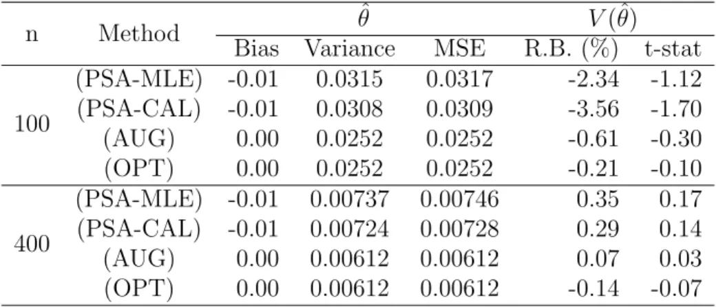
Table 2.1 presents the Monte Carlo biases, variances, and mean square errors of the four point estimators and the Monte Carlo percent relative biases and t-statistics of the variance estimators of the estimators. The percent relative bias of a variance estimator

ˆ

V(ˆθ) is calculated as 100×{VM C(ˆθ)}−1[EM C{Vˆ(ˆθ)}−VM C(ˆθ)], whereEM C(·) andVM C(·)

denote the Monte Carlo expectation and the Monte Carlo variance, respectively. The t-statistic in Table 1 is the test statistic for testing the zero bias of the variance estimator. See Kim (2004).

1. All of the PSA estimators are asymptotically unbiased because the response model (2.30) is correctly specified. The PSA estimator using the calibration method is slightly more efficient than the PSA estimator using the maximum likelihood estimator, because the last term of (2.14) is smaller for the calibration method as the predictor forE(Y|xi) =β0+β1x1i is better approximated by a linear function

of (1, x2i) than by a linear function of (ˆpi,pˆix2i).

2. The augmented PSA estimator is more efficient than the direct PSA estimator (2.3). The augmented PSA estimator is constructed by using the correctly specified regression model (2.31) and so it is asymptotically equivalent to the optimal PSA estimator in (2.17).

3. Variance estimators are all approximately unbiased. There are some modest biases in the variance estimators of the PSA estimators when the sample size is small (n= 100).

2.5.2 Study Two

In the second simulation study, we further investigated the PSA estimators with a non-linear outcome regression model under an unequal probability sampling design. We generated two stratified finite populations of (x, y) with four strata (h = 1,2,3,4), wherexhi were independently generated from a normal distributionN(1,1) andyhiwere

dichotomous variables that take values of 1 or 0 from a Bernoulli distribution with probability p1yhi or p1yhi. Two different probabilities were used for two populations,

respectively :

1. Population 1 (Pop1): p1yhi = 1/{1 + exp(0.5−2x)}

2. Population 2 (Pop2): p2yhi = 1/[1 + exp{0.25(x−1.5)2−1.5}]

In addition to xhi and yhi, the response indicator variables rhi were generated from a

the four strata wereN1 = 1,000, N2 = 2,000, N3 = 3,000,and N4 = 4,000,respectively.

In each of the two sets of finite population, a stratified sample of size n = 400 was independently generated without replacement, where a simple random sample of size nh = 100 was selected from each stratum. We used B = 5,000 Monte Carlo samples in

this simulation. The average response rate was about 67%.

To compute the propensity score, a response model of the form

p(x;φ) = exp (φ0+φ1x) 1 + exp (φ0+φ1x)

was postulated for parameter estimation. To obtain the augmented PSA estimator, a model for the variable of interest of the form

m(x;β) = exp (β0+β1x) 1 + exp (β0+β1x)

(2.32)

was postulated. Thus, model (2.32) is a true model under (Pop1), but it is not a true model under (Pop2).

We computed four estimators:

1. (PSA-MLE): PSA estimator in (2.3) using the maximum likelihood estimator ofφ. 2. (PSA-CAL): PSA estimator in (2.3) with ˆpi satisfying the calibration constraint

(2.15) on (1, x).

3. (AUG-1) : Augmented PSA estimator ˆθ_{P SA}∗ in (2.19) with ˆβ computed by the maximum likelihood method.

4. (AUG-2) : Augmented PSA estimator ˆθ_{P SA}∗ in (2.19) with ˆβ computed by the method of Cao et al. (2009) discussed in Remark 1.

We considered the the augmented PSA estimator in (2.19) with ˆpi =pi( ˆφ), where ˆφ

is the maximum likelihood estimator ofφ. The first augmented PSA estimator (AUG-1) used ˆmi =m(xi; ˆβ) with ˆβfound by solvingP4_h=1P_i∈Ahwhirhi{yhi−m(xhi;β)}(1, xhi) =

0, where Ah is the set of indices appearing in the sample for stratum h and whi is the

sampling weight of unit i for stratum h.

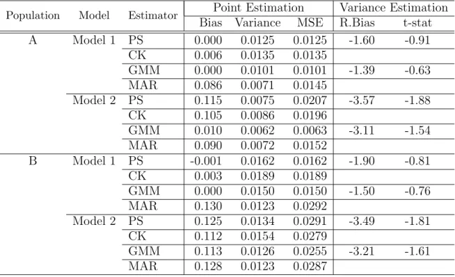
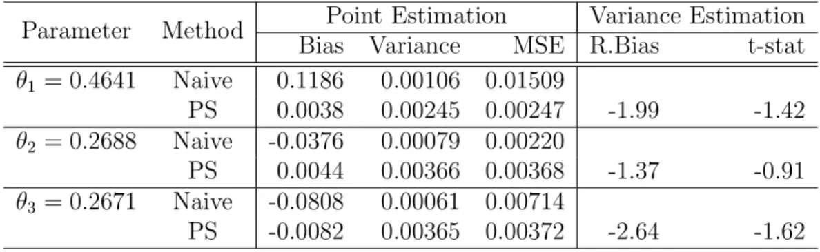
Table 2.2 presents the simulation results for each method. In each population, the augmented PSA estimator shows some improvement comparing to the PSA estimator using the maximum likelihood estimator ofφ or the calibration estimator of φin terms of variance. Under (Pop1), since model (2.32) is true, there is essentially no difference between the augmented PSA estimators using different methods of estimating β. How-ever, under (Pop2), where the assumed outcome regression model (2.32) is incorrect, the augmented PSA estimator with ˆβ computed by the method of Cao et al. (2009) results in slightly better efficiency, which is consistent with the theory in Remark 1. Variance estimates are approximately unbiased in all cases in the simulation study.

2.6

Conclusion

We have considered the problem of estimating the finite population mean of y under nonresponse using the propensity score method. The propensity score is computed from a parametric model for the response probability, and some asymptotic properties of PSA estimators are discussed. In particular, the optimal PSA estimator is derived with an additional assumption for the distribution of y. The propensity score for the optimal PSA estimator can be implemented by the augmented propensity model presented in Section 2.3. The resulting estimator is still consistent even when the assumed outcome regression model fails to hold.

We have restricted our attention to missing-at-random mechanisms in which the response probability depends only on the always-observed x. If the response mechanism also depends on y, PSA estimation becomes more challenging. PSA estimation when missingness is not at random is beyond the scope of this article and will be a topic of future research.

Acknowledgement

The research was partially supported by a Cooperative Agreement between the US Department of Agriculture Natural Resources Conservation Service and Iowa State Uni-versity. The authors wish to thank F. Jay Breidt, three anonymous referees, and the associate editor for their helpful comments.

Table 2.1 Monte Carlo bias, variance and mean square error(MSE) of the four point estimators and percent relative biases (R.B.) and t-statistics(t-stat) of the variance estimators based on 5,000 Monte Carlo samples

n Method θˆ V(ˆθ)

Bias Variance MSE R.B. (%) t-stat

100 (PSA-MLE) -0.01 0.0315 0.0317 -2.34 -1.12 (PSA-CAL) -0.01 0.0308 0.0309 -3.56 -1.70 (AUG) 0.00 0.0252 0.0252 -0.61 -0.30 (OPT) 0.00 0.0252 0.0252 -0.21 -0.10 400 (PSA-MLE) -0.01 0.00737 0.00746 0.35 0.17 (PSA-CAL) -0.01 0.00724 0.00728 0.29 0.14 (AUG) 0.00 0.00612 0.00612 0.07 0.03 (OPT) 0.00 0.00612 0.00612 -0.14 -0.07

Table 2.2. Monte Carlo bias, variance and mean square error of the four point estimators and percent relative biases (R.B.) and t-statistics of the variance estimators, based on 5,000 Monte Carlo samples

Population Method θˆP SA V(ˆθP SA)

Bias Variance MSE R.B. (%) t-stat

Pop1 (PSA-MLE) 0.00 0.000750 0.000762 -1.13 -0.57 (PSA-CAL) 0.00 0.000762 0.000769 -1.45 -0.72 (AUG-1) 0.00 0.000745 0.000757 -1.73 -0.86 (AUG-2) 0.00 0.000745 0.000757 -1.83 -0.91 Pop2 (PSA-MLE) 0.00 0.000824 0.000826 0.29 0.14 (PSA-CAL) 0.00 0.000829 0.000835 -0.94 -0.46 (AUG-1) 0.00 0.000822 0.000823 -0.71 -0.35 (AUG-2) 0.00 0.000820 0.000821 -0.61 -0.30

CHAPTER 3.

PROPENSITY SCORE ADJUSTMENT

METHOD FOR NONIGNORABLE NONRESPONSE

To be submitted to Journal of the American Statistical Association Minsun Kim Riddles and Jae-kwang Kim

Abstract

Propensity score adjustment is a popular technique for handling unit nonresponse in sample surveys. If the response probability depends on the study variable that is subject to missingness, estimating the response probability often relies on additional distributional assumptions about the study variable. Instead of making fully parametric assumptions about the population distribution of the study variable and the response mechanism, we propose a new approach of maximum likelihood estimation that is based on the distributional assumptions of the observed part of the sample. Since the model for the observed part of the sample can be verified from the data, the proposed method is less sensitive to failure of the assumed model of the outcomes. Generalized method of moments can be used to improve the efficiency of the proposed estimator. Variance estimation is discussed and results from two limited simulation studies are presented to compare the performance of the proposed method with the existing methods.

Key words: Exponential tilting model, Nonresponse weighting adjustment, Nonresponse error, Not missing at random

3.1

Introduction

Analysis of survey data involves the assumption that data are collected from a ran-domly selected sample that is representative of the target population. When the repre-sentativeness of the sample at hand is in question, the relationship of the variables in the sample does not necessarily hold in the population. In practice, survey estimates are subject to various forms of selection bias that stems from a systematic difference between the sample and the target population. Sources of selection bias at the unit-level include discrepancies between the sampling frame and the target population, called coverage error, and failure to obtain responses from the full sample, called nonresponse error. Reducing the selection bias is a crucial part of improving the scientific foundation for generalizing survey results to the target population.

Nonresponse error has become a major problem in sample surveys as participation rates have declined in many surveys. Weighting adjustments are commonly used to ad-just for unit nonresponse. Classical approaches include poststratification [Holt and Smith (1979)], regression weighting [Bethlehem (1988)], and raking ratio estimation [Deville et al. (1993)]. Propensity score (PS) weighting, which increases the sampling weights of the respondents using their inverse response probabilities, is a popular approach for handling unit nonresponse. Most of the existing work on PS modeling for unit nonre-sponse assumes an ignorable mechanism for missing data, and the auxiliary variables for the PS model are observed throughout the sample. For examples, see Ekholm and Laaksonen (1991), Fuller et al. (1994), Lindstr¨om and S¨arndal (1999), and Kott (2006). If the missing mechanism is not ignorable, that is, the response mechanism is related to the variable of interest directly or indirectly, then the realized sample may over-represent individuals that are interested in the topic of the survey and survey estimates may be biased [Groves et al. (2004)]. PS modeling with nonignorable nonresponse is challenging because the covariates for the PS model are not always observed.

In this paper, we consider parameter estimation for a PS model under nonignorable nonresponse. In order to estimate the parameters in the PS model consistently, additional assumptions are imposed on the distribution of the study variable that is subject to missingness. A fully parametric approach, which makes parametric assumptions about the population distribution of the study variable can be used to estimate the parameters in the response model, but the estimates can be very sensitive against the failure of the assumed response model. Instead of the fully parametric approach, we consider an alternative modeling approach that uses parametric model assumptions about the study variable in the responding part of the sample. The resulting PS weighed estimator is shown to be consistent under the correct specification of the response probability model. In addition to PS modeling, efficient or optimal estimation of the parameters in the PS model and inference with the estimated PS model are also addressed. The maximum likelihood estimation of the PS model parameters does not necessarily lead to optimal PS estimation [Kim and Kim (2007)]. Recent works such as Tan (2006), Cao et al. (2009), Kim and Riddles (2012) have partially addressed these issues under ignorable response mechanisms, but extension to nonignorable nonresponse model is not well developed. Recent works such as Chang and Kott (2008), Kott and Chang (2010), and Wang et al. (2013) have addressed parameter estimation under nonignorable nonresponse, but the optimality was not discussed. Efficient estimation and valid inferential tools for nonig-norable nonresponse are discussed in Section 3.5. The proposed estimators are directly applicable to the survey sampling setup, as illustrated in Section 3.6.2.

In Section 3.2, the basic setup is introduced. In Section 3.3, an approach to estimating response model parameters is proposed. In Section 3.4, variance estimation is discussed. In Section 3.5, the generalized method of moments is used to incorporate the auxiliary variables that are observed in the sample. Results from two simulation studies are presented in Section 3.6, and concluding remarks are made in Section 3.7.

3.2

Basic setup

Consider an infinite population with three random variables (X, Y, δ). Let (xi, yi),

i = 1,2,· · · , n be n independent realizations of (X, Y) in the population. In addition,

we assume thatδ is dichotomous taking values of 1 or 0, andyi is observed if and only if

δi = 1. The auxiliary variablexi is always observed fori= 1,2,· · · , n. We are interested

in estimatingθ, which is uniquely determined by solving E{U(θ;X, Y)}= 0.

In the presence of missing data, if the true response probability πi were known,

an unbiased consistent estimator of θ, ˆθP S1, could be obtained by solving UP S1(θ) =

Pn

i=1δiπi−1Ui(θ) = 0 for θ,where Ui(θ) =U(θ;xi, yi). However, the true response

prob-abilities are unknown in general and need to be estimated consistently from the sample. On the other hand, ifπi2 =P r(δi = 1 |xi, yi) are known, then the resulting estimator

ˆ θP S2 obtained by solving UP S2(θ) = n X i=1 δi πi2 Ui(θ) = 0 (3.1)

is also unbiased, because E{UP S2(θ)} = E ( _n X i=1 E δiπi−21Ui(θ)|xi, yi ) = E ( _n X i=1 π_i−₂1Ui(θ)E(δi |xi, yi) ) =E ( _n X i=1 Ui(θ) ) .

Thus, we only have to postulate a model for the conditional response probability πi2,

conditional on xi and yi. Furthermore, ˆθP S2 from (3.1) is more efficient than ˆθP S1 using

the true response probability, because ˆθP S2 is essentially the conditional expectation of

ˆ

θP S1 given the observation. See Lemma 1 of Kim and Skinner (2013). Thus, we consider

estimating θ by ˆθP S2 in (3.1).

To compute the PS estimator, ˆθP S2, we assume that x can be decomposed as x =

(x1,x2) and the dimension ofx2 is greater than or equal to one. We consider a parametric

model for the response indicator as follows:

for some function π(·) known up to the response model parameter φ0. The assumed

response model (3.2) implies that the response mechanism is nonignorable in the sense that the response mechanism is not independent of the study variable y even after ad-justing for the auxiliary variablex. The model (3.2) also implies that response indicator does not depend on x2 given x1 and y. Variable x2 is sometimes the called nonresponse

instrumental variable, which means that it does not directly related with the response mechanism but it helps to identify the parameters in the response mechanism. The as-sumption of conditional independence of the response indicator δ and the instrumental variablex2 in (3.2) makes the parameterφ0 in (3.2) identifiable. See Wang et al. (2013)

for details.

Under the parametric assumption (3.2), we now assume that δi are generated from

a Bernoulli distribution with probability πi(φ0) ≡π(x1i, yi;φ0) for some φ0. If yi were

observed throughout the sample, the likelihood function of φwould be L(φ) =

n

Y

i=1

{π(x1i, yi;φ)}δi{1−π(x1i, yi;φ)}(1−δi),

and the maximum likelihood estimator (MLE) ofφcould be obtained by solving the score equation S(φ) =∂logL(φ)/∂φ=0.The score equation S(φ) = 0can be expressed as

S(φ) = n X i=1 s(φ;δi,x1i, yi) = n X i=1 {δi−π(x1i, yi;φ)}z(x1i, yi;φ) = 0, (3.3)

where z(x1i, yi;φ) = ∂logit{π(x1i, yi;φ)}/∂φ, and logit(p) = log{p/(1−p)}. However,

as some of yi are missing, the score equation (3.3) is not applicable. Instead, we can

consider maximizing the observed likelihood function Lobs(φ) = n Y i=1 {π(x1i, yi;φ)} δi Z {1−π(x1i, y;φ)}f(y|xi)dy 1−δi , (3.4) where f(y|x) is the true conditional distribution of y given x.

The MLE of φ can be obtained by solving the observed score equation, Sobs(φ) =

∂logLobs(φ)/∂φ= 0. Finding the solution to the observed score equation is

parameters. Instead of solving the observed score equation, another way to find the MLE of φ is to solve the mean score equation ¯S(φ) = 0, where

¯ S(φ) = n X i=1 ¯si(φ) = n X i=1 E{s(φ;δ,x1, y)|δi,xi, yobs,i} = n X i=1 [δis(φ;δi,x1i, yi) + (1−δi)E0{s(φ;δi,x1i, Y)|xi}],(3.5)

where s(φ;δ,x1, y) is defined in (3.3), yobs,i is yi if δi = 1 and is null if δi = 0, and

E0(· |xi) =E(· |xi, δi = 0). The mean score function (3.5) is the conditional expectation

of the score function given all the observed data (δi,xi, yobs,i), for i = 1,2,· · · , n. The

equivalence of Sobs(φ) and ¯S(φ) is given in Lemma 3.1, which was originally discussed

in Louis (1982).

Lemma 3.1. Under some regularity conditions,

Sobs(φ) = ¯S(φ)

holds, where Sobs(φ) =∂logLobs(φ)/∂φ, Lobs(φ)is defined in (3.4), andS¯(φ) is defined in (3.5).

The proof of Lemma 3.1 is provided in Appendix A.1.

In order to solve the mean score equation ¯S(φ) = 0, the conditional distribution for nonrespondents, f0(y | x) = f(y | x, δ = 0), is needed to compute the conditional

expectation of the score function of nonrespondents. If a parametric model f(y | x) = f(y |x;β) is assumed in addition to (3.2), the conditional expectation for nonrespondents can be derived using two models, f(y | x;β) and P(δ = 1 | x, y;φ), and the maximum likelihood estimate for (β,φ) can be computed jointly, as considered by Greenlees et al. (1982), Baker and Laird (1988), and Ibrahim et al. (1999). The fully parametric approach finds the maximum likelihood estimator that maximizes the following likelihood function

L(β,φ) = n Y i=1 {π(x1i, yi;φ)f(y|x;β)}δi Z {1−π(x1i, y;φ)}f(y|xi;β)dy 1−δi .

However, the fully parametric model approach, which assumes parametric models for both the response mechanism and the conditional distribution f(y| x), is known to be sensitive to the failure of model assumptions [Kenward and Molenberghs (1988)]. Also, it can be challenging to check both models under nonignorable nonresponse. We will consider an alternative approach of computing the MLE of φ in Section 3.3.

Instead of maximum likelihood estimation for the response model parameter φ, one can find a consistent estimator of φby forcing the PS estimator of auxiliary variables to match the complete sample mean of auxiliary variables as follows:

n X i=1 δi πi(φ) xi = n X i=1 xi. (3.6)

Condition (3.6) is often called the calibration condition in survey sampling. Chang and Kott (2008) showed the consistency of the PS estimator satisfying the calibration condi-tion (3.6) under some regularity conditions when the parametric response model (3.2) is correctly specified and there exists a linear relationship between the auxiliary variables

X and the study variable Y. Wang et al. (2013) also proved the asymptotic normality of the PS estimator satisfying (3.6) without assuming the linear models. The proposed method in Chang and Kott (2008) and Wang et al. (2013), which is based on the general-ized method of moments (GMM), find estimates by minimizing{A(θ;φ)}T_W−1_A(θ;φ),

where A(θ;φ) =    Pn i=1{δiπi−1(φ)xi−xi} Pn i=1{δiπ −1 i (φ)yi−θ}   ,

xi isi-th observation of benchmark covariates and W−1 is some weight matrix. By this

method, calibration can correct the nonresponse bias. Here, use ofxi in (3.6) makes the

3.3

Proposed method

In this section, we consider an alternative approach of obtaining the maximum like-lihood estimator of response model parameter φ without specifying the conditional dis-tribution of f(y | x). Note that with the fully parametric approach, the conditional expectation in (3.5) is taken with respect to the conditional distribution,

f(y|x, δ= 0) = f(y|x) P(δ = 0|x, y) E{P(δ= 0 |x, Y)|x}.

If a parametric model for f(y | x) were correctly specified, the MLE of the response model parameter φ could be obtained by solving ¯S(φ) = 0, where ¯S(φ) is defined in (3.5), and the resulting MLE will be consistent and the most efficient in the sense that it achieves the Cramer-Rao lower bound. On the other hand, these attractive features are not guaranteed when the parametric model for f(y | x) is not correctly specified. Besides, finding a correct model is quite challenging when only a part ofy is observed.

We consider an alternative approach that uses a model for the conditional distribution of the study variable ygiven the auxiliary variables xfor respondents, denoted byf1(y|

x) =f(y|x, δ= 1), instead of using a model for the conditional distribution of y given

x, f(y | x). To obtain the conditional distribution of y given x for nonrespondents, denoted byf0(y|x) =f(y|x, δ = 0), from the conditional distribution for respondents,

f1(y|x), the following Bayes formula can be used

f0(y|x) = f1(y |x)

O(x, y)

E{O(x, Y)|x, δ= 1}, (3.7) where O(x, y) =P(δ = 0| x, y)/P(δ = 1| x, y) is the conditional odds of nonresponse. In (3.7), we only need the response model (3.2) and the conditional distribution of study variable given the auxiliary variables for respondents f1(y | x), which is relatively easy

to verify from the observed part of the sample. Using (3.7), the conditional expectation in the mean score function (3.5) can be computed by

n X i=1 δis(φ;δi,x1i, yi) + (1−δi) R s(φ;δi,x1i, y)O(xi, y)f1(y|xi)dy R O(xi, y)f1(y |xi)dy .

If the response model follows from the following logistic model P(δ= 1|X=x, Y =y) = exp (φ0+φ1x1+φ2y)

1 + exp (φ0+φ1x1+φ2y)

, then O(x, y) = exp (−φ0−φ1x1 −φ2y), and (3.7) becomes

f0(y|x) = f1(y|x)

exp (−φ2y)

E{exp (−φ2y)|x, δ= 1}

,

which is often called the exponential tilting model [Kim and Yu (2011)].

We assume a parametric model for the conditional distribution for respondentsf1(y|

x). The parametric model can be expressed as

f1(y|x) =f1(y|x;γ0), (3.8)

for some γ0. Thus, the two parametric model assumptions, (3.2) and (3.8), are used to

compute the conditional expectation in (3.5). The approach using the respondents’ model in (3.8) is weaker than the fully parametric model approach that assumes parametric models for f(y | x). In addition, model diagnostics for f1(y |x) are more feasible than

those for f(y | x), since (xi, yi) are only observed for respondents. The two assumed

parametric models are combined to obtain the nonrespondents’ conditional distribution f0(y|x) by (3.7).

To estimate response model parameterφin (3.2) using the mean score equation (3.5), we first need to obtain a consistent estimator of γ0 in (3.8), which can be obtained by

solving the following score equation for γ :

S1(γ) = n X i=1 δis1i(γ) = n X i=1 δi ∂logf1(yi |xi;γ) ∂γ =0. (3.9)

Since the conditional distribution for respondents, f1(y | x), only involves respondents,

we can obtain the MLE of γ from the respondents. Using the MLE ˆγ from (3.9), the mean score function in (3.5) can be obtained by substituting E0{s(φ;δi,x1i, Y) | xi}

with E0{s(φ;δi,x1i, Y)|xi,γˆ} = R s(φ;δi,x1i, y)O(x1i, y;φ)f1(y|xi,γˆ)dy R O(x1i, y;φ)f1(y|xi,γˆ)dy , (3.10)

where O(x1i, y;φ) = π−1(φ;xi, y)−1.

However, computing the conditional expectation in (3.10) involves integration, which can be computationally challenging. To avoid this difficulty, we propose using

˜ E0{s(φ;δi,x1i, Y)|xi;φ,γˆ}= P j;δj=1s(φ;δi,x1i, yj)O(x1i, yj;φ)f1(yj |xi; ˆγ)/ ˆ f1(yj) P k;δk=1O(x1i, yk;φ)f1(yk |xi; ˆγ)/ ˆ f1(yk) , (3.11) where ˆf1(yj) = n−r1 P

k:δk=1f1(yj|xk; ˆγ) is a consistent estimator of the marginal density

f1(y) = f(y | δ = 1) among the respondents, evaluated aty = yj and nr is the number

of respondents in the sample. To justify (3.11), we use E1{Q(xi, Y)|xi} = Z Q(xi, y)f1(y|xi)dy = Z Q(xi, y) f1(y|xi) f1(y) f1(y)dy,

which, using the idea of importance sampling, can be estimated by ˜ E1{Q(xi, Y)|xi}= P j;δj=1s(φ;δi,x1i, yj)O(x1i, yj)f1(yj |xi)/ ˆ f1(yj) P k;δk=1O(x1i, yk)f1(yk |xi)/ ˆ f1(yk) . Since f(y|δ= 1) = Z f1(y|x)f(x|δ = 1)dx,

we can use the empirical distribution off(x|δ = 1) to obtain ˆ

f1(yj)∝

X

k;δk=1

f1(yj |xk; ˆγ). (3.12)

Thus, the mean score equation (3.5) for φ can be approximated by

S2(φ; ˆγ) = n X i=1 h δis(φ;δi,x1i, yi) + (1−δi) ˜E0{s(φ;δi,x1i, Y)|xi;φ,γˆ} i =0, (3.13)

where s(φ;δi,xi, yi) is defined in (3.3), ˜E0{s(φ;δi,x1i, Y)| xi;φ,γˆ} is defined in (3.11)

Once the mean score equation is computed by (3.13), the solution to the mean score equation can be obtained by the following EM algorithm:

ˆ φ(t+1) ← solve ¯S(φ|φˆ(t),γˆ) = 0 where ¯ S(φ|φˆ(t),γˆ) = n X i=1 h δis(φ;δi,x1i, yi) + (1−δi) ˜E0{s(φ;δi,x1i, Y)|xi; ˆφ(t),γˆ} i , ˜ E0{s(φ;δi,x1i, Y)|xi; ˆφ(t),γˆ}=P_j;δj=1wij∗( ˆφ(t),γˆ)s(φ, δi,x1i, yj), w_ij∗(φ,γ) = _P O(x1i, yj;φ)f1(yj |xi;γ)/C(yj;γ) k;δk=1O(x1i, yk;φ)f1(yk|xi;γ)/C(yk;γ) , (3.14) O(x1, y;φ) is defined in (3.11), and C(y;γ) = P l;δl=1f1(y | xl;γ). The weight w ∗ ij in

(3.14) can be viewed as a fractional weight assigned to the imputed values, wherey_i∗ =yj

is the imputed value [Kim (2011)].

Once the solution ˆφp to (3.13) is obtained, the parameter of interest θ is estimated

by solving UP S(θ; ˆφp) = n X i=1 δi π(xi, yi; ˆφp) u(θ;xi, yi) = 0. (3.15)

The following theorem presents some asymptotic properties of the response model parameter estimator ˆφp and PS estimator, ˆθP S,p, satisfying (3.15), using the fact that

the response model parameter estimator ˆφp is the solution to (3.13), and the PS estimator

is the solution to (3.15).

Theorem 3.1. Assume the regularity conditions stated in Appendix A hold. The response model estimator φˆp satisfies

√ nφˆp−φ0 _L → N(0,Σφ) (3.16) where Σφ=I22−1V [s(φ0;γ0)−κs1(γ0)] (I22−1)T,

κ=I21I11−1, I11 = V {s1(γ0)}, I21 = E (1−δ){s(φ0)−¯s0(φ0;γ0)}sT1(γ0) , I22 = E{(1−δ)¯s0(φ0;γ0)sT(φ0)/π(φ)}, ¯ s0(φ;γ) = E0{s(φ;δ,x, Y)|x;γ}, s2(φ;γ) = δs(φ;δ,x, y) + (1− δ)¯s0(φ;γ), s1(γ) =

(∂/∂γ) logf1(y|x;γ), and s(φ) = s(φ;δ,x, y) is defined in (3.3). Also, the PS estimator

ˆ θP S,p satisfies √ nθˆP S,p −θ → N(0, σ2 θ) (3.17) where σ2_θ =τ−1V [uP S(θ0;φ0)−B{s(φ0;γ0)−κs1(γ0)}] (τ−1)T,

uP S(θ;φ) =δπ−1(φ)u(θ), τ =E{∂u(θ;φ0)/∂θT}, B =Cov{uP S(θ;φ0),s(φ0)}I22−1, and

κ is defined in (3.16).

Note that I21 = 0 and I22 = V{S(φ)} under missing at random assumptions, since

the study variabley is not involved in the response model given x.

The proof of Theorem 3.1 is provided in Appendix A.2. Theorem 3.1 shows that the response model parameter estimator ˆφp and the PS estimator ˆθP S,p are consistent

estimators for the corresponding parameters and have asymptotic normal distributions.

3.4

Variance estimation

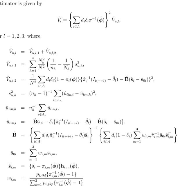
We consider two ways of estimating the variance of the proposed estimator: one is by linearization using Theorem 3.1 in Section 3.3, and the other is by the jackknife method. Firstly, the linearization variance estimator will be established using Theorem 3.1. By Theorem 3.1, the variance of the PS estimator, ˆθP S,p, can be estimated by

ˆ Vlin(ˆθP S,p) = 1 nτˆ −1_ˆ VU l( ˆτ−1)T (3.18)

where ˆτ =n−1Pn i=1δiπ −1_(x 1i, yi; ˆφ) ˙u(ˆθP S,p;xi, yi), u˙(θ;x, y) =∂u(θ;x, y)/∂θ)T, ˆ VU l = (n−1)−1 n X i=1 (ˆuli−u¯n)2, ˆ uli =uli(ˆθP S,p,φˆp,γˆ), u¯n=n−1Pn_i=1uˆli, uli(θ,φ,γ) = −Bˆs¯∗0(φ;xi,φ,γ) +δi u(θ;xi, yi) π(x1i, yi;φ) −Bˆ{s(φ;δi,x1i, yi)−¯s∗0(φ;xi,γ,φ)−κˆs1(γ;xi, yi)} , ˆ B = ( _n X i=1 δiπ−1(x1i, yi; ˆφp)u(ˆθP S,p;xi, yi)sT( ˆφp;δi,x1i, yi) ) ˆ_I−1 22( ˆφp,γˆ), ˆ κ = ˆI21( ˆφp,γˆ)ˆI−111( ˆφp,γˆ), ˆ_{I22(φ,γ) =} n X i=1 (1−δi)¯s∗0(φ;xi,φ,γ) X j;δj=1 w_ij∗(φ;γ)sT(φ;x1i, yj)/π(φ;x1i, yj), ˆ_{I21(φ,γ) =} n X i=1 (1−δi) X j;δj=1 w∗_ij(φ;γ){s(φ;δi,x1i, yj)−¯s∗0(φ;xi,φ,γ)}sT1(γ;xi, yj), ˆ_{I11(φ,γ) = −} n X i=1 δis˙1(γ;xi, yi), w∗_ij(φ,γ) is defined in (3.14), ¯s∗₀(φ;xi,φ,γ) =P_j;δj=1wij∗(φ,γ)s(φ;δi,x1i, yj),s˙(φ;δ,x, y) = ∂s(φ;δ,x, y)/∂φT_{, s˙} 1(γ;x, y) = ∂s1(γ;x, y)/∂γT,and C(y;γ) = P l;δl=1f1(y|xl;γ).

Another way to estimate the variance of the PS estimator is to use the jackknife method. Let w_i(k) be the k-th replicate weight under simple random sampling, which is defined by w(_ik) =      (n−1)−1 if i6=k 0 if i=k.

First, the k-th jackknife replicate of ˆγ, ˆγ(k) is obtained by solving S(₁k)(γ) = 0, where

S(₁k)(γ) = Pn

i=1w (k)

i δiS1(γ;xi, yi). Next, the k-th jackknife replicate of ˆφp can be

com-puted by solving S(₂k)(φ; ˆγ(k)) =0, where

S(₂k)(φ; ˆγ(k)) = n X i=1 w(_ik)    δis(φ;δi,x1i, yi) + (1−δi) X j;δj=1 w∗_ij(k)(φ,γˆ(k))s(φ;δi,x1i, yj)    , (3.19)

w(_ik) is k-th jackknife replicate weight, w_ij∗(k)(φ,γ) = w (k) i O(x1i, yj;φ)f1(yj |xi;γ)/C(k)(yj;γ) P l;δl=1w (k) i O(x1i, yl;φ)f1(yl|xi;γ)/C(k)(yl;γ) , (3.20) and C(k)_{(y;γ) =} P l:δl=1w (k) l f1(y|xl;γ).

Remark 3.1. Solving S(₂k)(φ) = 0 using the EM algorithm may involve heavy compu-tation. We can avoid this issue by approximating the solution to (3.19) by a one-step method as follows ˆ φ(_pk) = ˆφp− ( ∂S(₂k)( ˆφp) ∂φ )−1 S(₂k)( ˆφp; ˆγ(k)), where ∂S(₂k)(φ; ˆγ(k)) ∂φ = n X i=1 w_i(k)(1−δi) X j;δj=1 w∗_ij(k)(φ;γ(k))¯s∗₀(k)(φ;xi)sT(φ;x1i, yj)/π(φ;x1i, yj), ¯ s∗₀