Efficient, effective, and insightful tackling of the high-dose-rate brachytherapy treatment planning problem for prostate cancer using evolutionary multi-objective optimization algorithms

(1)

High-Dose-Rate Brachytherapy Treatment Planning Problem for

Prostate Cancer using Evolutionary Multi-Objective

Optimization Algorithms

Ngoc Hoang Luong

Centrum Wiskunde & Informatica Amsterdam, The Netherlands

[email protected]

Anton Bouter

[email protected]

Marjolein C. van der Meer

Academic Medical Center Amsterdam, The Netherlands [email protected]

Yury Niatsetski

Elekta

Veenendaal, The Netherlands [email protected]

Cees Witteveen

Delft University of Technology Delft, The Netherlands [email protected]

Arjan Bel

Academic Medical Center Amsterdam, The Netherlands

[email protected]

Tanja Alderliesten

Academic Medical Center Amsterdam, The Netherlands

[email protected]

Peter A.N. Bosman

[email protected]

ABSTRACT

We address the problem of high-dose-rate brachytherapy treatment planning for prostate cancer. The problem involves determining a treatment plan consisting of the so-called dwell times that a radi-ation source resides at different positions inside the patient such that the prostate volume and the seminal vesicles are covered by the prescribed radiation dose level as much as possible while the or-gans at risk, e.g., bladder, rectum, and urethra, are irradiated as lit-tle as possible. The problem is highly constrained, following clini-cal requirements for radiation dose distribution while the planning process for treatment planners to design a clinically-acceptable treatment plan is strictly time-limited. In this paper, we propose that the problem can be formulated as a bi-objective optimization problem that intuitively describes trade-offs between target vol-umes to be radiated and organs to be spared. We solve this problem with the recently-introduced Multi-Objective Real-Valued Gene-pool Optimal Mixing Evolutionary Algorithm (MO-RV-GOMEA), which is a promising MOEA that is able to effectively exploit de-pendencies between problem variables to tackle complicated prob-lems in the continuous domain. MO-RV-GOMEA also has the capa-bility to perform partial evaluations if problem structures allow lo-cal variations in existing solutions to be efficiently computed, sub-stantially accelerating the overall optimization performance. Ex-periments on real medical data and comparison with state-of-the-art MOEAs confirm our claims.

Permission to make digital or hard copies of all or part of this work for personal or classroom use is granted without fee provided that copies are not made or distributed for profit or commercial advantage and that copies bear this notice and the full cita-tion on the first page. Copyrights for components of this work owned by others than ACM must be honored. Abstracting with credit is permitted. To copy otherwise, or re-publish, to post on servers or to redistribute to lists, requires prior specific permission and/or a fee. Request permissions from [email protected].

GECCO ’17 Companion, Berlin, Germany

CCS CONCEPTS

•Mathematics of computing→Evolutionary algorithms;

KEYWORDS

linkage learning, multi-objective optimization, partial evaluation, brachytherapy, radiotherapy, cancer treatment planning

ACM Reference format:

Ngoc Hoang Luong, Anton Bouter, Marjolein C. van der Meer, Yury Niat-setski, Cees Witteveen, Arjan Bel, Tanja Alderliesten, and Peter A.N. Bos-man. 2017. Eﬃcient, Eﬀective, and Insightful Tackling of the High-Dose-Rate Brachytherapy Treatment Planning Problem for Prostate Cancer us-ing Evolutionary Multi-Objective Optimization Algorithms. InProceedings Companion of GECCO ’17 Companion, Berlin, Germany, July 15-19, 2017,

8 pages.

DOI: http://dx.doi.org/10.1145/3067695.3082491

1 INTRODUCTION

Radiotherapy is a frequently used form of treatment for cancer. Brachytherapy (BT) [14] is a form of internal radiotherapy where radiation sources are placed inside, or passed through, the patient’s body, close to the tumors, as opposed to the External Beam Radi-ation Therapy (EBRT) where radiRadi-ation is directed at the tumors from outside the patient’s body. A potential advantage of BT is that due to its local nature, the radioactive dose distribution can be shaped to conform to the shape of the treatment volume better, and healthy surrounding organs/tissues can thus be spared from undesired radiation risks. Furthermore, the most common way to apply BT, the so-called High-Dose-Rate (HDR) BT, is by using a ra-dioactive source with a high strength, resulting in fewer radiation treatment fractions. In this paper, we focus on HDR-BT treatment for prostate cancer but the methodology can be straightforwardly adapted to other types of BT involving radioactive sources with

(2)

a lower strength. To deliver radiation sources to the target vol-umes (i.e., the prostate, and in some cases, the seminal vesicles), normally, 14-20 catheters (depending on the prostate size) are in-serted into patient’s body through the transperineal skin. These catheters are connected to a device, called the afterloader, which controls the movement of radiation sources through the catheters. Each catheter has a certain number ofdwell positionswhere the source can pause to release radiation for a certain amount of time, termeddwell time, before moving to the next position. The longer the dwell time at a dwell position, the more radioactive dose is dis-tributed to the surrounding volume. The list of all dwell times at all dwell positions comprises an HDR-BT treatment plan. Mak-ing a clinically-acceptable BT plan is not a trivial task, and in-volves many clinical requirements that need to be satisfied. On the one hand, dwell times should be long enough to cover the target volumes as much as possible with a certain prescribed radiation dose, effectively sterilizing cancer cells. On the other hand, dwell times should be as short as possible to keep the radiation deliv-ered to normal tissues and other nearby Organs At Risk (OARs), i.e., urethra, rectum, bladder, under certain clinically-acceptable upper bounds. Aiming to cover the target volumes while sparing OARs, BT treatment planning is intrinsically a multi-objective opti-mization problem, where a singleutopiansolution (i.e., a treatment plan) that optimizes all objectives at the same time does not exist. Instead, there exists thePareto-optimalset ofnon-dominated solu-tions, that are optimal in the sense that improving any objective of these solutions deteriorates their other objectives. The image set of the Pareto-optimal set in the objective space forms the so-called Pareto-optimalfrontthat exhibits the possible trade-offs between the involved objectives. The goal then in multi-objective optimiza-tion is to find a so-called approximaoptimiza-tion set of soluoptimiza-tions that is as close as possible to the optimal Pareto set of solutions, often mea-sured in the objective space.

Available BT treatment planning software packages, see e.g., [5, 7, 10], however, do not tackle the problem in atruemulti-objective manner. Instead, all the objectives following from the clinical re-quirements are combined into a single optimization function by the weighted-sum approach, obtaining thus a single solution that corresponds with each setting of the weighting coefficient vector. The proper setting of these weights can hardly be determineda pri-oribecause it involves taking into account the geometry of the pa-tient’s organs, the configuration of the inserted catheters, and the preferences of the treating physician. Weighted-sum approaches with somerule-of-thumbcoefficient settings often return treatment plans that do not match the trade-off that individual radiation on-cologists prefer for specific patients. Therefore, BT treatment plan-ners (i.e., radiation oncologists, radiation therapy technologists, and clinical physicists) often need to spend time to manually ad-just the treatment plan until satisfied, sometimes up to an hour. In this paper, we tackle BT treatment planning in thetrue multi-objective optimization manner, approximating the set of optimal trade-offs between target volumes coverage versus OARs sparing. Such an approximation set explicitly quantifies and exhibits the compromises that need to be made. Treatment planners can make use of the obtained approximation set as a decision support tool to quickly locate the desired trade-off solution, which can be further adjusted, to arrive at a final plan.

The HDR-BT treatment procedure is time-constrained, where the planning task should normally be finalized within one hour. Optimization algorithms need to spend a certain number of itera-tions including treatment plan evaluaitera-tions before acceptable plans can be obtained. BT treatment plan evaluation is a time-consuming operation, which involves calculations of the radiation dose dis-tribution at target volumes and OARs. In this paper, we present how the dependency structure of dwell positions can be used to en-hance the efficiency in generating promising candidate treatment plans. Such dependency knowledge can be acquired online by per-forming linkage learning during the optimization process or can be computed offline based on the geometry information of the im-planted catheters. Always performing a full evaluation of treat-ment plans is unnecessary, especially if the offspring solutions dif-fer from parent solutions at only a few dwell times. Therefore, the solving time can be substantially improved if local changes of treat-ment plans can be computed. To this end, we use the recently-introduced Multi-Objective Real-Valued Gene-pool Optimal Mix-ing Evolutionary Algorithm (MO-RV-GOMEA) [2], which has been shown to have superior performance on benchmark problems due to its capabilities of exploiting linkage information and perform-ing partial evaluations in the context of continuous optimization. Here, we aim to see the impact of the advantages that MO-RV-GOMEA has to offer in solving the BT treatment planning problem compared to the well-known Multi-Objective Evolutionary Algo-rithm (MOEA) NSGA-II [4] and the Multi-Objective Estimation-of-Distribution Algorithm (MOEDA) MAMaLGaM [1].

2 PROBLEM MODELING

2.1 Clinical Practice

An HDR-BT treatment for prostate cancer starts with the insertion of a number of catheters through the area between the patient’s scrotum and anus (i.e., the perineum) aimed at target volumes (i.e., the prostate and seminal vesicles). The implanted catheters (i.e., implant) are firmly fixed to avoid displacements. Medical images (e.g., Computed Tomography (CT) or Magnetic Resonance Imag-ing (MRI) scans) of the patient’s pelvic area are then acquired to be employed in the following treatment planning session. Treat-ment planners first draw the contours of the treatTreat-ment targets and OARs on the obtained CT/MRI scans in BT treatment planning soft-ware. The inserted catheters are also delineated. Each catheter is discretized into a number of dwell positions where radiation sources can dwell, normally by a step size of 2.5mmbeginning from the first dwell position which is offset 5.0mmfrom the tip of the catheter. To ensure the treatment targets are sufficiently treated while sparing OARs from radiation risks, only dwell posi-tions within the target volumes expanded with a margin of 5.0mm

are activated. Dwell positions outside these volumes are kept inac-tive, which means they will not be considered when the treatment plan is made. The longer the time a source dwells at an active posi-tion (i.e., dwell time), the more radiaposi-tion is delivered to surround-ing tissues. A certain dose level is prescribed by radiation oncol-ogists which is deemed sufficient to sterilize tumor cells for the specific tumor type. Dwell times should then be configured such that the entire prostate should receive at least theprescribed dose,

(3)

Evolutionary Multi-Objective Optimization Algorithms GECCO ’17 Companion, July 15-19, 2017, Berlin, Germany

but not too much in order to allow healthy cells, which are less sus-ceptible to radiation than tumor cells, to recover from being radi-ated. On the one hand, treatment plans with very long dwell times can kill all tumor tissues but can also cause undesirable damage to healthy tissues (i.e., necrosis, which is considered life-threatening). On the other hand, treatment plans with too short dwell times can spare healthy tissues, but insufficiently-treated tumor cells can still grow, making the whole treatment ineffective. BT treatment plan-ners need to make a proper treatment plan that satisfies general clinical requirements as well as special criteria for each specific case. Theapprovedplan is then used to treat the patient. The after-loader, which is connected to the inserted catheters, controls the movements of the radiation source through the catheters such that the source stays at each dwell position for the amount of time as indicated in the approved plan.

2.2 Dose Distribution Evaluation

Each treatment plan (i.e., a specific configuration of dwell times) brings about a dose distribution in the surrounding tissues. A plan is deemed clinically acceptable if its dose distribution satisfies the clinical requirements. Autopianplan that radiates all tumor cells with the prescribed dose while delivering no radiation to OARs never exists. Clinical requirements therefore often indicate the sufficient lower bounds of radiating target volumes and allowable upper bounds of radiating OARs. A widely-used set of clinical requirements, termed Dose-Volume (DV)V_xo criteria (or require-ments), specify how large thecumulative volumeof an organo re-ceiving at least the radiation dose levelxshould be. For example, it is often recommended thatV₁₀₀prostate ≥ 95%, i.e., at least 95% of the prostate volume should be covered by 100% of the prescribed dose [6]. To treat tumor cells possibly existing in the vesicles, the requirementVvesicles

80 ≥ 95% can be employed to indicate that at

least 95% of the volume of the vesicles should receive 80% of the prescribed dose. To prevent hot spots forming inside the prostate (i.e., the part of prostate that is radiated too much), it is required thatV₂₀₀prostate≤20%, i.e., not more than 20% of the prostate volume should be covered by 200% of the prescribed dose. Similarly, to pro-tect OARs from radiation risks, there are DV criteria for each organ that set the upper bounds of the radiation levels that can be allowed to be delivered to that organ. For example,Vrectum

78 ≤1cm3, i.e., the

rectum volume covered by 78% of the prescribed dose should not exceed 1 cubic centimeter (cm3), orVbladder

74 ≤2cm3, i.e., the

blad-der volume receiving at least 74% of the prescribed dose should not be more than 2cm3. Table 1 presents the DV indices and their corresponding requirements currently employed at the Aca-demic Medical Center (AMC), the hospital involved in this study. tf It is impossible to calculate the radiation received by every

sin-Prostate Bladder Rectum Urethra Vesicles

V100≥95%V86≤1cm3V78≤1cm3V110≤0.1cm3V80≥95%

V150≤50%V74≤2cm3V74≤2cm3

V200≤20%

Table 1: BT treatment planning DV criteria at AMC.

gle cell because the number of cells in an organ is prohibitively large. Therefore, DV index values are often approximated by eval-uating the radiation at a certain number of so-calleddose calcula-tion points. The strength of the employed radiation source and the

relative position between a dwell position and a dose calculation point determine thedose ratethat indicates the amount of dose ir-radiated from the source when it resides at that dwell position to the dose calculation point per second (i.e., Gy/s). Dose rates can be computed based on the TG-43 protocol (the American Association of Physicists in Medicine AAPM Task Group No. 43 Report) [12]. The total radiation at each dose calculation point is the combined dose delivered from all the active dwell positions corresponding to the dwell times of the treatment plan. LetDbe the set of all dose calculation points,|D|₌nD. LetTbe the set of all dwell positions,

|T|₌nT. With a certain source strength,Ris annD×nT matrix

whereR_{i j}_{indicates the dose rate associated with dwell position}_j and dose calculation pointi. Lett_{be the vector of dwell times at} all active dwell positions (i.e.,t_{is a treatment plan). The vector}d of the amounts of radiation received at all dose calculation points can be computed as:

d₌Rt ₍₁₎

The vectord_{can be seen as representing the dose distribution} as-sociated with the treatment plant, from which the DV indices (in Table 1) can be approximated. The dose calculation points can be uniformly randomly generated inside each organ. LetDo be the

set of all dose calculation points inside organo,Do ⊂D. The DV

indexVxoin relative terms (%) can then be computed as:

Vxo = 1 |Do| X i∈Do χ(di,x) (2)

wherediis the total amount of radiation received at the dose

cal-culation pointi, andχ(di,x)is an indicator function:

χ(di,x)=

(

1 di ≥x

0 di <x (3)

The DV indexVxoin absolute terms (cm3) can be straightforwardly

computed by multiplying the result from Equation 2 with the to-tal volume of the organo. The more dose calculation points are used, the more accurate the approximation of the true DV indices is (disregarding uncertainties of delineation). However, using a large number of dose calculation points incurs a substantial amount of computing time, which slows down the planning process.

2.3 Optimization Constraints

BT treatment planners normally start the planning process from an initial plan, which is generated by BT treatment planning software [7, 10]. Because of the diﬃculty in directly optimizing DV indices due to their discrete nature (Equation 2), planning software often solves simpler optimization models of the problem. Therefore, DV requirements (in Table 1) are not always satisﬁed by the proposed plans. Planners need to identify the causes of the violated require-ments and then manually adjust the plan in a local manner (i.e., changing the values of some dwell times). For example, dwell times at dwell positions inside the under-radiated part of the prostate volume can be increased ifV₁₀₀prostate<95%. If the plan causes many hot spots, then very long dwell times can be decreased to reduce

V₂₀₀prostate. Planners often improve DV indices one by one, giving pri-ority to the most violated criteria. Making a DV index satisfy its re-quirement, however, can deteriorate other indices and might make them violate their requirements. For example, increasingV₁₀₀prostate

(4)

can create new hot spots (i.e., large values ofV₂₀₀prostate) and cause other DV indices for OARs to exceed their recommended thresh-olds. How good the best possible treatment plan is depends on the quality of the implant (i.e., how well the catheters are inserted) and also on the geometry of the surrounding organs. When OARs are too close to target volumes, it is diﬃcult to achieve good DV in-dex values for both target coverage and OARs sparing at the same time. If the catheters are not inserted deep enough, it might be im-possible to obtainV₁₀₀prostate ≥95% without violatingV₂₀₀prostate ≤20%. In these situations, BT treatment planners need to compromise. To allow treatment plans that violate some part of the clinical require-ments to some degree to be obtained in the optimization process, we relax the thresholds of the DV requirements to enlarge the fea-sible search space. Speciﬁcally, the upper bounds of organ sparing indices are increased four times. For example,Vbladder

74 ≤2cm3in

the original clinical requirement becomesVbladder

74 ≤ 8cm3. The

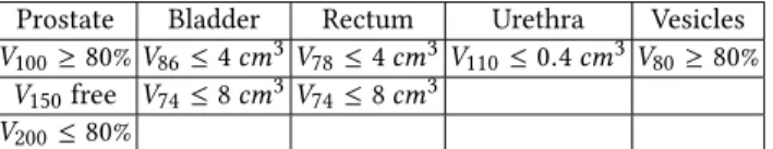
lower bounds of target coverage indices are also decreased in a similar manner, e.g.,V₁₀₀prostate ≥95% becomesV₁₀₀prostate≥80%. These relaxed requirements, presented in Table 2, are the constraints in our optimization model.

Prostate Bladder Rectum Urethra Vesicles

V100≥80%V86≤4cm3V78≤4cm3V110≤0.4cm3V80≥80%

V150free V74≤8cm3V74≤8cm3

V200≤80%

Table 2: DV criteria from Table 1 with relaxed feasibility thresholds. Because of the relaxation factor,V₁₅₀prostatehas be-come unconstrained.

2.4 Multi-Objective Optimization

BT treatment planning is a multi-objective optimization problem, where each DV index criterion can be considered to be an optimiza-tion objective. Optimizing target coverage indices (i.e.,V₁₀₀prostate,

Vvesicles

80 ) equals making them as large as possible (above the lower

bound thresholds) while optimizing organ sparing indices (the re-maining indices in Table 1) equals making them as small as possible (under the upper bound thresholds). These two groups of DV in-dices are conflicting with each other. Each treatment plan can be seen as a trade-off between all the involved indices. Of key inter-est is to find the set of optimal trade-offs, termednon-dominated solutions, where improving any DV index in one group worsens DV indices in the other group. It is beneficial for the planners to be informed about these best possible alternatives before approving a plan to be used for treating the patient.

However, optimizing all DV indices of Table 2 as separate objec-tives would result in an 8-objective optimization problem, which is difficult to be efficiently solved. Moreover, its resulting set of 8-dimensional trade-offs is also complicated to be visualized and interpreted. On the other hand, simply summing all indices of a group into an objective is also not favorable since this also re-duces the insight into key information about DV indices, namely the minimally achieved levels. We therefore propose a bi-objective optimization model that retains important insights in trade-offs be-tween DV indices. The two objectives are: theLeast Coverage In-dex(LCI), which corresponds to the worst-scored DV index in the target coverage group, and theLeast Safe Index(LSI), which corre-sponds to the worst-scored DV index in the organ sparing group.

For a candidate treatment plant, its LCI value can be considered as:

LCI(t)=min{V₁₀₀prostate,V₈₀vesicles} (4) The value of LCI, that we would like to maximize, is∈ [0,1]. The value 0 indicates that one target volume (i.e., prostate or semi-nal vesicles) has no dose calculation point covered by the recom-mended dose level for that target volume. The ideal value 1 indi-cates that the whole volume of each treatment target is covered by the recommended dose level. The value 0.95 indicates thatboth clinical requirementsV₁₀₀prostate ≥95% andVvesicles

80 ≥95% in Table 1

are satisﬁed. LetVo,max

x be the upper bound threshold for the dose levelx

to the organoin Table 2. The further the value of DV indexVxois

below this threshold, the better the organois spared from radiation risk. The distance of an organ sparing indexVxo value below the

thresholdVo,max

x can be measured and normalized as:

δ(Vxo)=1− V o x Vo,max x (5) The LSI of a candidate treatment plant_{can then be deﬁned as:}

LSI(t)₌min{δ(V₁₅₀prostate),δ(V₂₀₀prostate),δ(Vbladder

86 ),δ(V74bladder),

δ(V78rectum),δ(V74rectum),δ(V110urethra)}

(6) The value of LSI, that we would like to maximize, is∈[0,1]. The value 0 indicates that one organ sparing indexVxois currently at its

(relaxed) thresholdVo,max

x . The ideal value 1 indicates that there

is no dose calculation point in any organ receiving more radiation than its relaxed threshold dose level. Since the upper bounds of all organ sparing indices are increased (i.e., relaxed) by a factor of 4, the value LSI= 0.75 ensures that all clinical requirements for organ sparing indices in Table 1 are met.

The objective values of any candidate treatment plan can thus be evaluated on these two objectives (LCI, LSI), where it can be inferred that the values of all the other DV indices in a group are at least as good as the representative index of that group. A treat-ment plan satisﬁes all original clinical requiretreat-ments in Table 1 if its LCI≥0.95 and LSI≥ 0.75. We further argue that this model bears resemblance with the treatment planning process in practice in the sense that planners often try to iteratively improve the most violated DV index.

3 MO-RV-GOMEA

MO-RV-GOMEA [2] maintains a population of potential solutions on which selection and variation are performed. Encountered non-dominated solutions are stored in an adaptive elitist archive [11]. A key strength of MO-RV-GOMEA is the main variation operator that was ﬁrst introduced for the discrete GOMEA [13], and was later adapted to the domain of real-valued variables [2]. This varia-tion operator was shown to be able to successfully exploit linkage structure in a wide range of optimization problems [2, 13].

Each generation of MO-RV-GOMEA starts with the selection phase, where the selection is based on the ranking of solutions after non-domination sorting [4]. The selection is then partitioned into a set of clusters, which will allow diﬀerent directions of optimization in diﬀerent parts of the Pareto front. For each objective of interest, this set of clusters contains one so-called single-objective cluster

(5)

Evolutionary Multi-Objective Optimization Algorithms GECCO ’17 Companion, July 15-19, 2017, Berlin, Germany

for which the selection procedure only considers the respective objective. Apart from the selection, each solution in the population is also assigned to a nearby cluster, because the Gaussian model of one speciﬁc cluster is used in the variation of the solution.

A linkage model is used to explicitly define dependencies be-tween subsets of variables. Each linkage model consists of a num-ber of linkage sets, where each linkage set describes a subset of variables that are considered to be dependent. The linkage tree is a specific hierarchical linkage model that models a range of de-pendencies ranging from low-level to high-level dede-pendencies. A linkage tree can be learned during optimization, in which case it is learned anew at the start of each generation. The linkage tree is initialized as a set ofℓleaves of univariate problem indices. New nodes are added to the tree by iteratively merging the two non-merged nodes that are considered the most dependent by a sim-ilarity metric, for which we use the mutual information metric, which is derived from the sample Pearson correlation coefficient [8]. Alternatively, a similarity metric can be defined based on the structure of the optimization problem, leading to a linkage tree that is fixed throughout all generations. Merging nodes continues until the root of the tree has been created, which naturally contains the indices of all problem variables. Each node of the linkage tree then defines one linkage set of the linkage model.

The parameters for variation are estimated as follows. For each linkage set of each cluster, a multivariate Gaussian probability dis-tribution is estimated with maximum likelihood based on the se-lection. The probability distribution of a certain linkage set covers only the variables that are included in this linkage set. A distri-bution multiplier is also maintained for each linkage set, which allows the dynamic adaptation of the size of each Gaussian kernel based on the observed direction of improvement. Per linkage set of each cluster, the variation operation is applied to each solution in this cluster by sampling new values from the Gaussian distribu-tion for the problem variables described by the respective linkage set, and inserting these into the solution. A fraction of the solu-tions in each cluster is shifted by the application of the Anticipated Mean Shift (AMS), which shifts parameters by a factor relative to the generational difference of means. The modification of the solu-tion is then evaluated, but only maintained if this modificasolu-tion is considered to be an improvement. Otherwise, the modification is not accepted and the solution is returned to its previous state.

We refer the interested reader to [2] for a full description of MO-RV-GOMEA.

4 PERFORMANCE ENHANCEMENT

4.1 Exploiting Geometry Information

MO-RV-GOMEA performs variations based on linkage models that indicate which problem variables (i.e., in this case, dwell times at dwell positions) exhibit some degree of dependency and should thus be treated together. In the context of black-box optimiza-tion, linkage models can be learned from the population. Although even the most comprehensive linkage model employed by MO-RV-GOMEA, i.e., the linkage tree, can be efficiently learned, perform-ing linkage learnperform-ing in every cluster for each generation can incur some computing time overhead. It could be beneficial and more efficient if sufficient problem-specific information is available to

construct the linkage models offline. For the BT treatment plan-ning problem, it can be argued that dwell positions that are close to each other have stronger interactions than dwell positions that are far apart. Dwell times at neighboring dwell positions, therefore, should be treated together when performing variation. The coor-dinates of all active dwell positions, which are determined from the CT/MRI scans of the patients, can be used to compute the Eu-clidean distances between all pairs of dwell positions. Such ge-ometry information can be directly used as a distance/similarity metric to construct the linkage tree as in Section 3. This offline-constructed Euclidean-distance-based linkage tree can be employed during the optimization process without the need of online linkage learning in each cluster, potentially improving the effectiveness in creating promising candidate treatment plans.

4.2 Partial Evaluations

(MO-RV-)GOMEA differs from other evolutionary algorithms in its genetic-local-search-like variation operator that transforms each existing (parent) solution into a new (offspring) solution in a step-wise manner. At each step, a few problem variables’ values (i.e., dwell times in this context) are altered, and the changes are only ac-cepted if they improve the quality of the current solution (i.e., the candidate treatment plan at hand). Which problem variables are varied at each step is often determined by the linkages described by the employed linkage model such that variables having some degree of dependency should be jointly treated. In black-box op-timization, each partially-altered solution needs to be fully evalu-ated to check for improvements. If the problem is sufficiently un-derstood, the impact of such local changes can be efficiently com-puted/approximated using partial evaluations. The evaluation of a treatment plan involves the computing of the radiation dose re-ceived at each dose calculation point (see Equation 1) and the com-puting of DV indices (see Equation 2). The former takes a more substantial amount of computing time. The matrix-vector multi-plication in Equation 1, however, does not need to be calculated completely anew when the vector of dwell times is changed at only a few elements (i.e., dwell positions). More specifically, the impact of such changes on the dose distribution can be efficiently computed by invoking only the columns of the dose-rate matrixR corresponding with the dwell positions where the dwell times are altered. Lettbe an evaluated treatment plan with the correspond-ing dose distributiond_{. Let}t′_{be a treatment plan that differs from} t_{at only a few dwell positions, i.e.,}t′

=t+∆t, in which∆thas

many zero elements. The dose distributiond′_{associated with}t′ can be computed as:

d′₌Rt′₌R(t₊∆t)₌Rt₊R∆t₌d₊R∆t ₍₇₎ where thei-th index ofR∆t_{can be computed as:}

(R∆t)i = nT X j=1 ∆tj,0 R_{i j}∆tj (8)

which thus only involves the multiplication of the columnR_∗_j_of R_{with the corresponding non-zero elements}∆tjof∆t. Note that

in the implementation an entire vector∆t _{is not explicitly} com-puted, but rather only the compact vector of non-zero elements in ∆tcorresponding to a linkage set in the linkage tree is computed.

(6)

The step-wise operation of the variation operator of MO-RV-GOMEA makes it straightforward for partial evaluations to be em-ployed, if possible. For other existing MOEAs, such as MAMaL-GaM or NSGA-II, each time a whole oﬀspring solution is created at once, making partial evaluations impossible.

5 EXPERIMENTS

5.1 Experiment Settings

DICOM files of three anonymized HDR-BT cases for prostate can-cer from the Academic Medical Center (AMC) were available for conducting our experiments. DICOM files are loaded into the BT treatment planning software Oncentra Brachy, from which the con-tours of the involved organs (i.e., prostate, seminal vesicles, blad-der, rectum, and urethra) and the inserted catheter information can be exported. This extracted information is then used as the input data for our multi-objective optimization algorithm. Similar to clin-ical practice, we activate all dwell positions inside the two target volumes: the prostate and seminal vesicles, each with an extended margin of 5mmwhile dwell positions within 1mmmargin of the urethra should be kept inactive. In each organ, we uniformly ran-domly generate 4,000 points, i.e., a total of 20,000 dose calculation points are employed each time. Such a number of random points is deemed sufficient for the purpose of performing optimization [9]. We perform experiments with three MO-RV-GOMEA variants employing three linkage models: the Univariate Factorization (UF) model where all dwell times are deemed independent from each other, the Linkage Tree (LT) model which is learned from the pop-ulation in each generation, and the fixed LT which is constructed a prioribased on the geometry information of active dwell po-sitions. For each MO-RV-GOMEA we run two settings: 1) full treatment plan evaluations are always carried out to assess can-didate treatment plans, and 2) partial evaluations are enabled to assess partially-altered treatment plans when performing solution variation. For the purpose of performance comparison between MO-RV-GOMEA and state-of-the-art MOEAs, we consider NSGA-II [4] and MAMaLGaM [1]. NSGA-NSGA-II employs the Simulated Binary Crossover (SBX [3, 4]) operator to create offspring solutions in real-valued optimization. MAMaLGaM estimates a Gaussian mixture distribution over the 35% best solutions in the population and sam-ples the learned distribution to generate offspring solutions in each generation. To eliminate the tuning of the population size param-eter, for all algorithms, we implement the interleaved multistart scheme as introduced in [2]. For every patient case, we run each al-gorithm 30 times independently. Each optimization run is allowed to operate 1 hour to obtain an approximation set of non-dominated plans.

We use the hypervolume [15] to compare the performance of MOEAs. The hypervolume can be intuitively deﬁned as the volume (or area in the case of bi-objective optimization) in the objective space that is covered by a set of non-dominated solutions and a referencepoint, which is a point that can be selected such that it will be dominated by any possible solutions. Here, since the range of the two objectives LCI and LSI is [0,1], we can simply choose (−0.1,−0.1)as the reference point.

5.2 Results

Figure 1 shows the graphs of hypervolume development along the running time (in seconds) averaged over 30 runs of each optimiza-tion algorithm for the three patient cases. To support some of our observations from the figure, we use the Mann-Whitney-Wilcoxon statistical hypothesis test for equality of medians withp<0.05 to see whether the final result obtained by one algorithm is statisti-cally different from that of another algorithm. When partial eval-uations are not enabled, i.e., MO-RV-GOMEA carries out a normal full evaluation every time a candidate solution needs to be assessed, all MO-RV-GOMEA variants are outperformed by both NSGA-II and MAMaLGaM. Using totally full evaluations is inefficient for MO-RV-GOMEA because treatment plan evaluation is a compu-tationally expensive operation and the algorithm most often only modifies an existing solution in a few variables at each step before fully constructing a new (offspring) solution, which differs from other MOEAs like NSGA-II and MAMaLGaM that generate a whole new solution at once. While the slopes of the hypervolume devel-opment graphs of NSGA-II and MAMaLGaM flatten out at the end of the optimization runs, suggesting that both algorithms nearly converge, the ones of MO-RV-GOMEA variants still steepen up, indicating that they are still in the middle of the search. Note that using different linkage models that capture only higher-order de-pendencies of a certain minimum degree could have a substantial impact here and make the difference much smaller. However, us-ing partial evaluations, as is possible here, could make such search for highly suitable linkage structures superfluous.

Indeed, when partial evaluations are enabled, all variants of MO-RV-GOMEA are substantially accelerated, outperforming both MA-MaLGaM and NSGA-II in the cases of patients 2 and 3. At the termination time of one hour, in all three cases, MO-RV-GOMEA with the fixed LT and partial evaluations is the best algorithm, ob-taining Pareto fronts with the highest hypervolume values, which are found to be statistically significantly different from the other MO-RV-GOMEA variants and the other MOEAs. Therefore, we consider the fixed LT with partial evaluations as the most suitable configuration for MO-RV-GOMEA to tackle the BT treatment plan-ning problem and we only consider this configuration in the fol-lowing discussion.

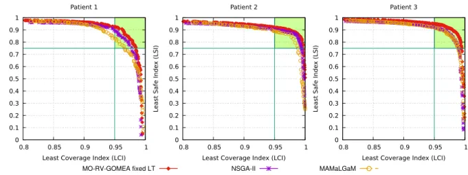
Figure 2 shows the Pareto fronts of non-dominated plans ob-tained by NSGA-II, MAMaLGaM, and MO-RV-GOMEA for the 3 cases. Each Pareto front is the combination of the 30 approxima-tion sets obtained at the end of the 30 optimizaapproxima-tion runs of each algorithm. Our formulations of the two objectives LCI and LSI (see Section 2.4) imply that treatment plans satisfying all clinical requirements (in Table 1) should equal to, or (Pareto-)dominate, the point(0.95,0.75). Graphically, clinically-acceptable treatment plans can be located in the top-right corner of the graphs between (0.95,0.75)and(1,1). Pareto fronts shown in Figure 2 indicate that treatment plans that satisfy all clinical requirements are achievable in all three cases. The Pareto fronts obtained by MO-RV-GOMEA are always better than the ones obtained by NSGA-II and MAMaL-GaM. It can be clearly seen that in the clinically-acceptable cor-ner, the solutions of MO-RV-GOMEA (Pareto-)dominate the solu-tions of both NSGA-II and MAMaLGaM, suggesting that exploiting the information of linkages between problem variables (i.e., dwell

(7)

Evolutionary Multi-Objective Optimization Algorithms GECCO ’17 Companion, July 15-19, 2017, Berlin, Germany 1 1.02 1.04 1.06 1.08 1.1 1.12 1.14 1.16 1.18 1.2 60 600 1200 1800 2400 3000 3600 Hypervolume Seconds Patient 1 1 1.02 1.04 1.06 1.08 1.1 1.12 1.14 1.16 1.18 1.2 60 600 1200 1800 2400 3000 3600 Seconds Patient 2 1 1.02 1.04 1.06 1.08 1.1 1.12 1.14 1.16 1.18 1.2 60 600 1200 1800 2400 3000 3600 Seconds Patient 3 MO-RV-GOMEA UF MO-RV-GOMEA UF (full) MO-RV-GOMEA LT MO-RV-GOMEA LT (full) MO-RV-GOMEA fixed LT MO-RV-GOMEA fixed LT (full) NSGA-II MAMaLGaM

Figure 1: The average hypervolume values of the Pareto fronts of optimization algorithms over time.

0 0.1 0.2 0.3 0.4 0.5 0.6 0.7 0.8 0.9 1 0.8 0.85 0.9 0.95 1 L

east Safe Inde

x (LSI)

Least Coverage Index (LCI) Patient 1 0 0.1 0.2 0.3 0.4 0.5 0.6 0.7 0.8 0.9 1 0.8 0.85 0.9 0.95 1 L

east Safe Inde

x (LSI)

east Safe Inde

x (LSI)

Least Coverage Index (LCI) Patient 3

MO-RV-GOMEA fixed LT NSGA-II MAMaLGaM

Figure 2: Pareto fronts combined from 30 optimization runs of each algorithm after running for 1 hour.

times) beneﬁts the optimization algorithm in reaching treatment plans of higher quality.

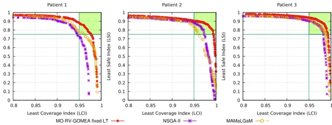
Since the treatment planning process in practice is highly time-constrained, which should not take more than 1 hour, it is inter-esting to investigate the results of optimization algorithms with a shorter time span. Figure 3 shows the Pareto fronts combined from 30 optimization runs of each algorithm after running for 10 min-utes. It can be seen that, in all three cases, MO-RV-GOMEA can ob-tain Pareto fronts of high-quality treatment plans much faster than NSGA-II and MAMaLGaM. Especially in the clinically-acceptable corner, the treatment plans found by MO-RV-GOMEA clearly dom-inate the results of NSGA-II and MAMaLGaM. Comparing Figure 2 and Figure 3, the improvements of the Pareto fronts of MO-RV-GOMEA are not as substantial as the improvements of the Pareto fronts of NSGA-II and MAMaLGaM obtained by an extra 50 minute runtime. This suggests that MO-RV-GOMEA can simply be run in only 10 minutes to achieve the results of the other MOEAs running for 1 hour. Overall, the results appear very promising. As a ﬁrst

next step, these sets of treatment plans exhibiting natural trade-oﬀs in BT treatment planning will be analyzed with clinical ex-perts and rigorously compared with clinically-approved treatment plans.

6 CONCLUSION

In this paper, we presented how the BT treament planning problem can be formulated and tackled by a novel multi-objective optimiza-tion approach in which only two objectives are considered, rather than having a single objective for each clinical objective that is typi-cally found in clinical requirements. In particular, those clinical jectives that express to maximize irradiation are grouped in one ob-jective, as are those that express to minimize irradiation. By care-fully remapping these clinical objectives and using the worst one in each group as the value in the bi-objective optimization function, a risk-averse, guaranteed minimal performance model is obtained such that the results of which are straightforward to interpret. We

(8)

0 0.1 0.2 0.3 0.4 0.5 0.6 0.7 0.8 0.9 1 0.8 0.85 0.9 0.95 1 L

east Safe Inde

x (LSI)

east Safe Inde

x (LSI)

east Safe Inde

x (LSI)

Least Coverage Index (LCI) Patient 3

MO-RV-GOMEA fixed LT NSGA-II MAMaLGaM

Figure 3: Pareto fronts combined from 30 optimization runs of each algorithm after running for 10 minutes.

proposed that the recently-introduced MO-RV-GOMEA, a promis-ing optimizer that can exploit hierarchical linkages between prob-lem variables, is an especially promising optimizer to tackle the problem because MO-RV-GOMEA allows partial evaluations to be carried out when existing solutions are only locally altered at a few variables, we suggested that this feature can be exploited us-ing the dependencies between dwell positions and their geometry information. Using linkage exploitation and partial evaluations, MO-RV-GOMEA is capable of outperforming both the widely-used MOEA NSGA-II and the state-of-the-art MOEDA MAMaLGaM in obtaining a set of high-quality treatment plans in a 1/6 fraction of the planning time budget. This, together with the fact that Pareto fronts are obtained that insightfully visualize the main trade-oﬀ in BT treatment planning, leads us to conclude that MO-RV-GOMEA is a very promising algorithm to develop and use further for the automated design of BT treatment plans.

ACKNOWLEDGMENTS

This work is part of the research programme IPPSI-TA with project number 628.006.003, which is financed by the Netherlands Organ-isation for Scientific Research (NWO) and Elekta. The authors fur-ther acknowledge the financial support provided by the Maurits en Anna de Kock Stichting for a high-performance computing system. The authors would like to thank Dr. Niek van Wieringen (Depart-ment of Radiation Oncology, Academic Medical Center, Amster-dam, The Netherlands) for his support in providing the patient data and Dr. Rob van der Laarse (Quality Radiation Therapy B.V., Zeist, The Netherlands) for his advice on radiation dose calculation.

REFERENCES

[1] P. A. N. Bosman. 2010. The anticipated mean shift and cluster registration in mixture-based EDAs for multi-objective optimization. InGenetic and Evolution-ary Computation Conference, GECCO 2010, Proceedings, Portland, Oregon, USA, July 7-11, 2010. 351–358.DOI:http://dx.doi.org/10.1145/1830483.1830549 [2] A. Bouter, N. H. Luong, C. Witteveen, T. Alderliesten, and P. A. N. Bosman. 2017.

The Multi-Objective Real-Valued Gene-Pool Optimal Mixing Evolutionary Algo-rithm. InGenetic and Evolutionary Computation Conference, GECCO ’17, Berlin, Germany, July 15-19, 2017.

[3] K. Deb. 2001.Multi-Objective Optimization Using Evolutionary Algorithms. John Wiley & Sons, Inc. http://dl.acm.org/citation.cfm?id=559152

[4] K. Deb, A. Pratap, S. Agarwal, and T. Meyarivan. 2002. A fast and elitist multi-objective genetic algorithm: NSGA-II.IEEE Transactions on Evolutionary Com-putation6, 2 (Apr 2002), 182–197. DOI:http://dx.doi.org/10.1109/4235.996017 [5] A. M. Dinkla, R. van der Laarse, E. Kaljouw, Bradley R. P., K. Koedooder, N. van

Wieringen, and A. Bel. 2015. A comparison of inverse optimization algorithms for HDR/PDR prostate brachytherapy treatment planning.Brachytherapy14, 2 (2015), 279–288.DOI:http://dx.doi.org/10.1016/j.brachy.2014.09.006 [6] P. J. Hoskin, A. Colombo, A. Henry, P. Niehoﬀ, T. P. Hellebust, F. A. Siebert, and

G. Kovacs. 2013. GEC/ESTRO recommendations on high dose rate afterloading brachytherapy for localised prostate cancer: An update.Radiotherapy and Oncol-ogy107, 3 (2013), 325–332.DOI:http://dx.doi.org/10.1016/j.radonc.2013.05.002 [7] A. Karabis, S. Giannouli, and D. Baltas. 2005. 40 HIPO: A hybrid inverse

treat-ment planning optimization algorithm in HDR brachytherapy.Radiotherapy and Oncology76 (2005), S29.DOI:http://dx.doi.org/10.1016/S0167-8140(05)81018-7 [8] A. Kraskov, H. St¨ogbauer, and P. Grassberger. 2004. Estimating mutual

information. Physical Review E 69 (Jun 2004), 066138. Issue 6. DOI: http://dx.doi.org/10.1103/PhysRevE.69.066138

[9] M. Lahanas, D. Baltas, S. Giannouli, N. Milickovic, and N. Zamboglou. 2000. Generation of uniformly distributed dose points for anatomy-based three-dimensional dose optimization methods in brachytherapy.Medical Physics27, 5 (2000), 1034–1046.DOI:http://dx.doi.org/10.1118/1.598970

[10] E. Lessard and J. Pouliot. 2001. Inverse planning anatomy-based dose optimiza-tion for HDR-brachytherapy of the prostate using fast simulated annealing al-gorithm and dedicated objective function.Medical Physics28, 5 (2001), 773–779. DOI:http://dx.doi.org/10.1118/1.1368127

[11] N. H. Luong and P. A. N. Bosman. 2012. Elitist Archiving for Multi-Objective Evolutionary Algorithms: To Adapt or Not to Adapt. In Par-allel Problem Solving from Nature - PPSN XII - 12th International Confer-ence, Taormina, Italy, September 1-5, 2012, Proceedings, Part II. 72–81. DOI: http://dx.doi.org/10.1007/978-3-642-32964-7 8

[12] R. Nath, L. L. Anderson, G. Luxton, K. A. Weaver, J. F. Williamson, and A. S. Meigooni. 1995. Dosimetry of interstitial brachytherapy sources: Recommenda-tions of the AAPM Radiation Therapy Committee Task Group No. 43.Medical Physics22, 2 (1995), 209–234.DOI:http://dx.doi.org/10.1118/1.597458 [13] D. Thierens and P. A. N. Bosman. 2011. Optimal Mixing

Evolution-ary Algorithms. In Proceedings of the 13th Annual Conference on Ge-netic and Evolutionary Computation (GECCO ’11). ACM, 617–624. DOI: http://dx.doi.org/10.1145/2001576.2001661

[14] J. L. M. Venselaar, D. Baltas, P. Hoskin, and A. S. Meigooni. 2012. Introduction and Innovations in Brachytherapy. InComprehensive Brachytherapy. Taylor & Francis, 3–8.DOI:http://dx.doi.org/doi:10.1201/b13075-3

[15] E. Zitzler and L. Thiele. 1998. Multiobjective optimization using evolu-tionary algorithms — A comparative case study. InParallel Problem Solv-ing from Nature PPSN V: 5th International Conference Amsterdam, The Nether-lands September 27–30, 1998 Proceedings, A. E. Eiben, T. B¨ack, M. Schoe-nauer, and H. P. Schwefel (Eds.). Springer Berlin Heidelberg, 292–301. DOI: http://dx.doi.org/10.1007/BFb0056872