Specific Task Training Program Course S-33 Soils Field Testing and Inspection: Course Reference Manual

(1)

Specific Task Training Program

Course S-33

Soils Field Testing and Inspection:

Course Reference Manual

(2)

(3)

Specific Task Training Program

Course S 33

Soils Field Testing and Inspection

Course Reference Manual

Prepared and Published by

Illinois Department of Transportation

Bureau of Materials and Physical Research

Springfield, Illinois

(4)

(5)

DOCUMENT CONTROL

The Specific Tasks Training Program Course S 33: Soils Field Testing and Inspection Course Reference Manualis reviewed during use for adequacy and updated as necessary by the Bureau of Materials and Physical Research. The approval process for changes to this manual is conducted in accordance with the procedures outlined in the Illinois Department of Transportation’s, Document Management Manual.

Electronic

Portable Document Format (PDF) has been selected as the primary distribution format. The official version of the manual is available on the Illinois Department of Transportation website and the Policy and Research Center Library site on InsideIDOT.

Hard Copy

The current version of this manual is distributed in hard copy format as a training aid for each class. Users who choose to print a copy of the manual are responsible for ensuring use of the most current version.

Archived Copies

Archived versions of this manual are available to examine by contacting the Bureau of Materials and Physical Research or the Policy and Research Center at [email protected].

Revision History

Revision Date Description Approval

November 20, 2013 Reissued with minor content and editorial revisions for the 2013-2014 class season.

Daniel Tobias October 24, 2014 Minor content and editorial revisions for the

2014-2015 class season including updates to discussion in Sections 4 and 8.1, class problems, figures, tables, forms, IDOT website addresses, and references.

Daniel Tobias

(6)

(7)

COURSE REQUIREMENTS FOR

SUCCESSFUL COMPLETION

Student must attend all class sessions.

• PREREQUISITE COURSES — None.

• WRITTEN TEST — The test consists of two written parts. Each part will be given at the conclusion of each section of the course: Part A “Soils Field Testing” and Part B “Field Inspection”. Both parts are open book. The time limit is 1 hour for each section. A minimum composite grade of 70 is required.

Note: The Department has no out-of-state reciprocity for this course.

• WRITTEN RETEST — If the student fails the written test, one retest can be performed. The retest is open book. The time limit is 2 hours. A minimum grade of 70 is required. A retest will not be given on the same day as the initial test. A retest must be taken by the end of the academic year that the initial test was taken. The academic year runs from September 1st of one year to August 31st of the next year. (For example, if the test was taken January 24, 2013, the last date to retest is August 31, 2013.) Failure of a written retest, or failure to comply with the academic year retest time limit, shall require the student to retake the class and the test.

• NOTIFICATION — The student will be notified by e-mail with instructions on how to

access the IDOT Learning Management System (http://www.ildottraining.org/ihtml/application/student/interface.idot/index.htm) to obtain the test results. A certificate of completion will be issued if the student passes the course, and 12 professional development hours earned with this course. Once trained, the Department does not require the individual to take the class again.

• Successful completion is required as part of the IDOT process for compliance with the Code of Federal Regulations, 23 CFR 637 and for consultant prequalification in Quality Assurance Testing according to IDOT Policy MAT-15, Quality Assurance Procedures for Construction.

(8)

(9)

APPENDICES... 61 APPENDIX A: TEST PROCEDURES COVERED IN THIS COURSE ... A-1 APPENDIX B: PPG MISTIC TESTS AND TESTING FREQUENCY ... B-1 APPENDIX C: FORMS & IDH CHART ... C-1 Moisture-Density Worksheet ... C-1 Dynamic Cone Penetration Test Form ... C-2 Static Cone Penetration Test Form ... C-3 Field Soil Compaction (Nuclear) Form ... C-4 IDH Textural Classification Chart ... C-5

(11)

List of Figures

Figure 1. Proctor Curve showing the relationship between moisture content and dry density. ... 7

Figure 2. Example of determining Standard Dry Density based on One-Point Proctor data...14

Figure 3. Nuclear Gauge Test Illustrating Direct Transmission and Backscatter Procedures. ...16

Figure 4. Sand Cone Test Apparatus. ...17

Figure 5. Dynamic Cone Penetrometer (DCP). ...20

Figure 6. Detail of cone tip of the Dynamic Cone Penetrometer (DCP). ...21

Figure 7. Static Cone Penetrometer (SCP). ...22

Figure 8. Pocket Penetrometer. ...23

Figure 9. Rutting and pumping under proof rolling or construction traffic. ...30

Figure 10. Effect of Moisture Content on IBV. ...30

Figure 11. Thickness design as a function of IBV, Cone Index (CI), Shear Strength, and Qu for subgrade treatment (granular backfill or modified soil). ...32

Figure 12. Embankments constructed over existing pavement. ...39

Figure 13. Use of restricted material in embankment. ...43

Figure 14. Stepping & Benching Placement. ...44

Figure 15. Minimum Percent (%) Compaction Requirements Based on Location in the Embankment. ...46

Figure 16. Sample settlement plate data and convergence diagram. ...51

Figure 17. Example determination of actual construction waiting period. ...51

(12)

List of Tables

Table 1. IDH Particle Size Limits of Soil Constituents defined in AASHTO M 146 ... 3

Table 2. Correlation between DCP Penetration Rate, IBV, and Qu...21

Table 3. Correlation between Cone Index, IBV, and Qu. ...23

Table 4. Aggregate Subgrade Gradations. ...28

Table 5. Improved Subgrade Thickness Requirements. ...31

Table 6. Guideline for Aggregate Thickness Reduction Using Geosynthetics. ...31

Table 7. Problematic embankment construction materials...42

Table 8. Reduction Factors (RF) for various footing widths (B) at 60 degree load distribution for over excavation depths (D). ...55

(13)

PART A: SOILS FIELD TESTING

1. INTRODUCTION, OBJECTIVES, AND KEY DOCUMENTS

1.1 Introduction

The Specific Task Training Program Course, S 33, “Soils Field Testing and Inspection”, has been prepared to provide basic guidance to construction and materials personnel involved in field testing and inspection of soils and rock. For the purpose of this document, field personnel will be referred to as “Inspector” and the District Geotechnical Engineer will be referred to as “Geotechnical Engineer”. Inspections include excavation, embankment, subgrade, and shallow foundations for various structures. This course also describes common problems and the remedial actions generally used to correct them.

1.2 Course Objectives

In this course, the Inspector will learn how to:

• Determine field moisture content along with in-situ wet and (corresponding) dry densities

• Determine Standard Dry Density (SDD) and Optimum Moisture Content (OMC) using the Family of Curves and One-Point Proctor

• Determine percent compaction and percent of OMC

• Determine soil stability and strength in the field using a Static and Dynamic Cone Penetrometer

• Properly inspect embankment construction

• Check roadway subgrades and determine undercut and treatment depths

• Perform inspection and soil testing to verify or establish the adequacy of foundation material for box culverts and shallow structure foundations

1.3 Key Documents

1.3.1 Contract Documents

The Inspector should be familiar with the geotechnical information available for a specific contract. Contract documents consist of:

• Specifications and Special Provisions • Plans and Notes

The Inspector should therefore be familiar with the Department’s Standard Specifications for Road and Bridge Construction, as well as any applicable Special Provisions and Plan Notes, such as notes regarding limits of remedial actions, shrinkage values, and so on. The contract plans may not address all geotechnical problems that can be encountered in the field. If additional information is needed, the Geotechnical Engineer may be contacted for assistance.

(14)

1.3.2 Manuals and Checklists

The Inspector should also be familiar with: • Project Procedures Guide (PPG)

o http://www.idot.illinois.gov/Assets/uploads/files/Doing-Business/Manuals-Guides-&-Handbooks/Highways/Materials/PPG.pdf

• All necessary Standard Test Procedures (see Appendix A) • Construction Inspector Checklists

o http://www.idot.illinois.gov/doing-business/procurements/construction-services/contractors-resources/index

• Geotechnical Manual

• http://www.idot.illinois.gov/Assets/uploads/files/Doing-Business/Manuals-Guides-&-Handbooks/Highways/Bridges/Geotechnical/Geotechnical%20Manual.pdf

• Subgrade Stability Manual

o http://www.idot.illinois.gov/Assets/uploads/files/Doing-Business/Manuals-

Guides-&-Handbooks/Highways/Bridges/Geotechnical/Subgrade%20Stability%20Man ual.pdf

1.3.3 Project Geotechnical Reports

The Inspector should review all Project Geotechnical Reports. These may include: • Roadway Geotechnical Reports

• Structure Geotechnical Reports

(15)

2. SOIL TYPES AND PROPERTIES

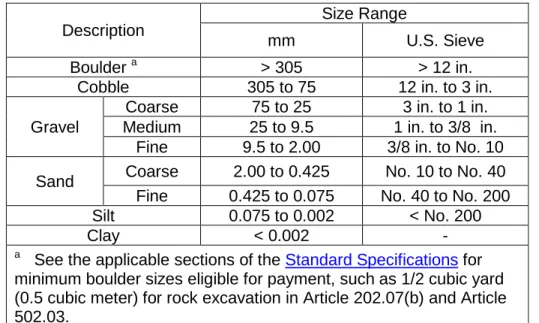
Generally speaking, soil types in Illinois can consist of (from coarsest to finest) boulders, cobbles, gravel, sand, silt, and clay. Table 1 shows the particle size limits for different soil constituents.

Table 1. IDH Particle Size Limits of Soil Constituents defined in AASHTO M 146

Description

Size Range

mm U.S. Sieve

Boulder a > 305 > 12 in.

Cobble 305 to 75 12 in. to 3 in.

Gravel

Coarse 75 to 25 3 in. to 1 in. Medium 25 to 9.5 1 in. to 3/8 in.

Fine 9.5 to 2.00 3/8 in. to No. 10 Sand Coarse 2.00 to 0.425 No. 10 to No. 40 Fine 0.425 to 0.075 No. 40 to No. 200 Silt 0.075 to 0.002 < No. 200

Clay < 0.002 -

a_{See the applicable sections of the}_{Standard Specifications}_for minimum boulder sizes eligible for payment, such as 1/2 cubic yard (0.5 cubic meter) for rock excavation in Article 202.07(b) and Article 502.03.

Soils types are identified not only by their particle size, but by their properties as well. Although accurate identification of soils is normally carried out in the laboratory, the lack of necessary facilities in the field requires the Inspector to make reasonably approximate field identifications. Accordingly, identification and description are based on a combination of experience along with some simple visual and physical identification tests (such as grittiness, cohesiveness, finger pressure, and other sensory assessments). As soil samples are extracted from stockpiles, borings, test pits, or road cuts, they should be approximately identified in the field in terms of texture, color, and engineering classification. For purposes of this course, discussion will pertain to soils comprised of gravel, sand, silt, clay, and organics (generally fine grained). Refer to the Illinois Division of Highways (IDH) Textural Classification Chart in Appendix C for soil types and abbreviations.

Gravel is coarse, cohesionless, and generally exhibits a high friction angle and strength. It may be washed or contain fines.

Sand is easily identifiable by sight and has very little cohesion. Sand does not ribbon between thumb and finger, and rarely holds together when compressed in the hand. Individual grains are easily seen with the naked eye, even when moist. Sandy soils can be classified as sand, sandy loam, or sandy clay loam.

Silt is identifiable by its floury consistency. It has low cohesion, shears easily, and does not ribbon well between thumb and finger. Silt crumbles easily when dry, and bleeds water if vibrated in the hand when wet (dilatancy). Silt in the field is notorious for pumping when wet. If it is too wet, it cannot achieve adequate compaction. Silty soils can be classified as silt, silty loam, or silty clay loam.

(16)

Clay is identified by its high cohesive strength and soapy appearance when smeared with the finger. Clay ribbons very well between thumb and finger, and is extremely difficult to crumble when dry. In a very moist condition, clay becomes very soft and sticky and will display a pitted texture on a broken surface. A fingerprint impression made in clay is well defined. Clayey soils can be classified as clay, clay loam, silty clay, silty clay loam, or sandy clay.

Organic soils, such as peat and muck, are made up of organic matter typically consisting of decomposed plant material accumulated under conditions of excessive moisture, and can generally be fibrous, sedimentary, or woody. When peat is decomposed such that recognition of plant forms is not possible, it is referred to as muck. These organic soils are dark colored in nature and may exhibit the odor of decaying vegetation.

(17)

3. MOISTURE, DENSITY, AND THE STANDARD PROCTOR

Field density and compaction testing is carried out to ensure that subgrades and embankments have been compacted to their required densities. This involves determining the percent compaction of soils in the field based on the in-place soil density. In order to compute the percent compaction, the in-place (field) dry density of the soil must be compared to the Standard Dry Density (SDD), otherwise known as the Proctor Density, that has been established for that soil. The SDD is determined from a moisture-density relationship (Proctor Curve). Compaction testing thus requires both moisture and density testing to be carried out.

3.1 Soil Moisture Content

Moisture content is an important soil property, as it correlates with such engineering properties as shear strength, permeability, compressibility, and unit weight. Soil moisture content (w) is defined as the ratio (expressed in percent) of the weight of water in a specimen to the dry weight of soil grains in the specimen, as given by equation 3-1:

𝑀𝑜𝑖𝑠𝑡𝑢𝑟𝑒

𝐶𝑜𝑛𝑡𝑒𝑛𝑡

,

𝑤

(%) =

_𝑊𝑡𝑊𝑡_._𝑜𝑓.𝑜𝑓_𝐷𝑟𝑦𝑊𝑎𝑡𝑒𝑟_{𝑆𝑜𝑖𝑙}𝑖𝑛_𝑖𝑛𝑆𝑝𝑒𝑐𝑖𝑚𝑒𝑛_{𝑆𝑝𝑒𝑐𝑖𝑚𝑒𝑛}

× 100

3-1 The moisture content test is simple to perform, requiring only a balance and a means of drying the specimen. The test is conducted by weighing a mass of soil while wet and then drying it to obtain a constant dry weight. The difference of the two weights is the weight of water that was present in the sample while wet. Thus, the numerator and denominator of Equation 3-1 can be defined as follows:

𝑊𝑡

.

𝑜𝑓

𝑊𝑎𝑡𝑒𝑟

𝑖𝑛

𝑆𝑝𝑒𝑐𝑖𝑚𝑒𝑛

= (

𝑊𝑒𝑡

𝑆𝑜𝑖𝑙

+

𝑃𝑎𝑛

𝑊𝑡

. )

−

(

𝐷𝑟𝑦

𝑆𝑜𝑖𝑙

+

𝑃𝑎𝑛

𝑊𝑡

. )

3-1a

𝑊𝑡

.

𝑜𝑓

𝐷𝑟𝑦

𝑆𝑜𝑖𝑙

𝑖𝑛

𝑆𝑝𝑒𝑐𝑖𝑚𝑒𝑛

= (

𝐷𝑟𝑦

𝑆𝑜𝑖𝑙

+

𝑃𝑎𝑛

𝑊𝑡

. )

− 𝑃𝑎𝑛

𝑊𝑡

.

3-1b The moisture content test is typically conducted in the laboratory according to Illinois Modified AASHTO T 265, whereby the soil samples are dried in a thermostatically-controlled oven for a minimum of 16 hours. A copy of the test method can be found in the Department’s Manual of Test Procedures for Materials; also see Appendix A for a complete list of Department test procedures.

3.2 Field Moisture Content / Field Soil Drying

The Inspector in the field often does not have access to a thermostatically-controlled drying oven as required by Illinois Modified AASHTO T 265. However, the Inspector may need to quickly obtain an approximate "oven-dry" moisture content in order to perform a nuclear gauge moisture correlation or the One-Point Proctor Test (see Section 4). Thus, any of the following are acceptable for field drying:

• Microwave oven • Hot plate

• Electric heat lamp • Portable grill • Camp stove • Kitchen stove

Refer to Illinois Modified AASHTO T 310 and T 272, as well as ASTM D 4643 for additional information (see Appendix A).

(18)

CLASS PROBLEM 1: Determination of Moisture Content in the Field.

In the field lab, moist samples were weighed in their containers, dried in a microwave, and then subsequently weighed after drying. Complete the table below to determine the moisture content of each sample. Weight of Wet Soil + Container WW (grams) Weight of Dry Soil + Container DW (grams) Weight of Container WC (grams) Weight of Water in Soil WW – DW (grams) Weight of Dry Soil DW – WC (grams) Moisture Content 𝑊𝑊 − 𝐷𝑊 𝐷𝑊 − 𝑊𝐶 × 100 (%) 792 608 102 1129 901 154 669 383 97

Solution Process: Use equations 3-1a, 3-1b, and 3-1.

Note: When the digit next beyond the last place to be retained (or reported) is equal to or greater than 5, increase by 1 the digit in the last place retained (Illinois Modified ASTM E 29). For example, 1.25 rounds to 1.3.

(19)

3.3 Soil Density and the Standard Proctor Test

For Department projects, the moisture-density relationship of soils is obtained via the Standard Proctor Test according to Illinois Modified AASHTO T 99, Method C (refer to the Department’s Manual of Test Procedures for Materials; also see Appendix A for a complete list of Department test procedures). Note that a soil’s moisture content and density are directly related during and after the compaction process.

Based on this moisture-density relationship, greater density almost always results in: • Greater strengths

• Greater stability • Less compressibility

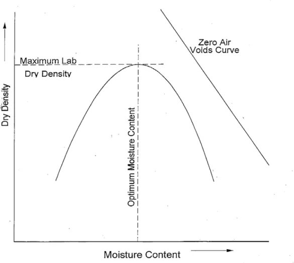
A typical moisture-density relationship for a given soil prepared at a given compactive effort is shown below in Figure 1. This moisture-density relationship, in which dry density is plotted versus moisture content, represents the Proctor Curve:

Figure 1. Proctor Curve showing the relationship between moisture content and dry density.

(20)

The maximum dry density obtained from the Proctor Curve is known as the Standard Dry Density (SDD), or Proctor Density, established for that soil. Furthermore, the soil’s moisture content at which this maximum density occurs is known as the Optimum Moisture Content (OMC). The soil density and the inferred degree of soil strength are influenced by these factors:

1. Moisture content of the soil. As moisture content increases from below optimum, the density and strength increase as the material is compacted. Density and strength will continue to increase under the same compactive effort as the moisture approaches optimum, reaching their peak at the OMC. As moisture exceeds optimum (still under the same compactive effort) the density and strength begin to decrease.

2. Nature of the soil (gradation, chemical, and physical properties). Of primary concern are the gradation, size, shape, and mineralogical composition of the individual particles. Generally, as soils range from poorly graded to well-graded, the maximum density increases. Well-graded soils contain such a wide range of particle sizes that small particles fill the void spaces between large particles, thereby increasing the maximum density. This situation cannot prevail when the aggregate is gap-graded or uniform in size. Whenever void space is replaced with soil grains, the density is increased. The OMC is a function of the soil specific surface (total surface area of particles per volume). Fine grained soils have larger specific surface than coarse grained soils. This explains why clays exhibit higher OMC than sands.

3. Type and amount of compactive effort. In general, as the compactive effort is increased, the maximum density is increased, and the OMC is reduced. The moisture density curve obtained in the laboratory, for a given soil, does not necessarily correspond exactly to the curve that would be obtained in the field, under different compaction conditions. Such field curves, obtained with various rollers at different numbers of passes, do correspond reasonably well with the laboratory curves. Both research and practice indicate that with the proper compaction equipment, no difficulty should be experienced in achieving 95% or more of the laboratory maximum dry density, provided the soil in the field is near the laboratory OMC.

To develop the Proctor Curve, a series of moisture-density data points are generated in the laboratory according to Illinois Modified AASHTO T 99, Method C. The basic process is as follows:

• Each data point represents a soil sample compacted at a particular moisture content in a 1/30 ft3 mold in three approximately equal layers; each layer is compacted 25 times with a 5.5 lb rammer falling 12 inches.

• After the final layer has been compacted and the soil trimmed flush with the top of the mold, the sample is weighed and the wet density is computed.

• Upon compaction, each sample is then oven-dried and its moisture content is computed along with its dry density. Once the dry densities and corresponding moisture contents are recorded, the Proctor moisture-density (compaction) curve can be drawn.

• A minimum of four data points, all at different moisture contents, will need to be plotted in order to draw a best fit curve. Three of the four data points should be ascending on the wet curve (increase in wet density with increase in moisture).

(21)

Equation 3-2 defines wet density (γwet) as follows:

𝑊𝑒𝑡

𝐷𝑒𝑛𝑠𝑖𝑡𝑦

,

γ

_𝑤𝑒𝑡

₌

𝑊𝑡.𝑜𝑓𝑊𝑒𝑡𝑆𝑜𝑖𝑙𝑖𝑛𝑃𝑟𝑜𝑐𝑡𝑜𝑟𝑀𝑜𝑙𝑑

𝑉𝑜𝑙𝑢𝑚𝑒𝑜𝑓𝑃𝑟𝑜𝑐𝑡𝑜𝑟𝑀𝑜𝑙𝑑 3-2 However, for computational purposes, use Equation 3-2a:

γ

_𝑤𝑒𝑡

₌

_𝑊𝑡

_.

_𝑜𝑓

_𝑊𝑒𝑡

_{𝑆𝑜𝑖𝑙}

_𝑖𝑛

_{𝑃𝑟𝑜𝑐𝑡𝑜𝑟}

_{𝑀𝑜𝑙𝑑}

_×

_{𝑀𝑜𝑙𝑑}

_{𝐹𝑎𝑐𝑡𝑜𝑟}

3-2a Where, if using a scale that weighs the mold and soil in pounds, the Mold Factor is calculated as follows:

𝑀𝑜𝑙𝑑

𝐹𝑎𝑐𝑡𝑜𝑟

=

_{𝑉𝑜𝑙𝑢𝑚𝑒}_𝑜𝑓_{𝑃𝑟𝑜𝑐𝑡𝑜𝑟}1 _{𝑀𝑜𝑙𝑑} 3-2b Or, if using a scale that weighs the soil and mold in grams, the Mold Factor requires a unit conversion as follows:

𝑀𝑜𝑙𝑑

𝐹𝑎𝑐𝑡𝑜𝑟

=

_{𝑉𝑜𝑙𝑢𝑚𝑒}_𝑜𝑓_{𝑃𝑟𝑜𝑐𝑡𝑜𝑟}1 _{𝑀𝑜𝑙𝑑}

×

₄₅₄1𝑙𝑏_𝑔 3-2c The Mold Factor is a conversion factor incorporating the volume of the mold and, if needed, the conversion of grams to pounds. That is, based on a mold volume of 1/30 ft3 for a 4 inch diameter mold per Illinois Modified AASHTO T 99, Method C and knowing there are 454 grams in a pound, the mold factor = 0.0661 lb/g-ft3. Check the calibration records for the mold and adjust the mold factor for the actual volume of the mold. Note that the mold factor is also different for Method B or Method D, which use a 6 inch diameter mold with a greater mold volume.

Once the wet density is known, along with the moisture content, the dry density can be determined. Accordingly, dry density (γdry) is defined in Equation 3-3 as follows:

𝐷𝑟𝑦

𝐷𝑒𝑛𝑠𝑖𝑡𝑦

,

γ

_𝑑

₌

γ𝑤𝑒𝑡

(𝑤+100)

× 100

3-3

(22)

CLASS PROBLEM 2: Determine the SDD and OMC of a Soil

CLASS PROBLEM 2: Determine the Standard Dry Density (SDD) and the Optimum Moisture Content (OMC) of a Soil.

Complete the Moisture-Density Worksheet on the next page, and determine the SDD and OMC of a soil.

Solution Process:

1. Calculate moisture content, and wet and dry densities. Complete the third and fourth rows of the worksheet on the next page using equations 3-1a, 3-1b, 3-1, 3-2a, and 3-3.

2. Plot wet and dry densities versus moisture content. Once the moisture-density worksheet is completed, the data from the last three columns will be plotted on the graph provided. Plot Wet Density versus Actual Moisture Content (Wet Curve) and Dry Density versus Actual Moisture Content (Proctor Curve) for all four specimens on the same graph; the density axis is split to accommodate both sets of data.

3. Draw the best fit Wet Curve. Note: At least three points must be ascending.

4. Back-calculate dry points near break. Take two or three wet points from the Wet Curve to back-calculate dry points as additional data in helping to draw the apex of the Proctor Curve. To back-calculate dry points:

a) Choose a moisture content.

b) Find corresponding density on Wet Curve for the moisture content chosen.

c) Calculate the dry densities corresponding to the same moisture contents as follows:

𝐷𝑟𝑦

𝐷𝑒𝑛𝑠𝑖𝑡𝑦

,

γ

_𝑑

₌

𝑊𝑒𝑡𝐷𝑒𝑛𝑠𝑖𝑡𝑦𝑐𝑜𝑟𝑟𝑒𝑠𝑝𝑜𝑛𝑑𝑖𝑛𝑔_{𝐶ℎ𝑜𝑠𝑒𝑛}_{𝑀𝑜𝑖𝑠𝑡𝑢𝑟𝑒}𝑡𝑜𝑎_{𝐶𝑜𝑛𝑡𝑒𝑛𝑡+100}𝑐ℎ𝑜𝑠𝑒𝑛𝑀𝑜𝑖𝑠𝑡𝑢𝑟𝑒𝐶𝑜𝑛𝑡𝑒𝑛𝑡

_{× 100}

5. Plot dry points near break. Plot the back-calculated dry points from Step 4.

6. Draw the best fit Proctor (“Dry”) Curve.

(23)

Step 1. Complete the moisture-density worksheet below.

𝑊𝑡

.

𝑜𝑓

𝑊𝑎𝑡𝑒𝑟

𝑖𝑛

𝑆𝑝𝑒𝑐𝑖𝑚𝑒𝑛

= (

𝑊𝑒𝑡

𝑆𝑜𝑖𝑙

+

𝑃𝑎𝑛

𝑊𝑡

. )

−

(

𝐷𝑟𝑦

𝑆𝑜𝑖𝑙

+

𝑃𝑎𝑛

𝑊𝑡

. )

3-1a

𝑊𝑡

.

𝑜𝑓

𝐷𝑟𝑦

𝑆𝑜𝑖𝑙

𝑖𝑛

𝑆𝑝𝑒𝑐𝑖𝑚𝑒𝑛

= (

𝐷𝑟𝑦

𝑆𝑜𝑖𝑙

+

𝑃𝑎𝑛

𝑊𝑡

. )

− 𝑃𝑎𝑛

𝑊𝑡

.

3-1b

𝑀𝑜𝑖𝑠𝑡𝑢𝑟𝑒

𝐶𝑜𝑛𝑡𝑒𝑛𝑡

,

𝑤

(%) =

_𝑊𝑡𝑊𝑡_._𝑜𝑓.𝑜𝑓_𝐷𝑟𝑦𝑊𝑎𝑡𝑒𝑟_{𝑆𝑜𝑖𝑙}𝑖𝑛_𝑖𝑛𝑆𝑎𝑚𝑝𝑙𝑒_{𝑆𝑎𝑚𝑝𝑙𝑒}

× 100

3-1

𝑊𝑒𝑡

𝐷𝑒𝑛𝑠𝑖𝑡𝑦

,

γ

_𝑤𝑒𝑡

₌

_𝑊𝑡

_.

_𝑜𝑓

_𝑊𝑒𝑡

_{𝑆𝑜𝑖𝑙}

_𝑖𝑛

_{𝑃𝑟𝑜𝑐𝑡𝑜𝑟}

_{𝑀𝑜𝑙𝑑}

_×

_{𝑀𝑜𝑙𝑑}

_{𝐹𝑎𝑐𝑡𝑜𝑟}

3-2a

𝐷𝑟𝑦

𝐷𝑒𝑛𝑠𝑖𝑡𝑦

,

γ

_𝑑

₌

γ𝑤𝑒𝑡 (𝑤+100)

× 100

3-3

Step 2. Plot wet and dry densities versus actual moisture content on the next page.

Step 3. Draw the best fit Wet Curve using the data points plotted in step 2.

Step 4. Take three points from the Wet Curve and back-calculate three dry data points. For example:

Moisture Content Chosen Corresponding Wet Density from Wet Curve

Calculated Dry Density corresponding to chosen Moisture Content 18.0 % 125.6 pcf 106.4 pcf 19.0 % 126.5 pcf 106.3 pcf 17.5 % 124.9 pcf 106.3 pcf

𝐷𝑟𝑦

𝐷𝑒𝑛𝑠𝑖𝑡𝑦

,

γ

_𝑑

₌

𝑊𝑒𝑡

𝐷𝑒𝑛𝑠𝑖𝑡𝑦

𝑐𝑜𝑟𝑟𝑒𝑠𝑝𝑜𝑛𝑑𝑖𝑛𝑔

𝑡𝑜

𝑎

𝑐ℎ𝑜𝑠𝑒𝑛

𝑀𝑜𝑖𝑠𝑡𝑢𝑟𝑒

𝐶𝑜𝑛𝑡𝑒𝑛𝑡

𝐶ℎ𝑜𝑠𝑒𝑛

𝑀𝑜𝑖𝑠𝑡𝑢𝑟𝑒

𝐶𝑜𝑛𝑡𝑒𝑛𝑡

+ 100

× 100

(24)

Step 5. Plot the back-calculated dry points on the graph below.

Step 6. Complete the apex of the Proctor (“Dry”) Curve using the points plotted in step 5.

Step 7. Determine Standard Dry Density (SDD) and Optimum Moisture Content (OMC).

Proctor Density, SDD = __________ Optimum Moisture Content, OMC = __________

De

n

s

it

(25)

4. FAMILY OF CURVES AND THE ONE-POINT PROCTOR

For many types of construction, it is often impractical to perform a complete moisture-density analysis of all the soils encountered. This is particularly true for highway construction because of the great number of different soil types that are encountered. It would be both time consuming and uneconomical to establish a Proctor curve for each new soil type. However, numerical values for the Standard Dry Density and Optimum Moisture Content for each soil is needed for comparison with the in-place field measurements in order to determine if the field compaction and moisture content meet the minimum contract specifications. The SDD and the OMC can approximately be estimated by using the family of curves method outlined in Illinois Modified AASHTO T 272 (see Appendix A).

On projects with a significant quantity of earthwork, the Geotechnical Report may contain a project-specific family of Proctor Curves for excavated material. The Geotechnical Engineer may also develop a project-specific family of curves when a variety of borrow or furnished materials are encountered and may be mixed prior to placement.

A simplified procedure is the one-point Proctor test, in which one density and its corresponding moisture content are determined. The one-point Proctor test can be performed in a field laboratory in a relatively short period of time. The procedure is as follows:

• A soil sample from the field test site is obtained and transported to the field laboratory. • The sample is then compacted in a 4-in. diameter mold, according to Illinois Modified

AASHTO T 99, Method C.

• The mold is struck-off, and the compacted specimen is weighed.

• A portion of the compacted soil sample is then extruded from the mold, weighed, then either oven dried or dried by one of the permissible field methods discussed in Section 3.2, and then re-weighed for moisture content determination.

• The moisture content and the dry density of the compacted sample can then be calculated using Equations 3-1 and 3-3, respectively.

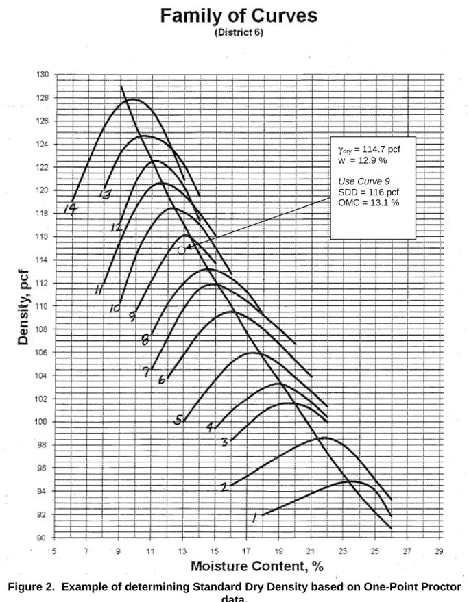
The dry density and moisture content should be plotted on the family of curves (Figure 2). The plotted point should fall on the dry side of the curve. If the point falls on an existing curve, the SDD and OMC defined by that curve should be used. If the point falls between existing curves, the higher curve should be chosen. If the point falls significantly below or above the existing family of curves, or if there is a question regarding the validity of a new curve, contact the Geotechnical Engineer. A complete laboratory moisture-density relationship may be required.

(26)

Figure 2. Example of determining Standard Dry Density based on One-Point Proctor data. γdry = 114.7 pcf w = 12.9 % Use Curve 9 SDD = 116 pcf OMC = 13.1 %

(27)

CLASS PROBLEM 3: Determine the Standard Dry Density (SDD) and Optimum Moisture Content (OMC) of a soil by the One-Point Proctor Test.

CLASS PROBLEM 3: Determine the SDD and OMC by One-Point Proctor

Solution Process: Complete the last five columns of the table below. On the Family of Curves figure below, plot the data point corresponding to the Dry Density and Actual Moisture Content, and choose the appropriate Proctor Curve. Report the SDD and OMC. Compute all values in exactly the same manner as in Class Problem 2.

One-Point Proctor Test Data

Remember: Wet Density = Wet Soil in Mold Weight x Mold Factor = Column 3 x 0.0661

(28)

5. FIELD DENSITY MEASUREMENT AND COMPACTION

Subgrade and embankment soils need to be compacted to a minimum density with an acceptable moisture content.

• SDD is used to determine density acceptability

o Specifications set minimum % Compaction required • OMC is used to determine field moisture acceptability

o Specifications set maximum % of OMC required

Density can be measured in the field by either the Nuclear Gauge or by the Sand Cone Test. Moisture is measured as previously discussed in Section 3.

5.1 Nuclear Gauge Testing

The field dry density is determined by the nuclear gauge method according to Illinois Modified AASHTO T 310 (see Appendix A) using the direct transmission procedure. In this procedure, the total or wet density is determined by the attenuation of gamma radiation where a source is placed at a known depth up to 12 inches, while the detector remains at the surface. With appropriate gauge calibration and adjustment of data, the wet density is determined. The moisture content of the in situ soil is also determined by the nuclear gauge using the backscatter procedure. In this procedure, the thermalization or slowing of fast neutrons is measured with both the neutron source and the thermal neutron detector at the surface. The dry density is then computed from the wet density, using Equation 3-3. Figure 3 shows the test gauge performing both procedures.

Figure 3. Nuclear Gauge Test Illustrating Direct Transmission and Backscatter Procedures.

The moisture content measured by the gauge frequently differs from that determined by “oven-drying” a soil sample from directly beneath the gauge test location. This difference is due to the chemical composition of the sample. Hydrogen in forms other than water and carbon will cause nuclear gauge measurements in excess of the true value. Examples are road oil and asphalt. Chemically bound water, such as found in gypsum, will also cause measurements in excess of the true value. Some chemical elements such as boron, chlorine, and minute quantities of cadmium will cause measurements lower than the true value. Soils containing iron or iron oxides, having a higher capture cross section (absorption of neutrons), will cause measurements lower than the true value. Refer to Illinois Modified AASHTO T 310 for sampling soil at the test location to determine the “oven-dried” moisture and adjusting the gauge test results to determine the dry density and percent compaction.

(29)

5.2 Sand-Cone Testing

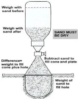
The sand cone method is sometimes used when a nuclear gauge is not available. The general procedure involves excavating a hole in the material to be tested and filling the void with an equal volume of sand using the apparatus shown in Figure 4. Thus, the exact volume of soil removed can be determined. Upon weighing the entire contents of the excavated material along with knowing the exact volume of material removed, a wet density can then be calculated. Furthermore, once a field moisture test is performed on the wet material, the dry density is computed. The specific procedure for this test can be found in Illinois Modified AASHTO T 191 (see Appendix A).

Figure 4. Sand Cone Test Apparatus.

5.3 Compaction and Moisture Acceptance

Percent compaction and percent of optimum moisture in the field are determined by the following equations:

%

𝐶𝑜𝑚𝑝𝑎𝑐𝑡𝑖𝑜𝑛

=

𝐹𝑖𝑒𝑙𝑑𝐷𝑟𝑦_𝑆𝐷𝐷𝐷𝑒𝑛𝑠𝑖𝑡𝑦

× 100

5-1

(30)

CLASS PROBLEM 4: Determination of Percent Compaction and Percent of Optimum Moisture.

Complete the worksheet below to determine the percent compaction and percent of optimum for each of the three cases.

Solution Process: Use equations 5-1 and 5-2.

In-Place Field Dry Density (pcf) In-Place Field Moisture Content (%) Standard Dry Density (pcf) Optimum Moisture Content (%) Percent Compaction (%) Percent of Optimum (%) 100.3 11 108.0 12 108.2 14 111.6 16 101.2 16 94.0 13

(31)

6. FIELD SOIL STABILITY AND STRENGTH TESTING 6.1 Dynamic Cone Penetrometer (DCP) Testing

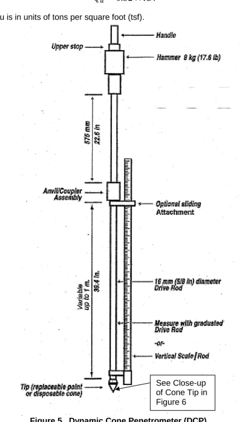
The Dynamic Cone Penetrometer, or DCP (Illinois Test Procedure 501, see Appendix A), is primarily used to determine the immediate bearing value (IBV) of treated or untreated subgrade. The IBV is used to evaluate subgrade stability and determine the depth of subgrade treatment. The DCP is also used to determine the unconfined compressive strength (Qu) of foundation bearing soils.

The DCP consists of a graduated stainless steel rod approximately 40 inches long with a cone attached to one end and an anvil attached to the other. A sliding hammer, weighing 17.6 lbs, is used to drive the instrument into the ground by dropping 22.6 inches. The DCP assembly and its components are shown in Figure 5.

Testing involves driving the cone into the material to be tested and recording the number of blows for every 6 inches of penetration. After the cone has been seated and an initial reading is taken, the number of blows is recorded for each interval of 6 inches penetrated. (Note that the cone may not be driven in exact 6 inch increments every time and may exceed 6 inches upon the last blow for that interval.) The test is repeated to a total depth of at least 18 inches and up to 36 inches. Knowing the number of blows per each 6 inch interval along with the net amount of penetration within the interval (depth is cumulatively recorded), a penetration rate for each interval can be calculated. Once the penetration rate, or “Rate”, within each interval is known, then the IBV can be easily determined for each interval.

The Dynamic Cone Penetration Test worksheet (BMPR SL30 form) may be used to record and calculate data. The worksheet is included in Appendix C-2. An example from the worksheet is as follows:

Test Location and Remarks Initial Depth A B C D E STA 12+00, 4 in. Depth 10 16 22 28 34 O/S 8 ft RT Blows 1 3 4 7 10

Wet SiC Rate 6 2 1.5 0.9 0.6

Cut/Fill Transition IBV <1 3 4 8 14

Qu

Initial Depth = Depth of the DCP cone tip at or below the existing ground surface. Depth = Cumulative depth in inches.

Blows = The number of blows per depth increment (i.e., 6-in. interval).

Rate = Inches of penetration per blow. For example, the Rate in column “A” equals the Depth (10 in.) minus the Initial Depth (4 in.), that quantity (6 in.) divided by number of Blows (1). The Rate in column “C” equals the Depth (22 in.) minus the Depth in column “B” (16 in.), that quantity divided by number of Blows (4).

Once the Rate has been calculated, the IBV can be determined in a couple of ways. Firstly, it may be directly obtained from Equation 6-1:

𝐼𝐵𝑉

= 10

(0.84−1.26×log[𝑅𝑎𝑡𝑒]) _6-1

(32)

Secondly, the IBV may be determined more easily by using Table 2 (interpolation may be needed). After determining the IBV, then a Qu strength can be correlated from the IBV using Equation 6-2. Table 2 also includes the Qu correlation.

𝑄

𝑢

= 0.32 ×

𝐼𝐵𝑉

6-2

Where, Qu is in units of tons per square foot (tsf).

Figure 5. Dynamic Cone Penetrometer (DCP). See Close-up of Cone Tip in Figure 6

(33)

Figure 6. Detail of cone tip of the Dynamic Cone Penetrometer (DCP).

Table 2. Correlation between DCP Penetration Rate, IBV, and Qu.

Rate (in./blow) IBV Qu (tsf) 0.5 17 5.4 0.7 11 3.5 0.8 9 2.9 0.9 8 2.6 1.0 7 2.2 1.1 6 1.9 1.3 5 1.6 1.5 4 1.3 2.0 3 1.0 2.6 2 0.6 3.3 1.5 0.5 4.6 1 0.3 > 4.6 < 1 < 0.3

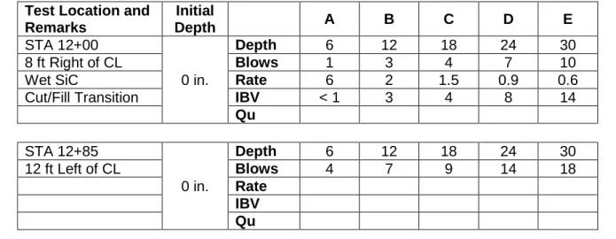
CLASS PROBLEM 5: Determination of IBV using DCP Data.

CLASS PROBLEM 5: Determination of Immediate Bearing Value (IBV) using Dynamic Cone Penetrometer (DCP) Data. Complete the portion of the DCP worksheet shown below for Station 12+85 to find the IBV for each interval.

Solution Process: Calculate the Rate for each interval as discussed above in Section 6.1. Once the Rates are known, find the corresponding IBV and Qu values using Table 2 or Equations 6-1 and 6-2.

Test Location and Remarks Initial Depth A B C D E STA 12+00 0 in. Depth 6 12 18 24 30 8 ft Right of CL Blows 1 3 4 7 10

Wet SiC Rate 6 2 1.5 0.9 0.6

Cut/Fill Transition IBV < 1 3 4 8 14

Qu STA 12+85 0 in. Depth 6 12 18 24 30 12 ft Left of CL Blows 4 7 9 14 18 Rate IBV Qu

(34)

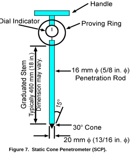
6.2 Static Cone Penetrometer (SCP) Testing

The Static Cone Penetrometer (SCP) (Illinois Test Procedure 502, see Appendix A), is primarily used to determine the IBV of unstable, untreated subgrades.

The SCP consists of a graduated stainless steel rod 18 in. long with a cone attached to one end and a proving ring and handle with a dial gauge attached to the other. The rod is usually graduated in 1-inch to 6-inch intervals. The SCP is shown in Figure 7.

The dial gauge directly reads in units of pounds per square-inch (psi) (not expressed) typically ranging between 0 and 300 psi, though sometimes higher. This dial reading is known as the Cone Index (CI) and is used to compute the IBV. Check the calibration records. The dial reading may require an adjustment from a correlation chart or graph in the calibration records.

Figure 7. Static Cone Penetrometer (SCP).

The IBV may be determined using Table 3 or directly obtained from Equation 6-3:

𝐼𝐵𝑉

=

₄₀𝐶𝐼 6-3

Where CI is the Cone Index (psi), read directly from the dial gauge. The Static Cone Penetration Test worksheet (BMPR SL31 form) is included in Appendix C-3 and is used to record and calculate data.

(35)

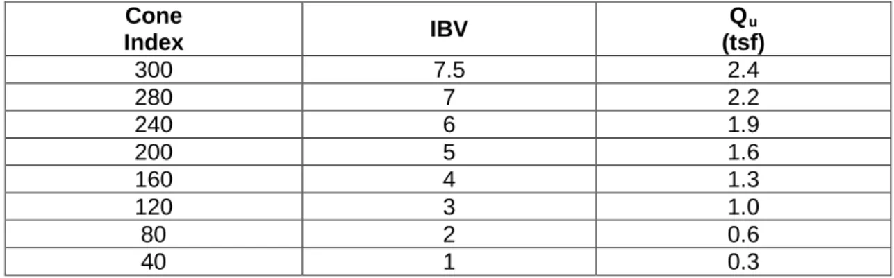
The IBV is correlated to the Qu the same as with the DCP using Equation 6-2. Thus, one can use the DCP or SCP to verify soil unconfined compressive strengths in the field. Table 3 shows the correlation between Cone Index (CI), IBV, and Qu.

Table 3. Correlation between Cone Index, IBV, and Qu.

Cone Index IBV Qu (tsf) 300 7.5 2.4 280 7 2.2 240 6 1.9 200 5 1.6 160 4 1.3 120 3 1.0 80 2 0.6 40 1 0.3

6.3 Pocket Penetrometer (PP) Testing

A commonly used approximation of the unconfined compression test can be performed using a hand-size calibrated penetration device called a pocket, or hand, penetrometer. Although the pocket penetrometer test can be used to estimate the strength of cohesive soils, it should only be used as a reconnaissance tool and not as an accurate means of verifying soil strength in the field. The device, which consists of a calibrated spring and a 0.25 inch diameter piston encased inside a metal casing, is shown in Figure 8.

Figure 8. Pocket Penetrometer.

When the piston is pressed, by hand, at a constant rate to penetrate 0.25 inch (the etched line on the piston) into the soil, the calibrated spring is compressed into the penetrometer, giving an unconfined compression strength (Qu)reading on a scale. The extremely small area of the piston, the skill of the operator, and the particular spot on the sample where the piston is applied influence the strength value obtained. Thus, several penetrometer readings may need to be taken and judgment applied to their results in order to better estimate strength.

(36)

PART B: Field Inspection

7. SUBGRADE INSPECTION

The subgrade is defined in Article 101.47 of the Standard Specifications as the “top surface” of a roadbed upon which the pavement and shoulders are constructed. However, the Geotechnical Manual more accurately defines it as the “top 2 feet” of roadbed.

Subgrades may be encountered in a cut section, at-grade or in an embankment fill section as shown below.

Subgrade inspection includes the following: • Subgrade performance requirements • Treatment types

• Identifying subgrade problems • Determining treatment thickness

Top



---

Pavement & Shoulder Structure

-

---



Roadbed Soils

Top 2

ft.

Top Surface

(37)

7.1 Subgrade Performance Requirements

Subgrade inspection is necessary to meet the following performance requirements: • Prevent excessive rutting and shoving during construction;

• Provide uniform support for placement and compaction of pavement layers • Minimize impacts of excessive volume change and frost

• Limit pavement resilient (i.e., rebound) deflections to acceptable limits • Restrict permanent deformation leading to dips in the pavement

Article 301.04 of the Standard Specifications specifies several requirements including: • Subgrades shall be compacted to have a dry density > 95% SDD

• Subgrades shall be compacted to have an immediate bearing value (IBV) > 8.0 • Subgrades shall have construction traffic rutting < ½ in.

• Subgrades in cut sections shall be constructed as follows:

o Cut plan ditches at least to grade ≥ 2 weeks prior to disking

o Disk subgrade 8 in. deep 3 consecutive dry workdays and allow to dry

o Recompact to required density & IBV stability requirements

Most Illinois soils do not provide adequate stability for construction of the overlying pavement, even after disking, drying, and compacting to the required density. Therefore, an Improved Subgrade layer is usually indicated on the plans. An Improved Subgrade is a subgrade modified to meet the performance requirements mentioned above. The following chart illustrates how to establish treatment thickness for Improved Subgrades.

(38)

By policy, on state routes, a minimum of 12 inches of Improved Subgrade is required regardless of the native soil IBV. This policy assumes that, typically, the native soil does not have adequate stability (i.e., IBV ≥ 8). However, there have been occasions when the in-place soil has an IBV greater than 8 and the soil type is high quality. If this situation is encountered, notify the Field Engineer, Geotechnical Engineer, or the Resident Engineer (RE) to determine if an Improved Subgrade may be reduced in thickness. For all other locations, in order for the 12 inch thickness to be adequate, an IBV of 3 or more must be present below the Improved Subgrade as shown in the following figure.

7.2 Treatment Types

An Improved Subgrade is constructed to provide a stable base for the pavement construction and mitigate problem areas in the subgrade. The Improved Subgrade typically consists of a 12 inch layer of chemically modified soil or an aggregate. Soil modification is usually used in rural areas, and aggregate is usually used in urban areas or on small sections. With the exception of recycled concrete, consult the Geotechnical Engineer prior to incorporating recycled or reclaimed materials into the subgrade.

(39)

The plans should include corrective actions for locations where the typical 12 inch Improved Subgrade is not adequate or where unsuitable materials are identified. These corrective actions could include: deeper soil modification, if feasible; removal and replacement with aggregate; removal and replacement with unrestricted soil; using geosynthetics in conjunction with aggregate; or some combination of options. The most common remedial action is the removal and replacement with aggregate, particularly when the soil is silty. A geosynthetic may be used to reduce the thickness of aggregate needed; however, geosynthetics are most effective for soils with very low IBVs.

7.2.1 Soil Modification

Chemically modifying subgrade soils is the most economical method for improving subgrade soils. It is most frequently used in rural areas because the operation can be very dusty. Soils may be chemically modified by mixing with a variety of materials including cement, lime, fly ash, or bituminous materials. The selection of the type of chemical modifier varies by the soil properties. The most common modifier is a by-product of quicklime by-production called lime kiln dust (Article 1012.03). Successful lime modification mainly depends on the following five factors:

1. The subgrade soil has a minimum clay content of 15%, per Article 1009.01 of the Standard Specifications. On cut or at-grade sections, the plans will indicate alternative treatments for areas not meeting this requirement. The limits shown on the plans are approximate and should be confirmed by the Inspector. For embankment sections, a special provision outlining the requirements for embankment soil should be included in the contract. The requirements should also specify the clay content limit for the top two feet of the embankment.

2. The subgrade soil beneath the lime modified layer must have a minimum IBV of 3. At lower bearing values, additional remedial action may be necessary. 3. The lime kiln dust must be distributed uniformly over the area to be modified. 4. The lime kiln dust must be homogeneously processed. There should be no

large clumps of soil or pockets of lime following processing.

5. A sufficient amount of water must be present for the lime-soil reaction to take place. The quantity of water shown on the plans is an estimate. The amount of water needed depends on the field conditions at the time of modification. Having too much water is not as big a concern as not having enough. A quick check for adequate moisture can be made by picking up a handful of material immediately behind the processor and squeezing it. If it crumbles easily, more water needs to be added. The moisture content is probably adequate if, after squeezing, the material can be manipulated without crumbling.

Mix designs are not typically developed prior to construction because the source of lime is not known until the contractor identifies one for sampling. Soil samples and lime samples shall be submitted for mix design at least 45 days prior to construction according to Article 302.04 of the standard specifications.

For situations where the soil does not contain 15% clay or a lime design is not available for the subgrade soil, contact the Geotechnical Engineer for assistance. For Project Procedures Guide sampling requirements, refer to Appendix B.

(40)

For the other materials available that can be effective for subgrade modification, the two primary alternatives are slag cement and Class C fly ash. These materials would generally be used where the subgrade soil has a clay content less than 15% and subgrade replacement with aggregate would be cost prohibitive. Section 302 of the Standard Specifications addresses soil modification with lime and other alternative materials. If subgrade modification is proposed during design, the plans will indicate the limits of treatment and include a Special Provision describing the method of construction. If a Contractor proposes subgrade modification, in lieu of aggregate required on the plans, contact the Geotechnical Engineer.

7.2.2 Granular Improved Subgrades

The project plans may call for a granular improved subgrade through a variety of pay items and thicknesses. The most common pay items include Subbase Granular Material (Type A or B) and Aggregate Base Course (Type A or B). Each pay item allows for use of specific course aggregate gradations. Where the gradation CA 6 is used, the thickness should not exceed 9 to 12 inches (depending on the locally available materials) as it may become internally unstable, particularly with rounded natural gravels.

7.2.3 Removal and Replacement

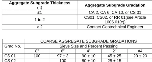
Subgrade treatment requiring thicknesses greater than 12 inches are common where it is necessary to remove the unsuitable/untreatable soil and replacing it. Removal and replacement is the most common type of treatment in silty soils. Replacement materials may be an unrestricted soil or an aggregate. When aggregate is used for replacement, it is common to use Aggregate Subgrade Improvement. In the absence of a Special Provision, the Aggregate Subgrade Improvement should be according to gradations recommended in Table 4 as defined in the BDE Special Provision for Aggregate Subgrade Improvement. The Aggregate Subgrade Improvement is typically capped with 3 inches of CA 6, CA 10, or RAP, unless otherwise specified. RAP may only be used as capping aggregate in the top 3 in. (75 mm) when

aggregate gradations CS 01, CS 02, or RR 01 are used in lower lifts; and it must have 100 percent passing the 1 1/2 in. (37.5 mm) sieve, be well graded, and follow the current Bureau of Materials and Physical Research Policy Memorandum, “Reclaimed Asphalt Pavement (RAP) for Aggregate Applications”. Some Districts may specify a CA 7 or CA 11 capping material as well.

Table 4. Aggregate Subgrade Gradations.

Aggregate Subgrade Thickness

(ft) Aggregate Subgrade Gradation

≤1 CA 2, CA 6, CA 10, or CS 01

1 to 2 CS01, CS02, or RR 01(see Article 1005.01(c))

> 2 Contact Geotechnical Engineer

COARSE AGGREGATE SUBGRADE GRADATIONS Grad No. Sieve Size and Percent Passing

8” 6” 4” 2” #4

CS 01 100 97 ± 3 90 ± 10 45 ± 25 20 ± 20

(41)

7.3 Identifying Subgrade Problems

Subgrade problems can include the presence of unsuitable materials or locations where the typical 12 inch Improved Subgrade does not provide adequate support. The plans should indicate areas requiring additional subgrade treatment that were identified in the projects geotechnical report. Limits of these areas are approximate and must be evaluated in the field by the Inspector. The Inspector should visually verify that the soil in the field is consistent with the soil described in the project’s geotechnical report for subgrade areas needing treatment.

Problems with unsuitable or unstable materials usually occur in cuts or at-grade. Subgrade stability problems may also occur on shallow embankments when the embankment is placed on unstable material. Subgrade soils should consist of unrestricted materials; with the exception of granular soils, materials classified as restricted in Table 7 are considered unsuitable subgrade soils. Granular soils usually require confinement with larger aggregate (e.g., CA 6) to achieve stability under construction traffic.

The Inspector must visually observe the performance of the subgrade prior to treatment. If one or more of the conditions below is encountered, the routine 12 inch Improved Subgrade may not provide adequate stability:

1. The untreated subgrade in cut or at-grade sections is wet and will not achieve density after following the steps outlined in Article 301.04.

2. The untreated subgrade ruts more than 2 inches under heavy equipment (field tests have shown that subgrades with IBV of 3 give an average rut depth of 2 in.). 3. The untreated subgrade pumps or rolls under heavy equipment.

Proof rolling refers to driving a loaded truck or heavy construction equipment over the subgrade and observing rutting or pumping (Figure 9). In some cases, proof rolling may be specifically included in the contract as a Special Provision. In general, the Inspector should always observe the performance of the subgrade during construction. Prior to Improved Subgrade construction, the subgrade is often used as a haul road unless prohibited by Special Provision. This gives field personnel a good opportunity to check subgrade conditions. Also, excessive moisture could have adverse effects on the density and stability (IBV) of both clayey and silty soils; however, its effect is more significant on silty soils as shown in Figure 10. Note that for silts, the IBV drops dramatically past optimum, whereas for clays, the decrease is more gradual.

Sand Silt Clay

Visually verify that soils described in the Geotechnical

Report are consistent with the field soils.

(42)

Figure 9. Rutting and pumping under proof rolling or construction traffic.

The in-place IBV of unstable subgrades should be determined using a cone penetrometer; either the SCP or the DCP. The IBV data is used to measure the in-place stability of the subgrade and determine the extent of any remedial action required. When obtained in the field using a DCP or SCP, the IBV is considered equivalent to the field California Bearing Ratio (CBR) test (ASTM D 4429). When evaluating the suitability of subgrade improvement, the IBV data directly below the estimated depth of subgrade improvement should be used. In general, the IBV data between a depth of 12 and 30 inches should be used to evaluate the adequacy of a 12 inch Improved Subgrade.

Figure 10. Effect of Moisture Content on IBV. Rutting Under

Loaded Construction Traffic?

(43)

In addition to conducting tests, the subgrade soil should be described as per Section 2. The DCP or SCP may not provide an accurate measure of IBV in silty soils. Silty soils must be “proof rolled” using construction equipment immediately prior to testing. Proof rolling commonly locates moisture sensitive soils. Silty soils must be identified in the field, not only for stability, but also to determine their frost susceptibility. The frost penetration depth varies from 4 feet in the northern third of the state to 2 feet in the southern third of the state. The Department uses three criteria according to the Geotechnical Manual to determine if a soil is frost susceptible:

1. The level of capillary rise is within the depth of frost penetration.

2. The soil contains ≥ 65% silt and fine sand determined by AASHTO T 88. 3. The plasticity index (PI) is less than 12.

Upon identifying a silty soil in the field, the Inspector should typically recommend removal of the soil and replacement with unrestricted materials or suitable aggregate. Frost susceptible conditions are commonly found in shallow cuts or at-grade sections.

7.4 Determining Treatment Thickness

The depth of treatment should be based on the DCP or SCP test data and may also depend on the thickness of any unsuitable or frost susceptible material. Unsuitable materials should be removed to a depth of 2 feet below the top of proposed subgrade. Frost susceptible materials should be removed to a depth equal to the frost penetration depth at that location. For unstable materials, the total thickness of improved subgrade required for different IBVs is shown in Table 5. Furthermore, guidelines for aggregate thickness reductions using geosynthetics is shown in Table 6.

Table 5. Improved Subgrade Thickness Requirements.

DCP (in./blow) SCP (psi) IBV* Improved Subgrade Thickness (in.) < 2 > 120 > 3 12 2.8 80 2 18 4.6 40 1 24 > 4.6 < 40 < 1 (Contact Geotechnical Engineer) n/a

*IBV of the subgrade beneath the assumed improved layer.

Table 6. Guideline for Aggregate Thickness Reduction Using Geosynthetics.

IBV / CI Aggregate Cover without Geosynthetics in. (mm) Aggregate Cover with Geosynthetics in. (mm) Aggregate Cover with Geogrid in. (mm) 1 / 40 22 (560) 16 (450) 15 (375) 1.5 / 60 18 (450) 12 (300) 12 (300) 2 / 80 16 (400) 12 (300) 10 (250) 3 / 120 12 (300) 12 (300) 9 (230)

(44)

If the penetration rate of the DCP is greater than 6 inches per blow (IBV < 0.7), the required thickness of Improved Subgrade exceeds 24 inches. In these cases, the Geotechnical Engineer must be contacted to better evaluate the field conditions.

In addition to Table 5, Figure 11 showsthickness design as a function of IBV, Cone Index (CI), Shear Strength, and unconfined compressive strength (Qu) for subgrade treatment (using granular backfill or modified soil). Inspectors are advised to understand how to use the figure, as well as have a copy of it available with them in the field to be readily used. In order to not cause construction delays, it is very important that the Inspector becomes familiar with the method/procedure of determining the treatment thickness in the field, especially when more frequent testing is needed. To fully understand the process, a class problem has been prepared with four different scenarios, in which the first has been completed as an example.

IBV 1 2 3 4 5 6 7 8 9

Cone Index (CI) 40 80 120 160 200 240 280 320 360

Shear Strength (psi) 2.25 4.50 6.75 9.00 11.25 13.50 15.75 18.00 20.25 Qu (tsf) 0.32 0.64 1.00 1.28 1.60 1.94 2.24 2.56 2.88 Rate (in./blow) 4.6 2.6 2.0 1.5 1.3 1.1 1.0 0.9 0.8 Rate (blows/6 in.) 1.3 2.3 3.0 4.0 4.6 5.5 6.0 6.7 7.5

Treatment

Thickness (in.) 22.5 15.5 12.5 11 9.5 8.5 8 7.5 0 Figure 11. Thickness design as a function of IBV, Cone Index (CI), Shear Strength, and

(45)

CLASS PROBLEM 6: Determine Required Subgrade Treatment Thickness

CLASS PROBLEM 6: Determine the required subgrade treatment thickness for the four scenarios shown in the table on page 37. The first scenario has been done for you.

Solution Process: For each of the four scenarios, follow these steps:

1. The contractor completes rough grading. The rough grade is the surface of the untreated subgrade. Then, when plans call for an untreated subgrade or a granular layer(s), prepare the rough graded soil subgrade according to Article 301.04 of the Standard Specifications by disking, drying, and compacting. Then, perform steps 2 thru 7 below. When plans call for Soil Modification, perform steps 2 thru 7 below in suspected weak spots prior to soil modification and adjust the thickness in those localized areas. Perform the soil modification and repeat steps 2 thru 7 below to verify and remediate as needed. 2. Conduct proof rolling and DCP (or SCP) testing at representative locations (preferably

rut locations). Identify the length(s) and width(s) including stations and offsets of any weak subgrades locations requiring further treatment.

3. Determine the IBV (or CI) at the following depth intervals: a. 0 – 6 in.

b. 6 – 12 in. c. 12 – 18 in. d. 18 – 24 in. e. 24 – 30 in.

4. Check IBV (or CI) within 18 inches below the bottom of the Improved Subgrade. The following Case 1 and Case 2 illustrate rough graded subgrade in cut, at-grade, and fill conditions for aggregate, modified soil, and untreated conditions:

(46)

Case 2—Modified or Untreated Subgrade

5. Use Figure 11 to determine the required treatment thickness based on IBV (or CI) for each depth interval. Call this “Required Cover”. Record this in the table on Page 37. 6. Compare this “Required Cover” with the “Available Cover”. “Available Cover” is the

Depth Interval Increment plus 12 inches, assuming an Improved Subgrade plan thickness of 12 inches. Determine the amount of Additional Cover Required.

7. Determine the Total Required Treatment Thickness. The total required treatment thickness is equal to any additional cover required plus the already treated 12 inches of Improved Subgrade.

SCENARIO 1:

Steps 1 – 3: Completed per above.

Step 4: See the IBV (or CI) test results within 18 inches below the bottom of Improved Subgrade, which are recorded under the column “Observed IBV” in the table on Page 37. The IBV and CI values are given as follows:

Depth

(in.) IBV / CI 0 – 6 3 / 120 6 – 12 2 / 80 12 – 18 1 / 40

Step 5: Using Figure 11, determine the “Required Cover” for each depth interval and record it under the column “Required Cover” in the table on Page 37.

(47)

IBV 1 2 3 4 5 6 7 8 9

Cone Index (CI) 40 80 120 160 200 240 280 320 360

Shear Strength (psi) 2.3 4.5 6.75 9.0 11.3 13.5 15.8 18.0 20.3 Qu (tsf) 0.3 0.6 1.0 1.3 1.6 1.9 2.2 2.6 2.9 Rate (in./blow) 4.6 2.6 2.0 1.5 1.3 1.1 1.0 0.9 0.8 Rate (blows/6 in.) 1.3 2.3 3.0 4.0 4.6 5.5 6.0 6.7 7.5

Treatment

Thickness (in.) 23 16 12 11 10 9 8 7 0

Step 6: Compare the “Required Cover” with the “Available Cover” and determine if any additional cover will be required. Note that the “Available Cover” has already been recorded in the table on Page 37. The amounts of Available Cover are as follows:

Depth (in.) Depth Interval Increment (in.) Available Cover (in.) 0 – 6 0 12 + 0 = 12 6 – 12 6 12 + 6 = 18 12 – 18 12 12 + 12 = 24

Tabulate the values for Available Cover and Required Cover, and determine the amount of Additional Cover Required.

Depth (in.) Available Cover (in.) Required Cover (in.) Additional Cover Required (in.) 0 – 6 12 12 0 6 – 12 18 16 0 12 – 18 24 23 0

Since in Scenario 1 the Available Cover is greater than or equal to the Required Cover at each depth interval, no additional cover is required.

(48)

Step 7: Determine Total Required Treatment Thickness. The total required treatment thickness is equal to any additional cover required plus the already treated 12 in. of Improved Subgrade.

Thus, for Scenario 1, the Total Required Treatment Thickness = 0 + 0 + 0 + 12 = 12 in.

Specific Task Training Program Course S-33 Soils Field Testing and Inspection: Course Reference Manual

Specific Task Training Program

Course S-33

Soils Field Testing and Inspection:

Course Reference Manual

Specific Task Training Program

Course S 33

Soils Field Testing and Inspection

Course Reference Manual

Prepared and Published by

Illinois Department of Transportation

Bureau of Materials and Physical Research

Springfield, Illinois

DOCUMENT CONTROL

COURSE REQUIREMENTS FOR

SUCCESSFUL COMPLETION

TABLE OF CONTENTS

List of Figures

List of Tables

PART A: SOILS FIELD TESTING

𝑀𝑜𝑖𝑠𝑡𝑢𝑟𝑒

𝐶𝑜𝑛𝑡𝑒𝑛𝑡

,

𝑤

(%) =

× 100

𝑊𝑡

.

𝑜𝑓

𝑊𝑎𝑡𝑒𝑟

𝑖𝑛

𝑆𝑝𝑒𝑐𝑖𝑚𝑒𝑛

= (

𝑊𝑒𝑡

𝑆𝑜𝑖𝑙

+

𝑃𝑎𝑛

𝑊𝑡

. )

−

(

𝐷𝑟𝑦

𝑆𝑜𝑖𝑙

+

𝑃𝑎𝑛

𝑊𝑡

. )

𝑊𝑡

.

𝑜𝑓

𝐷𝑟𝑦

𝑆𝑜𝑖𝑙

𝑖𝑛

𝑆𝑝𝑒𝑐𝑖𝑚𝑒𝑛

= (

𝐷𝑟𝑦

𝑆𝑜𝑖𝑙

+

𝑃𝑎𝑛

𝑊𝑡

. )

− 𝑃𝑎𝑛

𝑊𝑡

.

𝑊𝑒𝑡

𝐷𝑒𝑛𝑠𝑖𝑡𝑦

,

γ

=

γ

=

𝑊𝑡

.

𝑜𝑓

𝑊𝑒𝑡

𝑆𝑜𝑖𝑙

𝑖𝑛

𝑃𝑟𝑜𝑐𝑡𝑜𝑟

𝑀𝑜𝑙𝑑

×

₌

₌

_𝑊𝑡

_.

_𝑜𝑓

_𝑊𝑒𝑡

_{𝑆𝑜𝑖𝑙}

_𝑖𝑛

_{𝑃𝑟𝑜𝑐𝑡𝑜𝑟}

_{𝑀𝑜𝑙𝑑}

_×

_{𝑀𝑜𝑙𝑑}

_{𝐹𝑎𝑐𝑡𝑜𝑟}

₌

₌

_{× 100}

₌