Institute of Energy Technology, 9 th Semester Report. Control of a variable speed variable pitch wind turbine with full scale power converter

(1)

Institute of Energy Technology ,

9

th

Semester Report

Control of a variable speed

variable pitch wind turbine with

full scale power converter

(2)

(3)

Institute of Energy Technology Pontoppidanstræde 101 Telephone 96 35 92 40 Fax 98 15 14 11 http://www.iet.aau.dk Title:

Control of a variable speed variable pitch wind turbine with full power converter

Theme of PED9:

Design-oriented Analysis of Electric Machines and Power Electronic Sys-tems

Project period:

7.September - 17.December 2007

Project group number: 915 Participants: Massimo Valentini Thordur Ofeigsson Alin Raducu Supervisor: Florin Iov Number of copies: 5 Number of pages:93 Finished:17. December 2007 Synopsis:

This project deals with the control of a small variable speed variable pitch wind turbine with full scale power converter. The chosen wind turbine (WT) concept is, at the moment, the second most common topology in the wind power industry. However it has the chance in the next future to become the best solution as the higher cost is balanced by the power quality, harmonic compensation and full grid support.

In order to optimize the energy capture, a speed control system is required to control the induction generator (IG) rotor speed. The ref-erence speed is obtained by implementing a Maximum Power Point Tracker (MPPT) al-gorithm; the Perturb and Observe method is selected and designed. The speed control of the electric generator is achieved by control-ling the generator side converter using the Di-rect Field Oriented Control (DFOC) which is designed using a step-by-step procedure. When the available wind power exceeds the generator rated power, the wind turbine is operated in power limitation mode with vari-able pitch angle; the pitch control with pro-portional controller is designed and simu-lated. Moreover the switch control between the variable-speed operation and the power limitation mode is designed.

The entire system is simulated using Mat-lab/Simulink, implemented in a dSPACE plat-form and tested with an experimental test setup. A Graphical User Interface (GUI) is built for the real-time evaluation of the control performance. Experimental results succesfully validate the control system design.

(4)

(5)

Preface

The present project report entitledControl of a variable speed variable pitch wind turbine with full

scale power converter is documented by group PED9-915 in 9th semester at Institute of Energy

Technology, Aalborg University. The project period is from 7th September to 17thDecember 2007.

Literature references are mentioned in square brackets by numbers. Detailed information about literature is presented in Bibliography. Appendices are assigned with letters and are arranged in

alphabetical order. Equations are numbered in format (X.Y) and figures are numbered in format

Fig.X.Y, whereX is the chapter number andY is the number of the item. The enclosed CD-ROM

contains the project report in Latex and Adobe PDF formats, documentations used throughout the report and Simulink Models.

Authors would like to thank the supervisor Florin Iov for the support and ideas provided throughout the project period.

The report is conducted by:

Massimo Valentini Thordur Ofeigsson

(6)

(7)

CONTENTS

Part I:

Project Defintion

Part I: Project Defintion 1

1 Introduction 2

1.1 Background to Wind Energy Technology . . . 2

1.1.1 Speed control capability . . . 2

1.1.2 Power control capability . . . 3

1.2 Control Objectives . . . 4

1.2.1 Energy capture . . . 4

1.2.2 Mechanical loads . . . 5

1.2.3 Grid connection requirements . . . 6

1.3 Project description . . . 6

(10)

Chapter 1

Introduction

1.1 Background to Wind Energy Technology

The global energy consumption is rising and an increasing attention is being paid to alternative methods of electricity generation. The very low environmental impact of the renewable energies make them a very attractive solution for a growing demand. In this trend towards the diversification of the energy market, wind power is probably the most promising sustainable energy source. The progress of wind power in recent years has exceeded all expectations, with Europe leading the global market [1]. Recent progress in wind technology has led to cost reduction to levels comparable, in many cases, with conventional methods of electricity generation.

Power electronics are nowadays used to efficiently interface renewable energy systems to the grid [2]. They are playing a very important role in modern wind energy conversion system (WECS) especially for MW-size wind turbines (WT) concentrated in large wind farms. Control of WECSs, performed by means of power electronics, allow the fulfilment of grid requirements, a better use of the turbine capacity and the allevation of aerodynamic and mechanical loads that reduce the lifetime of installation [1]. Furthermore, with WECSs approaching the output rating of conventional power plants, control of the power quality is required to reduce the adverse effects of their integration into the grid. Even though active control has an immediate impact on the cost of wind energy, it leads to high performance that is essential to enhance the competitiveness of wind technology.

1.1.1 Speed control capability

WECSs have to cope with the intermittent and seasonal variability of the wind. By this reason they begin to work when the wind speed is above the cut-in speed so that power is injected into the utlity grid; moreover they include some mechanisms to limit the captured power at high wind speeds to prevent overloading. Three control strategies can be used for captured power control [2] [1]:

• stall control;

• pitch control;

• active stall control.

The stall control is based on a specific design of the blades so that stall occurs when the wind speed exceeds a certain level; it means that the captured power is automatically limited in the rated power range. This method is simple, robust and cheap but it has low efficiency at low wind speed. 2

(11)

CHAPTER 1. INTRODUCTION

In case of pitch control, blades can be tuned away from or into the wind as the captured power becomes too high or too low; this is performed by rotating the blades, or part of them, with respect to their longitudinal axes. Below rated wind speed, blades are pitched for optimum power extraction whereas above the rated wind speed blades are pitched to small angle of attack for limiting the power. Advantages of this type of control are good power control performance, assisted start-up and emergency power reduction; the biggest disadvantage is the extra complexity due to the pitch mechanism.

In case of active stall control, the stall is actively controlled by pitching blades to larger angle of attack with wind speed above the rated value.

1.1.2 Power control capability

Beyond the captured power controllability, another important feature is the speed controllability. Based on this, WTs are classified into two main categories [2][3]:

• Fixed speed WTs;

• Variable speed WTs.

Fixed speed WTs are equipped with induction generator (squirrel cage induction generator SCIG or wound rotor induction generator WRIG) directly connected to the grid and a capacitor bank for reactive power compensation. This is a very reliable configuration because of the robust

construction of the standard IG. The IG synchronous speed ωs is fixed and determined by the

grid frequency regardless of the wind speed; this implies that such WTs can obtain maximum efficiency at one wind speed. As power electronics is not involved in this cofiguration, it is not possible to control neither reactive power consumption nor power quality; in fact due to its fixed speed, wind fluctuations are converted into torque fluctuations, slightly reduced by small changes in the generator slip, and transmitted as power fluctuations into the utility grid yielding voltage variations especially in weak grids.

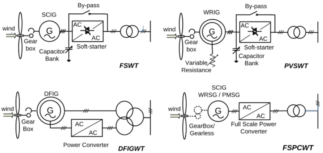
Variable speed WTs are equipped with an induction or synchronous generator connected to the grid through a power converter. The variable speed operation, made possible by means of power electronics, allows such WTs to work at the maximum conversion efficiency over a wide range of wind speeds. The most commonly used WT designs can be categorized into four categories [2][3][1][4]:

• fixed speed WTs (FSWT);

• partial variable speed WTs with variable rotor resistance (PVSWT);

• variable speed WTs with partial-scale frequency converter, known as doubly-fed induction

generator-based concept (DFIGWT);

• variable speed WTs with full-scale power converter (FSPCWT).

Fig.1.1 shows the structure of the above concepts. They differ in the generating system (electrical generator) and the way used to limit the captured aerodynamic power above the rated value.

Fixed speed WTs are characterized by a squirrel cage induction generator (SCIG) directly

connected to the grid by means of a transformer [2]. The rotor speedωmechcan be considered locked

to the line frequency fs as very low slip is encountered in normal operation (typically around 2%).

The reactive power absorbed by the generator is locally compensated by means of a capacitor bank following the production variation (5-25 steps)[2]. A soft-starter can be used to provide a smooth 3

(12)

1.2. CONTROL OBJECTIVES Capacitor Bank By-pass AC AC G Gear box wind SCIG Soft-starter FSWT G Capacitor Bank By-pass AC AC Gear box wind WRIG Soft-starter Variable Resistance Gear Box wind DFIG AC AC G Power Converter DFIGWT GearBox/ Gearless wind SCIG WRSG / PMSG AC AC G

Full Scale Power Converter

FSPCWT

PVSWT

Figure 1.1: Wind turbine concepts.

grid connection. This configuration is very reliable because the robust construction of the standard SCIG and the simplicity of the power electronics [2][1].

Partial variable speed WTs with variable rotor resistance use a WRIG connected to the grid by means of a transformer [2][1][5]. The rotor winding of the generator is connected in series with a controlled resistance; it is used to change the torque characteristic and the operating speed in a

narrow range (typically 0−10% above the synchronous speed)[2]. A capacitor bank performs the

reactive power compenastion and smooth grid connection occurs by means of a soft-starter. For a DFIGWT, the stator is directly coupled to the grid while a partial scale power converter controls the rotor frequency and, thus, the rotor speed [2][1][5][6]. The partial scale power converter

is rated at 20%−30% of the WRIG rating so that the speed can be varied within ± 30% of

the synchronous speed. The partial scale frequency converter makes such WTs attractive from the economical point of view. However, slip rings reduce the reliability and increase the maintenance.

Variable speed FSPCWTs are characterized by the generator connected to the grid by means of the full-scale frequency converter [2][1][5]; the converter performs the reactive power compensation and a smooth grid connection [7][8]. Synchronous generators have so far dominated the market for variable speed wind turbines; now induction generators are becoming more popular in WECS industry and also for variable speed applications [7][1].

1.2 Control Objectives

WECSs connected to the grid must be designed to minimize the cost of supplied energy ensuring safe operation, acoustic emission and grid connection requirements. Control objectives involved in WECSs are [1]:

• energy capture;

• mechanical load;

• grid connection requirements.

1.2.1 Energy capture

Variable-speed variable-pitch WTs are usually controlled according to the curve in Fig.1.2; it rep-resents the energy capture capability of a WT in the generated power-wind speed plane.

(13)

CHAPTER 1. INTRODUCTION

As it is shown in Fig.1.2, the range of operational wind speed is delimited by the cut-inVmin and

0 5 10 15 20 25 30 0 500 1000 1500 2000 2500 Wind speed [m/s] Power [W] cut−in speed

(3.5m/s) cut−out speed

(25m/s) rated wind speed

(8m/s)

2

1 3 fixed speed variable pitch operation 4 variable

speed fixed pitch operation

Figure 1.2:Ideal power regulation for a WT.

cut-outVmaxwind speeds. The WT remains stopped beyond these limits. BelowVmin the available

energy is too low to compensate the operational cost whereas above Vmax speed the WT is shut

down to prevent mechanical overload. The selection of theVmax is a trade-off between the following

items [1]:

• constructing the WT robust enough to support high mechanical stress would be economically

unconvenient;

• even though strong winds have large energy content, they occur seldomly so their contribution

to the annual production is negligible.

A good compromise is oftenVmax= 25m/s. The rated mean wind speedVn is the speed at which

the electrical generator works at its rated power. Within the interval [Vmin;Vn], the available power

is lower than the rated value and so the WT is controlled to maximize the captured energy; in this case the WT will typicaly vary the speed proportionally to the wind speed and keep the pitch

angle θfixed (variable-speed fixed-pitch operation). In this operational region, the captured power

is proportional to V3, where V is the mean wind speed. In countries where the wind energy is

dispatched as traditional energy, the captured power has to react based on the set-point given by the dispatched center; it follows that the captured power could be controlled to be less than the available one [2].

AboveVn, the generator is controlled such that the captured power is limited to the rated value

to prevent mechanical overload (fixed-speed variable-pitch operation). In this region the available power in the wind exceeds the rated power, therefore the WT must be operated with aerodynamic efficiency lower than in the previous region.

1.2.2 Mechanical loads

Mechanical loads can cause fatigue damage and thereby reduced lifetime of the WT. Since the overall cost is spread over a shorter period of time, the cost of energy will rise. Mechanical loads can be divided into static loads, which result from the interaction of the WT with the mean wind speed, and dynamic loads, which comprise variation of the aerodynamic torque that propagates down the drive-train and the mechanical structure. The control system of a WT has a very strong impact especially on the dynamic mechanical loads. The control of the electric generator affects the propagation of drive-train loads whereas the pitch control affects the structural loads [1].

(14)

1.3. PROJECT DESCRIPTION

1.2.3 Grid connection requirements

The injection of large amount of wind power into a network might affect the steady state voltage especially in presence of weak grid [9]. To ensure electrical system stability, system operators in many European countries are setting grid connection requirements for wind generators also known as grid codes (GCs). For MW-size WECSs, very high technical demands are required, such as [2][10][7]:

• regulation of active and reactive power;

• frequency and voltage control;

• fast responses under dynamic situation;

• power quality;

• low voltage ride-through capability.

WECSs must provide the power quality required to ensure the stability and reliability of the power system they are connected to and to satisfy the customers connected at the same grid. Voltage and frequency at the point of common coupling (PCC) must be kept as stable as possible [11]. In general, frequency is a quite stable variable. Frequency variations are always due to power unbalance between generation and consumption (e.g. generators accelerate when the supplied power exceeds the consumption, hence increasing the frequency; analogously they slow down when they can not cover the power demands, thereby frequecy decreases). However this is not the case when the WT is connected to an isolated power system or when multi-MW wind farms are connected to the power system [1]. Voltage variations take place as a consequence of variation of the mean wind speed; the amplitude of these variations depend on the impedance of the grid connected at the PCC, on active and reactive power flows. A way of attenuating voltage variations, without affecting power extraction, is to control the reactive power flow. In the past, when fixed speed wind turbine were the State-of-the-Art, the reactive power compensation was performed by means of capacitor bank following the production variation (5-25 steps). Nowadays the most effective way of reactive power control is based on power electronics.

In the next years, the major research challange is directed towards the grid integration of large wind farms to the electrical power grid. It implies that the survival of different WT concepts is strongly connected by their ability to support the grid, to handle faults on the grid and to comply to grid requirements of the utility companies.

1.3 Project description

This project deals with the control of a variable-speed variable-pitch FSPCWT. According to [2], it is the second most common WT concept in the MW range on the market while the most common is the concept based on the DFIGWT. However, the concept FSPCWT has the chance in the next future to become the best solution as the higher cost is balanced by the power quality, harmonic compensation and full grid support by 100% reactive current injection during grid events [2][7].

The real system is represented in Fig.1.3 Tshaf t and ωgen are respectively the torque and the

rotational speed at the generator shaft (high speed shaft). The SCIG is connected to the ac grid through a frequency converter, the so called back-to-back PWM-VSI; it is a bi-directional power converter consisting of two conventional PWM-VSCs (generator and grid side converters). The pitched-controlled WT and the gearbox are not available; therefore they are implemented by means 6

(15)

AC DC Transformer grid Generator side converter SCIG gen shaft T ,ω GearBox wind gear K Generator side converter contol Pitch contol Grid side converter DC AC Grid side converter contol DC link

Figure 1.3: Layout of the real system.

of a torque-controlled permanent magnet synchronous motor (PMSM). The grid-side converter is not used as it would require its own control system; since its control is not included in this project, the grid side converter is substituted by a dc power supply directly connected at the dc link. The power produced by the WT and flowing through the generator side converter, is dissipated by a braking resistor whose current is controlled by the regenerative braking function provided by the converter. According to the above considerations, the layout of the system is modified as presented

in Fig.1.4. The reference torqueTref is produced according to the models of the WT and the wind.

AC DC Generator side converter SCIG gen shaft T ,ω AC AC Frequency Converter AC grid WT + gear box ref T PMSM dc power supply Braking Resistor Generator side converter contol

Figure 1.4:Modified layout of the system.

1.4 Project goals

In this project the control of a variable-speed variable-pitch WT is designed, simulated and imple-mented. Project goals are summarized below:

• overview of wind turbine technology;

• control of the WT in variable speed operation;

• control of the WT in power limitation mode;

• implementation of the overall control system in a dSPACE platform;

• experimental evaluation and validation.

The control of the WT in variable speed operation is performed using the Direct Field Oriented Control (DFOC) [12][13][14]. The control system has been designed and simulated using Mat-lab/Simulink. The variable speed operation requires a maximum power point tracker (MPPT) which

(16)

provides the reference speed to the generator control such that the maximum power is captured by the WT. The ”perturb and observe” algorithm has been used for the tracking; the maximum power point (MPP) tracker system has been designed and simulated. The control in power limitation mode is performed when the mean wind speed is above the rated value to avoid mechanical stress on the WT structure [2]. It is based on the control of the pitch angle of blades. The control system has been designed and simulated. The entire control system is finally implemented in a dSPACE system and validated by measurements on the experimental test setup.

(17)

Part II:

Modeling

Part II: Modeling 9

2 Modeling 10

2.1 Wind model . . . 10

2.2 Wind turbine model . . . 12

2.3 Drive train model . . . 14

2.4 Induction machine model . . . 16

2.5 Back-to-back converter . . . 18

(18)

Chapter 2

Modeling

This project is focused on the control of small WT. However such a wind turbine is not a part of the experimental setup and so it must be modelled. The power and torque production of the simulated WT depend on the mean wind speed; however the wind turbulence affects the control of the generator. In order to evaluate the power production and the effect of wind variations on the generator control, a model of the wind must be used.

WTs are normally connected to the electric generator by means of a gearbox (optional) and a drive train [2]. They are not a part of the experimental setup and so they must be modelled. The drive train model must take into account the stiffness and damping of the shaft since they will affect the speed at the high speed shaft (generator side).

The control of the SCIG in variable speed mode and in power limitation mode has been designed and simulated in the follwing chapters. Simulation models require a model of the full scale power converter which is a back-to-back frequency converter and a model of modulation method. The models are presented in this chapter.

In variable speed operation, such as at mean wind speeds below the rated value, the WT is operated in order to maximize the enegy capture. This requires a control system that provides the generator

reference speed ω_r∗ to the generator control system. This control system is called Maximum Power

Point Tracker and it is presented in this chapter.

2.1 Wind model

Reliability, performance and cost evaluation of WECSs requires simulation of long-term wind speed data. Winds are movements of air masses in the atmosphere mainly originated by temperature differences. Wind is characterized by its speed and direction, which are affected by several factors.

In the lower layer of the atmosphere, up to 100m, winds are delayed by frictional forces and obstacles

altering not only their speed but also their direction; this is the origin of turbulence flow, which causes wind speed variations over a wide range of amplitudes and frequencies [15]. An interesting characterization of winds in the lower layer is the kinetic energy distribution in the frequency domain, which is known as Van der Hoven spectrum (see Fig.2.1) [1]. Although there are some differences, the kinetic energy distribution in the frequency domain in different sites follow the

same pattern. It exhibits two peaks approximately at 4−days cycles and 1 min. cycles which

are separeted by an energy gap. The concentration of kinetic energy around two clearly separeted

frequencies allows splitting the wind speedvinto two components, the mean wind speedV and the

turbulencevT [1]

v=V +vT (2.1)

(19)

CHAPTER 2. MODELING

Figure 2.1:Van der Hoven spectrum

Usually, the averaging period is chosen to lie within the energy gap, typically 10 min. to 20min.

minutes V = 1 tp Z to+tp₂ to−tp₂ v(t)dt (2.2)

The knowledge of the mean wind speed expected at a specific site is crucial to determine the economical feasibility of a wind energy project. Its value can be determined from measurements

collected during several years. The termvT denotes the atmospheric turbulence which includes all

wind speed fluctuations with frequencies above the spectral gap; therfore it contains all compo-nents in the range from seconds to minutes. Turbulence has a minor impact on the annual energy capture, which is mainly determined by the mean wind speed. However it has a major impact on the aerodynamic loads and power quality [1].

In the wind model, the wind turbulence at a given point in space is stochastically described by means of its power spectrum based on the Kaimal model [1][15]:

Φ(ω) = KV (1 +ωTV) 5 3 (2.3) where KV = 9.316σv2 Lv V (2.4) TV = 2.2240 Lv V (2.5)

The Kaimal model is characterized by the longitudinal lenght scaleLv and the turbulence intensity

σv, which is also the wind speed standard deviation; bothLv andσv are specific to the terrain and

are experimentally obtained from wind speed measurements. The lenght scale takes values ranging

from 100m to 330m whereas the turbulence intensity takes vales between 0.1 and 0.2 [1]. In order

to fit results obtained by means of the Kaimal model with experimenal results, shaping filters are used.

Real wind affects wind turbines in ways that the spectral method does not take into account. Three major effects should be consided when modeling wind turbines [16][1]:

• rotational sampling, which is the fluctuation of the wind experienced by a rotating point;

(20)

2.2. WIND TURBINE MODEL

• wind shear, which is the delay of the wind in the lower layer of the atmosphere due to friction

forces produced by the ground even in absence of obstacles;

• tower shadow, which is the effect on the airflow produced by the tower (3P effect).

Those effects contribute to the turbulence in a deterministic way. The wind model takes into account tower shadow and rotational sampling. Required parameters for the wind model are:

• rotor diameter D;

• average wind speed V;

• length scaleLv;

• turbulence intensity σv;

• sample time Ts.

The wind acting on the considered wind turbine (blade radius R = 2.235 m) has been simulated

using the following parameters:

• V = 8 m/s;

• σv = 12%;

• Lv = 200 m;

• Ts= 0.05 s.

Figure 2.2: Wind time series.

2.2 Wind turbine model

The WT converts the wind energy to mechnical energy by means of a torque applied to a drive train. A model of the WT is necessary to evaluate the torque and power production for a given wind speed and the effect of wind speed variations on the produced torque.

The torque TW T and power PW T produced by the WT within the interval [Vmin, Vmax] are

proportional to the WTs blade radius R, air pressure ρ, wind speed v and a coefficients CQ and

CP [1] [6]. TW T = 1 2ρπR 3_C Q(λ, θ)v2 (2.6) PW T = CP(λ, θ)PV = 1 2ρR 2_C P(λ, θ)v3 (2.7) 12

(21)

CHAPTER 2. MODELING

CP is known as the power coefficient and characterizes the ability of the WT to extract energy

from the wind. CQ is the torque coefficient and is related toCP according to:

CQ =

CP

λ (2.8)

Here, λis the tip-speed-ratio,

λ=ωW TR/v (2.9)

where ωW T is the WT rotor speed.

As seen from (2.6), (2.7) and (2.8) theTW T andPW T depend both on the coefficientCP; which

is normally provided by the manufacturer in the form of a lookup table. However, since there is no

data available for a 2.2 kW WT an equation describing CP is required to calculate TW T andPW T.

An alternative way to calculateCP is based on an approximation from [6] shown in (2.10).

CP(λ, θ) = 0.22 ₁₁₆ λi −0.4θ−5 e −12.5 λi _(2.10)

where θis the pitch angle and λi is described by the equation:

1 λi = 1 λ+ 0.08θ − 0.035 θ3_{+ 1} (2.11)

As seen from (2.10),CP varies with the tip-speed ratioλwhich is dependent on R. In order to

create a the CP curve R has to be defined. Since there is no physical WT in the project, R can

be selected. It is convenient that the generator produces the rated power for the most probable

wind speed of the location; it is assumed to beVn= 8m/s. This gives a requirement for the size of

the WT blades which is consequently calculated to be R= 2.235m; using this value, the generator

should produce the rated power of 2.2kW atVn.

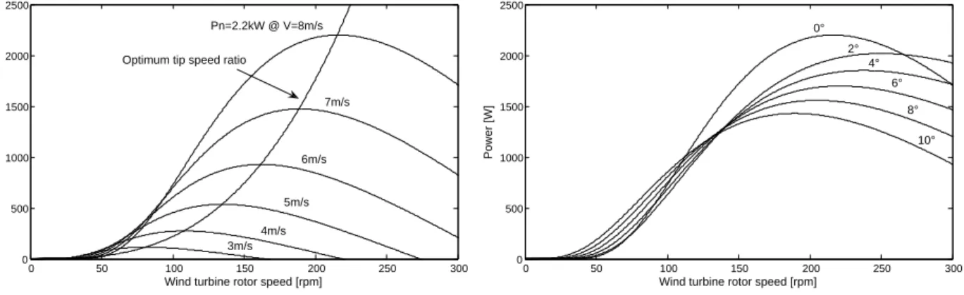
Graphs for the WT power and torque are created using the approximated CP from (2.10).

Fig.2.3 shows how PW T varies with rotor speed for different wind speeds. The optimum tip speed

ratio curve gives the highest efficiency points forPW T. As seen from the figure; the maximum power

is 2.2kW atVn. Fig.2.4 shows how PW T varies with ωW T for different θ at the rated mean wind

speedVn. MaximumPW T is reached forθ= 0◦ but asθis increased, PW T decreases. This is useful

to prevent mechanical overloading of the WT when wind speed exceedsVn.

0 50 100 150 200 250 300 0 500 1000 1500 2000 2500

Wind turbine rotor speed [rpm]

Power [W] Pn=2.2kW @ V=8m/s 7m/s 6m/s 5m/s 4m/s 3m/s Optimum tip speed ratio

0 50 100 150 200 250 300 0 500 1000 1500 2000 2500

Power [W] 0° 2° 4° 6° 8° 10°

Figure 2.3: Power as a function of rotor speed

for different wind speeds.

Figure 2.4: Power as a function of rotor speed for

different pitch angles atVn.

(22)

2.3. DRIVE TRAIN MODEL

Fig.s 2.5 and 2.6 show similar curves as the above mentioned figures but the WT torque TW T

is examined. As for PW T,TW T varies similarly withωW T and θ.

0 50 100 150 200 250 300 0 20 40 60 80 100 120

Torque [Nm]

Tn=111.3Nm @ V=8m/s

Optimum tip speed ratio

7m/s 6m/s 5m/s 4m/s 3m/s 0 50 100 150 200 250 300 0 20 40 60 80 100 120

Torque [Nm] 0° 2° 4° 6° 8° 10°

Figure 2.5: Torque as a function of rotor speed. Figure 2.6: Torque as a function of rotor speed for

different pitch angles atVn.

v R WT ω WT ω v λ 1 035 . 0 08 . 0 1 3₊ − + θ θ λ i λ 1 θ i e i λ θ λ 5 . 12 5 4 . 0 116 22 . 0 − ⎟⎟ ⎠ ⎞ ⎜⎜ ⎝ ⎛ − − CP λP C CQ 2 3 2 1 v C R Q ρπ a WT T , WT T

[

]

0 1 ; , max min Else V V v If = AVG 5 sec

Figure 2.7: Block diagram of WT model.

The block diagram of the WT model for the WT is shown in Fig.2.7. The model has the following inputs:

• WT speedωW T, obtained from a speed meter;

• wind speed v, obtained from the wind model;

• pitch angleθ, obtained from the pitch controller.

As seen from the block diagram the WT model takes the operational wind speed range of the

WT into account; if v, averaged over 5s, hits outside [Vmin; Vmax], the available torque TW T,a is

forced to be zero. The resulting torque TW T is the torque produce by the WT.

2.3 Drive train model

A model of the drive train is required as it has influence on grid interconnectionon by producing power fluctuations. Other mechanical dynamics, such as tower and flap bending modes, are negli-gible from this point of view [17][18]. A two mass model on the generator side has been used; it is 14

(23)

CHAPTER 2. MODELING

represented in Fig.2.8 whereJ_{W T}0 and Jgen are respectively the moment of inertia of the wind

tur-' e K ' e

D

gen

J

' WT

J

' WT

T

' WT

ω

shaft

T

g

ω

Figure 2.8: Equivalent two-mass model of the wind turbine frive train on the generator side

bine, referred to the generator side, and of the generator. The moment of inertia for the low speed shaft, high speed shaft and the gear box wheels can be neglected because they are small compared

with J_{W T}0 and Jgen. Therefore the resultant model is essentially a two-mass model connected by a

flexible shaft characterized by the equivalent torsional stiffness K_e0 and the damping factorD0_e.

The drive train converts the aerodynamic torque produced by the WT,TW T, into a torque at

the high speed shaftTshaf t. This conversion is mathematically described by the following differential

equations [18][17]: ωk =ωg−ω 0 W TKgear (2.12) ˙ θk=ωk (2.13) ˙ ω_{W T}0 = T 0 W T −Tshaf t J_{W T}0 (2.14) Tshaf t=D 0 e(ωg−ωW TKgear) +K 0 eθk (2.15)

where T_{W T}0 is the WT torque referred at the high speed shaft, ω_{W T}0 is the WT rotor speed,Tshaf t

is the torque applied at the rotor of the generator and ωg is the generator mechanical speed.

Parameters used for modeling the drive train are presented in Tab.2.1. The drive train model,

J_{W T}0 0.5 kgm2 K_e0 30 N m/rad D_e0 1 N ms/rad Kgear 7.4 ωg(0) 78.87 rad/s ω_{W T}0 (0) 78.8/7.4 rad/s

Table 2.1:Parameters of the drive train.

whose parameters are listed in Tab.2.1, has been simulated with:

• constant generator speed ωgen =ωgen,n;

• step variation of the WT torque from T_{W T}0 =T_{W T,n}0 /2 toT_{W T}0 =T_{W T,n}0 att= 2 s.

Simulation results are shown in Fig.s 2.9 and 2.10.

(24)

2.4. INDUCTION MACHINE MODEL 0 0.5 1 1.5 2 2.5 3 3.5 4 0.1 0.11 0.12 0.13 0.14 0.15 0.16 0.17 Time [s] Speed [p.u.] w_g/K_gear w_WT

Figure 2.9: Speed response of the drive train.

0 0.5 1 1.5 2 2.5 3 3.5 4 0 5 10 15 20 Time [s] [Nm] T_shaft T_WT/K_gear

Figure 2.10: Torque response of the drive train.

Fig.s 2.9 and 2.10 show that torque and speed oscillations are introduced by the drive train. If

it was infinitely stiff, then it would be ω0_{W T} =ωg and Tshaf t=T

0

W T. This makes the control of the

generator more difficult as Tshaf t is a disturbance.

2.4 Induction machine model

In this section the model of the induction machine in the rotating dq reference frame is derived.

First, equations in the αβ stationary reference frame are obtained. The α-axis is aligned with the

stator a-axis, as shown in Fig.2.11. In such reference frame the induction machine can be represented

Figure 2.11: Statorαβ and dq equivalent windings.

(25)

CHAPTER 2. MODELING

by means of space vectors as follows [19][20][21][13]: ¯

vsαβ =Rs¯isαβ+

d¯λsαβ

dt (2.16)

The current ¯isαβ, voltage ¯vsαβ and stator flux linkage ¯λsαβ space vectors with respect to theα-axis

are represented in the rotating dq reference frame as follows (see Fig.2.11): ¯

vsαβ = ¯vsdq·ejθdq (2.17)

¯_i_sαβ _{= ¯}_i_sdq_·_ejθdq _(2.18)

¯

λsαβ = ¯λsdq·ejθdq (2.19)

whereθdq is he angle between the statorα-axis and the d-axis. Substituting (2.17), (2.18) and (2.19)

into (2.16) ¯ vsdq·ejθdq =Rs¯isdq·ejθdq+ d dt¯λsdq·e jθdq _(2.20) Hence ¯ vsdq=Rs¯isdq+ dλ¯sdq dt +jωdq ¯ λsdq (2.21)

Using a similar approach, the rotor voltage equations in the δγ reference frame, rotating atωr, can

be obtained [13].

¯

vrδγ = 0 =Rs¯irδγ+

dλ¯rδγ

dt (2.22)

Since the rotor is short circuited, ¯vrδγ = 0. In order to obtain a model of the induction machine,

both stator and rotor variables must be represented in the same reference frame. Beingθrthe angle

between the rotor δ-axis and the statorα-axis, it yields

¯

λrδγ = ¯λsαβ·e−jθr (2.23)

¯_i_rδγ _{= ¯}_i_sαβ·e−jθr _(2.24)

Substituting (2.23) and (2.24) in (2.22) and multiplying by ejθr _{the rotor voltage equation in the}

αβ reference frame is obtained

¯ vrαβ = 0 =Rr¯irαβ + dλ¯rαβ dt −jωr ¯ λrαβ (2.25)

The current, voltage and flux linkage rotor space vectors with respect to the α-axis are represented

in represented in the rotating dq reference frame as follows ¯

vrαβ = ¯vrdq·ejθdq (2.26)

¯_i_rαβ _{= ¯}_i_rdq_·_ejθdq _(2.27)

¯

λrαβ = ¯λrdq·ejθdq (2.28)

whereθdq is he angle between the statorα-axis and the d-axis. Substituting (2.26), (2.27) and (2.28)

into (2.25) ¯ vrdq·ejθdq =Rr¯irdqejθdq + d dt ¯ λrdqejθdq −jωr¯λrdqejθdq (2.29) Hence ¯ vrdq = 0 =Rr¯irdq+ d dtλ¯rdq −j(ωr−ωdq)¯λrdq (2.30) 17

(26)

2.5. BACK-TO-BACK CONVERTER

(2.21) and (2.30) can be written as function of the stator current space vector ¯isdq and the rotor

linkage flux space vector λ0_rdq. After mathematical manipulation [13]

¯ vsdq =Rs¯isdq+σLs d¯isdq dt +jωdqσLs¯isdq+ LM L0_r d dt ¯ λ0_rdq+jωdq LM L0_r ¯ λ0_rdq (2.31) 0 =−σrLM¯isdq+σrλ¯ 0 rdq+ d dtλ¯ 0 rdq+j(ωdq −ωr)¯λ 0 rdq (2.32) where ¯ λ0_rdq =L0_r¯i0_rdq+LM¯isdq (2.33)

is the rotor flux linkage referred to the stator side

σ= 1− L

2

M

L0_rLs

(2.34) is the dispersion factor and

σr= R0_r L0_r = 1 TR (2.35)

is the inverse of the rotor time constantTR.

2.5 Back-to-back converter

A back-to-back converter consists of two voltage source converters (VSC) and a capacitor as shown in Fig.2.12. When operating in generator mode, the generator side converter operates as a rectifier and the grid side converter as an inverter. But as both converters are identical, power flow can be bi-directional [17][22].

DC

Figure 2.12: Back-to-back converter.

Model of the back-to-back converter is necessary in simulation to feed the generator model. But as the generator side is only considered in simulations, the model of the whole back-to-back converter is not needed. Consequently, the model of the generator side VSC is sufficient to carry out the simulations and is the only part considered in this section. The model of the VSC is an average model as the system includes a mechanical system making the time-frame of interest much longer than the switching time of the converter. Therefore, there is no need to have a switching model where the effect of switching adds little significance to the result.

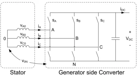
For a star connected generator, the generator side voltagesvA0,vB0 andvC0, shown in Fig.2.13,

can be calculated using (2.36)-(2.38) where vAN, vBN and vCN are the line-to-neutral voltages,

(27)

CHAPTER 2. MODELING A0 B0 C0 A B C A B C DC 0N DC

Figure 2.13:Star connected generator and generator side VSC.

between the specified points A, B or C and the neutral point N. As the average model is used,

vAN,vBN andvCN are average voltages andsA,sB and sC are duty cycles.

vA0 = vAN−v0N =sAVDC−v0N = VDC 3 (2sA−sB−sC) (2.36) vB0 = vBN −v0N =sBVDC−v0N = VDC 3 (−sA+ 2sB−sC) (2.37) vC0 = vCN −v0N =sCVDC−v0N = VDC 3 (−sA−sB+ 2sC) (2.38) where v0N is defined as [23]: v0N = 1 3(vAN+vBN +vCN) = VDC 3 (sA+sB+sC) (2.39)

The dc link currentiDC can be expressed as:

iDC = h sA sB sC i    iA iB iC    (2.40)

The model of the VSC is shown in Fig.2.14 whereGainis explained in (2.41), it is the matrix

notation of (2.36)-(2.38).    vA0 vB0 vC0   =VDC    2 3 − 1 3 − 1 3 −1 3 2 3 − 1 3 −1₃ −1₃ 2₃    | {z } Gain    sA sB sC    (2.41) 2.5.1 Modulation

The VSC requires duty cyclessA,sBandsCin order to control the power flow through the converter.

Space vector modulation (SVM) is chosen because it has higher utilization of the dc voltage than 19

(28)

2.5. BACK-TO-BACK CONVERTER ⎥ ⎥ ⎥ ⎦ ⎤ ⎢ ⎢ ⎢ ⎣ ⎡ C B A i i i

[

sA sB sC

]

Dot product Product X Gain DC V

[

vA0 vB0 vC0

]

DC i

Figure 2.14: Model of the VSC.

the sinusoidal PWM method and does not require seperate modulators and calculation of

zero-sequence signals as in third harmoninc PWM [24]. SVM uses the stationary αβ reference frame

where the reference voltage space vector Vref is defined as follows:

Vref =

2 3

vAref +αvBref+α2vCref

(2.42) where α=−1 2+j √ 3

2 and vAref,vBref and vCref are the reference voltages.

The defintion of Vref depends on its location within the reference frame. In Fig.2.15, Vref is

located in sector 1 and is therefore defined by the state voltages V100and V110.V110 is the voltage

produced by the state [1 1 0] where the upper switches in the first and middle leg of the VSC are

conducting. Tpwm is the switching period of the VSC and γ is the phase angle of Vref.

V100= vα V110 V010 V011 V001 V101 2t1 2t2 Tpwm Tpwm V100 V110 Vref

1

2

3

4

5

6

vβ V111 V000 γ

Figure 2.15: Vref located in sector 1.

As shown in Fig.2.16, the switching of states occurs in the following order [0 0 0], [1 0 0], [1 1 0], [1 1 1] to reduce the number of switching commutations [25][26][27]. The states [0 0 0] and [1 1 1] are referred to as zero states as no power flows through the VSC during their activity. Other 20

(29)

CHAPTER 2. MODELING

states are referred to as active states. In SVM the zero states are symmetrical, that is [24]:

t7 =t8= Tpwm 2 −t1−t2= t0 2 (2.43) t0 t1 t2 t7 000 100 110 111 Tpwm 2 1 _T pwm 2 1

Figure 2.16:The state sequence.

Vref in sector 1 can then be expressed as:

Vref =V100 t1 Tpwm 2 +V110 t2 Tpwm 2 (2.44)

where the state voltages are:

V100 = 2 3 α0VDC·1 +α1VDC·0 +α2VDC·0 = 2 3VDC (2.45) V110 = 2 3 α0VDC·1 +α1VDC·1 +α2VDC·0 = 2 3VDC 1 2 +j √ 3 2 ! (2.46)

The time durations,t1 andt2, can be calculated using (2.44) by splitting to real and imaginary

part, where Vref =Vref(cosγ+jsinγ):

RehVref i = Vrefcosγ = 2 3VDC t1 Tpwm 2 +2 3VDC t2 Tpwm 2 cos 60◦ (2.47) ImhVref i = Vrefsinγ= 2 3VDC t2 Tpwm 2 sin 60◦ (2.48)

The time durations for the states [1 0 0] and [1 1 0], are then [24]:

t1 = √ 3Vref VDC Tpwm 2 sin (60 ◦₋_γ₎ _(2.49) t2 = √ 3Vref VDC Tpwm 2 sinγ (2.50)

Finally, the duty cycles of the output phase voltages vA0, vB0 and vC0 can be calculated for

sector 1: sA = t1+t2+T₂0 Tpwm 2 (2.51) 21

(30)

sB = t2+T₂0 Tpwm 2 (2.52) sC = T0 2 Tpwm 2 (2.53)

The duty cycles can be obtained for other sectors in similiar fashion. Expression for time dura-tions, valid for all sectors, can be found in [28].

(31)

Part III:

Control System Design

Part III: Control System Design 23

3 Maximum power point tracking 25

3.1 Output filter design . . . 27

3.2 Selecting step size . . . 29

4 Control of the generator in variable speed operation 31

4.1 Introduction . . . 31

4.2 Rotor flux vector estimation . . . 32

4.2.1 Current model . . . 32

4.2.2 Voltage model . . . 33

4.3 Field Oriented Control . . . 35

4.3.1 Electromagnetic torque in the dq reference frame . . . 36

4.4 Control system design . . . 38

4.4.1 Q-axis control loop design . . . 38

4.4.2 D-axis control loop design . . . 47

4.5 Simulation on the generator control in variable speed operation . . . 55

4.5.1 Case 1: variable wind speed and constant reference rotor speed . . . 55

4.5.2 Case 2: variable wind speed and variable reference rotor speed (with MPPT) 57

4.5.3 Case 3: variable rotor reference speed and constant mean wind speed . . . 60

4.5.4 Case 4: variable reference rotor speed and variable mean wind speed . . . 62

5 Power limitation mode 65

5.1 Pitch control . . . 65

5.2 Assessment of pitch controller model . . . 66

5.3 Transition between variable speed operation and power limitation mode . . . 68

5.4 Simulation in variable pitch operation . . . 68

5.4.1 Case 1: variable wind in power limitation mode . . . 69

5.4.2 Case 2: reference power profile in power limitation mode . . . 69

(32)

(33)

CHAPTER 3. MAXIMUM POWER POINT TRACKING

Chapter 3

Maximum power point tracking

As seen in Fig.2.3 the output power of the WT varies with the rotor speed. While working in the variable speed region, the WTs efficiency can be considerably increased by varying the rotor speed to the maximum power point.

The MPPT could be implemented by calculating the reference WT speed ω∗_{W T} using the

opti-mum tip-speed ratioλopt and (3.1) as described in [29][30][31].

ω_{W T}∗ = vλopt

R (3.1)

Block diagram of (3.1) is shown in Fig.3.1 whereKgearis the gear ratio andnp the number of poles.

R opt λ gear

K

n

_p

ω

_r* * mech

ω

* WT

ω

v

Figure 3.1: Block diagram of (3.1).

This should set the system quickly to its MPP, given thatλopt is in fact the optimum value. But

because λopt changes during the systems lifetime, it needs to be maintained at the optimum value

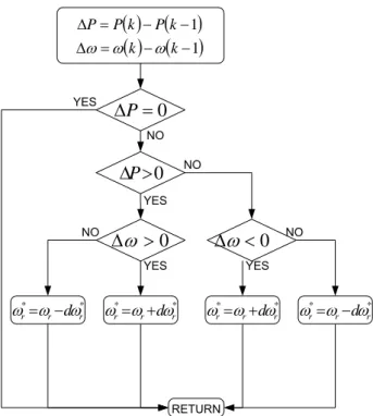
by the use of an adaptive system [30]. This is difficult to implement and it is therefore considered a better approach to implement the MPPT using the simple ”perturb and observe” method. This method is slower than the previously mentioned method but it does not require any parameters. The measured power and speed of the generator are fed to buffers which hold the values for one period. They are then compared to their values of next sampling period. Depending if they have

increased or decreased, the generator reference speedω_r∗is increased or decreased by a constant step

size dω_r∗. The ”pertub and observe” method used is based on [32] and [33] for PV panels. Similar

method is described in [34] for WTs but it lacks the tracking of MPPT when ωW T has exceeded

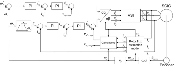
the MPP speed and needs to be reduced. The flowchart of the MPPT method is shown in Fig.3.2. The MPPT has been implemented with an S-function builder in Simulink. Fig.3.3 shows the structure of the whole system including the MPPT controller. Inputs to the MPPT controller are

measured power Pg which can be either the generator power or the WT mechanical power, the

measured generator electrical rotor speed ωr and a user-defined step sizedω∗r.

(34)

( ) (

− −1

)

= ΔP Pk Pk 0 > ΔP 0 < Δ

ω

0 > Δ

ω

( ) (

− −1

)

= Δω ωk ωk 0 = ΔP * * r r r ω dω ω = − * * r r r ω dω ω = + * * r r r ω dω ω = + * * r r r ω dω ω = −

Figure 3.2: Flowchart of MPPT method.

s

v

MEAN WIND SPEED PROFILE

WIND MODEL WT MODEL DRIVE TRAIN

MODEL SCIG Control MPPT VCI DC BUS − duty cycles V

v

CHAPTER 3. MAXIMUM POWER POINT TRACKING

3.1 Output filter design

To minimize oscillations of the generator electrical rotor speedωr, a filter is applied. The selection

of filter is made by inspection of 1st order filters with different time constants τ:

H(s) = 1

τ s+ 1, τ =

h

90−1,100−1,200−1,400−1i (3.2)

Time constants for testing are chosen arbitrarily but it should be noted that the MPPT controller

does not track for values higher than τ = 90−1 s. The system used in the simulation is shown in

Fig.3.4 and is simulated with a fixed step of 1/Fs = 0.2 ms, where Fs = 5kHz. Delays are set to

hold its inputs for one time step.

+ -g P Delay r ω * r ω Filter Delay θ V r ω Wind Speed Pitch + -Delay Step size * r dω Perturb and Observe S-function r ω Power Calculation

Figure 3.4: Block diagram of simulation model.

This model does not take into account:

• the WT inertia (it would limits the rate of change in speed);

• the wind speed turbulence (it would produces power oscillations);

• drive train and gear box (it is assumed ωW YKgear=ωr/np;

• effects of the generator control (the error betweenω∗_r and ωr is neglected);

The last point implies that ω_r∗ and ωr are the same, meaning that the generator aligns

in-stantaneously with the reference speed. This does not reflect the operation of the real system but is considered enough to check the functionality of the MPPT and to examine different output filters. The model uses (2.10) and (2.7) to calculate the power produced by the WT for the measured

electrical speed of the generator ωr. The pitch angle is irrelevant for the simulation and is set to 0.

An additional delay is necessary between the output ω∗_r and the inputωr to avoid algebraic loops

(36)

3.1. OUTPUT FILTER DESIGN

during the simulation. The optimum speed ωopt is calculated using (3.1); it is used to compare the

results.

Fig.3.5 shows the wind profile where the mean wind steps up fromVmin = 3.5m/stoV = 5m/s.

Fig.3.6 shows the response of ω_r∗ for different τ. Fig.s 3.7 and 3.8 show ω∗_r and the wind profile

where the mean wind speed steps fromVmin= 3.5m/stoVn= 8m/s.

0 0.5 1 1.5 2 2.5 3 3.5 4 4.5 5 3 3.5 4 4.5 5 5.5 Time [s] Wind speed [m/s] 2.4 2.45 2.5 2.55 2.6 2.65 2.7 2.75 2.8 0.65 0.7 0.75 0.8 0.85 0.9 0.95 1 1.05 Time [s] Speed [p.u.] τ = 1/400 s τ = 1/200 s τ = 1/100 s τ = 1/90 s

Figure 3.5: Wind profile. Figure 3.6: Response of ω∗_r for different time

con-stants. 0 0.5 1 1.5 2 2.5 3 3.5 4 4.5 5 3 3.5 4 4.5 5 5.5 6 6.5 7 7.5 8 8.5 Time [s] Wind speed [m/s] 2.4 2.45 2.5 2.55 2.6 2.65 2.7 2.75 2.8 0.4 0.5 0.6 0.7 0.8 0.9 1 1.1 Time [s] Speed [p.u.] τ = 1/400 s τ = 1/200 s τ = 1/100 s τ = 1/90 s

Figure 3.7: Wind profile. Figure 3.8: Response of ω∗r for different time

con-stants.

Simulation results are gathered in Tab.s 3.1 and 3.2 where ωss is the steady state speed, δωss

is the deviation from ωopt, ∆ss is the steady state error and tres is the response time that the

controller needs to reach 90% of ωopt. This is further explained in Fig.3.9.

(37)

CHAPTER 3. MAXIMUM POWER POINT TRACKING τ [s] ωss [p.u.] δωss [%] ∆ss [%] tres [ms] 90−1 1.0000 0.0011 2.28 32.0 100−1 1.0000 -0.0040 2.53 29.0 200−1 1.0001 0.0118 5.00 14.6 400−1 1.0001 0.0207 9.76 7.8

Table 3.1:Simulation results corresponding to Fig.3.6.

τ [s] ωss [p.u.] δωss [%] ∆ss [%] tres [ms]

90−1 1.0000 0.0025 3.55 118.4

100−1 1.0000 -0.0013 2.53 106.8

200−1 0.9999 -0.0072 5.00 54.4

400−1 1.0000 0.0041 9.76 28.4

res opt opt ss ss ss (cut-in)

Figure 3.9: Measured parameters explained.

As Tab.s 3.1 and 3.2 show in most cases, speed ripple increases and reponse time decreases with lower time constant. Since there are no design requirements, it can not be said which time constant should be used; however it has to be considered

• because of high inertia of the WT, the speed cannot change very quickly which puts less

significance to faster response;

• speed ripple produces torque ripple and reduces the voltage quality of the electrical

produc-tion.

According to the above considerations, a slow time constant would produce a small speed ripple

and an acceptable slow response. However τ = 90−1_s_{produces an higher ripple than} _τ _{= 100}−1_s

and therefore the time constant for the filter is chosen to be τ = 100−1 s.

3.2 Selecting step size

The analysis to determine suitable step size dω∗_r for the MPPT is simulated using the same model

as before from Fig.3.4. Four different step sizes are tested:

(38)

3.2. SELECTING STEP SIZE

dω_r∗ = [1,2,5,9]

Wind profiles are the same as in Fig.s 3.5 and 3.7; the sampling time is again 1/Fs = 0.2 ms

and the output filter is the one selected previously withτ = 100−1 s.

Fig.s 3.10 and 3.11 show ω∗_r for different dω_r∗. Simulation results are gathered in Tab.s 3.3 and

3.4. 2.4 2.45 2.5 2.55 2.6 2.65 2.7 2.75 2.8 0.4 0.45 0.5 0.55 0.6 0.65 Time [s] Speed [p.u.] dω* r = 9 rad/s dω* r = 5 rad/s dω* r = 2 rad/s dω* r = 1 rad/s 2.4 2.45 2.5 2.55 2.6 2.65 2.7 2.75 2.8 0.4 0.5 0.6 0.7 0.8 0.9 1 1.1 Time [s] Speed [p.u.] dω* r = 9 rad/s dω* r = 5 rad/s dω* r = 2 rad/s dω* r = 1 rad/s

Figure 3.10:Response for cut-in wind speed with

different step sizes.

Figure 3.11:Response for rated wind speed with

dif-ferent step sizes.

dω∗_r [rad/s] ωss [p.u.] δωss [%] ∆ss [%] tres [ms]

1 1.0000 -0.0040 2.53 29.0

2 1.0000 0.0017 7.88 14.4

5 1.0002 0.0213 19.70 5.8

9 0.9999 -0.0076 22.74 3.2

dω∗_r [rad/s] ωss [p.u.] δωss [%] ∆ss [%] tres [ms]

1 1.0000 -0.0013 2.53 106.8

2 1.0001 0.0122 7.88 53.4

5 1.0000 0.0006 16.47 21.4

9 0.9999 -0.0105 22.74 11.8

As simulation results reveal, ∆ss increases and tres decreases with increasing dωr∗. While the

influence of faster response will probably never be seen because of the intertia of the WT, the speed

ripple and more accurate MPPT are considered to outweight the response time. Thereforedω_r∗= 1

is chosen as step size.

(39)

CHAPTER 4. CONTROL OF THE GENERATOR IN VARIABLE SPEED OPERATION

Chapter 4

Control of the generator in variable

speed operation

4.1 Introduction

A variable-speed variable-pitch WT is controlled as represented in Fig.4.1 such that [1][2]:

• when the mean wind speed V < Vmin (region 1), the WT rotates but is not connected to the

grid because the power production is not enough to cover the operational cost;

• when Vmin ≤V ≤Vn (region 2), the WT is operated at variable-speed mode such that the

captured power is maximized; the pitch angle is kept to the optimum value, ideally zero; • when V < Vm ≤Vmax (region 3), the WT works at variable-pitch operation for limiting the

captured power to the rated one; the WT rotor speed is then kept constant;

• with V > Vmax (region 4), the WT is stopped by means of the pitch control system to avoid

mechanical overloading; in this case mechanical breaks are normally not enough so blades are pitched to very small angle of attack.

0 5 10 15 20 25 30 0 500 1000 1500 2000 2500 Wind speed [m/s]

Power [W] cut−in speed

(3.5m/s) cut−out speed

(25m/s) rated wind speed

(8m/s)

2

1 3 fixed speed variable pitch operation 4

variable speed fixed pitch operation

Figure 4.1:Ideal power regulation for a WT.

Depending on the WT operation region in Fig.4.1, different control strategies are used for perform-ing the desired action.

(40)

4.2. ROTOR FLUX VECTOR ESTIMATION

This chapter is entirely focused on the variable speed operation of the WT (region 2). In this region, the electric generator is controlled to rotate at the speed which corresponds to the maximum

power coefficient CP max. Thus, a speed control system is used. The generator reference speed ωr∗

is obtained by implementing a Maximum Power Point Tracker (MPPT) algorithm which changes the reference generator speed towards the point where the maximum captured power is achieved [34]. The speed control of the electric generator is implemented by controlling the generator side converter.

Induction machines are difficult to control because of their highly non-linear dynamic structure

with strong interactions [35][21]. Due to dynamic interactions between phases, the control in theabc

reference frame is not used. The control is normaly performed using the so called ”Field Oriented Control”; it is based on an algebraic transformation that converts the dynamic structure of the induction machine into a decoupled structure with independent control of the rotor flux and torque [12][20][35][21]. The above transformation is based on the reference frame theory, where balanced three-phase system variables are represented by space vectors [19][14].

4.2 Rotor flux vector estimation

Depending on how the rotor flux position θϕ (or speed ωϕ) is estimated, the same control system

can be used for Direct Field Oriented Control (DFOC) or Indirect Field Oriented Control (IFOC).

In any cases the FOC is based on the independent control ofisqandisd, thus the rotor flux position

is required as the d-axis is assumed aligned with ¯λ0_rdq. Basic features of both DFOC and IFOC are

briefly analyzed [20]:

• the IFOC is based on the compensation of the estimated slip frequencysωr= σr_λL0M

r

as shown in (4.23); therefore a rotor speed measurement is required.

• in the DFOC the rotor flux estimation is based on the measurements on electrical variables.

In both cases the accuracy of the rotor flux estimation depends on the knowledge of generator pa-rameters. The DFOC has a more complex structure than the IFOC where only the slip compesation

is involved. However in the DFOC the rotor flux αand β components are estimated and therefore

they can be used as monitoring parameters for the assessment of performance of the control system;

meaning that the rotor flux space vector ¯λrαβ =λrα+jλrβ can be plotted and monitored in order

to identify significant disturbances in the system [20]. Since the DFOC provides more information, it has been selected for controlling the SCIG.

Two methods for rotor flux estimation are commonly used [36][20]:

• current model;

• voltage model.

4.2.1 Current model

The current estimation model can be either represented in the αβ stationary reference frame or

in the dq rotating reference frame [13]. The one represented in dq is easier because there are not

cross couplings between axes. Considering adqrotating reference frame aligned with the rotor axis,

(4.14) can be written as follows

¯_i_sdq ₌ λ¯ 0

rdq

LM

(1 +sTr) (4.1)

(4.1) is used in the current model. The following steps can be used for the rotor flux estimation: 32

(41)

• transforming the stator current space vector ¯is(a,b,c)into ¯isdqby means of the Clark (abc→αβ)

and Park (αβ→dq) transformations;

• calculating rotor flux componentsλ0_rq and λ0_rd using (4.1);

• calculating rotor flux components λ0_rα and λ0_rβ using the inverse Park (dq→αβ)

transforma-tion;

• calculating the magnitude λ0_r;

• calculating cosωϕ=λ 0 rα/λ 0 r and sinωϕ =λ 0 rβ/λ 0 r; • calculating isϕ= λ 0 r LM;

• calculating the rotor flux frequency ωϕ by means of the slip compensation equation (4.23).

The block diagram of the current model in the dq reference frame is shown in Fig.4.2. The rotor

abc αβ ) , , (abc s

i

_s_α

ϕ ω sin CURRENT MODEL r θ

Figure 4.2: Current model rotor flux estimation block diagram [13].

flux estimation based on the current model requires the measured speed and thus the encoder, but the advantage is that the estimation is well performed down to zero speed [36]. The estimation accuracy is affected by the variation of machine parameters especially at high speed [36]. For this reason this estimation model is not suitable at high speed.

4.2.2 Voltage model

The rotor flux estimation based on the voltage model requires stator voltages and currents [36][20]; the rotor speed is no longer required yielding to an estimation poor of accuracy at low speed [36].

It is based on the αβ voltage equation of the machine

¯

vsαβ =Rs¯isαβ+

d¯λsαβ

dt (4.2)

Given vsα, vsβ, isα and isβ,, the stator flux components can be calculated as follows:

λsα = Z (vsα−Rsisα)dt (4.3) λsβ = Z (vsβ−Rsisβ)dt (4.4) 33

(42)

4.2. ROTOR FLUX VECTOR ESTIMATION

The magnetizing flux linkage components are

λmα =λsα−Llsisα=LM isα+i 0 rα (4.5) λmβ =λsβ−Llsisβ =LM isβ+i 0 rβ (4.6) The rotor flux components are

λ0_rα=LMisα+L 0 ri 0 rα (4.7) λ0_rβ =LMisβ+L 0 ri 0 rβ (4.8)

Eliminating i0_rα and i0_rα from (4.7) and (4.8) by using (4.5) and (4.6), it yields

λ0_rα = L 0 r LM λmα−Llrisα (4.9) λ0_rα= L 0 r LM λmβ −Llrisβ (4.10)

which can also be written as follow by using (4.5) and (4.6)

λ0_rα = L 0 r LM (λsα−σLsisα) (4.11) λ0_rβ = L 0 r LM (λsβ−σLsisβ) (4.12)

Rs Lls

L

lr β s

i

) , , (abc s

i

Figure 4.3:Voltage model rotor flux estimation block diagram [36].

start-up); furthermore the variation of machine parameters significantly reduces the accuracy of the estimation only at low speed. As a consequence, the voltage model is good at high speed [36].

Since the current model flux estimation is better at low speed and the voltage model is better at high speed, the best solution for the rotor flux estimation is the use of a hybrid model. However in this project, the current model has been selected because it can work at every speed even though the accuracy decreases as the rotor speed increases.

(43)

4.3 Field Oriented Control

An effective method of controlling ac drives in based on the Field Oriented Control (FOC) [37]. It consists of controlling stator currents represented by a space vector in a rotating reference frame whose coordinates are d and q [12][35]. To understand the FOC, a model of the indution machine in the rotating dq reference frame is required; it is thus presented in section 2.4. The electrical model is represented by (4.13) and (4.14) [13]. ¯ vsdq =Rs¯isdq+σLs d¯isdq dt +jωdqσLs¯isdq+ LM L0_r d dt ¯ λ0_rdq+jωdq LM L0_r ¯ λ0_rdq (4.13) 0 =−σrLM¯isdq+σrλ¯ 0 rdq+ d dt ¯ λ0_rdq+j(ωdq −ωr)¯λ 0 rdq (4.14) where ¯ λ0_rdq =L0_r¯i0_rdq+LM¯isdq (4.15)

is the rotor flux linkage referred to the stator side

σ= 1− L

2

M

L0_rLs

(4.16) is the dispersion factor and

σr= R0_r L0_r = 1 TR (4.17)

is the inverse of the rotor time constantTR.

In FOC the d-axis is aligned with the d-axis of rotor flux linkage space vector ¯λ0_rdq. With this

assumption the rotor flux in the dq reference frame is a scalar ¯λ0_rdq =λ0_r and ωdq =ωϕ. (4.13) and

(4.14) can be decomposed into d and q components as follows (_dtd is here substituted by the Laplace

operator)

• d component of the rotor voltage (from (4.14)):

0 =−σrLMisd+σrλ

0

r+sλ

0

r (4.18)

• q component of the rotor voltage (from (4.14)):

0 =−σrLMisq+ωϕλ

0

r−ωrλ

0

r (4.19)

• d component of the stator voltage (from (4.13)):

vsd =Rsisd+σLssisd−ωϕσLsisq+

LM

L0_r sλ

0

r (4.20)

• q component of the stator voltage (from (4.13)):

vsq=Rsisq+σLssisq+ωϕσLsisd+ωϕ LM L0_r λ 0 r (4.21) 35

(44)

4.3. FIELD ORIENTED CONTROL

where isϕ = λ

0 r

LM is the component of the stator current that generates the rotor linkage flux λ

0 r. From (4.18) λ0_r= σrLM σr+s isd= LM 1 +TRs isd (4.22)

(4.22) shows that isd is the command variable for the rotor linkage fluxλ

0

r.

From (4.19) the angular speed of the rotor flux linkage λ0_r is obtained

ωϕ =ωr+

σrLM

λ0_r isq (4.23)

(4.23) shows that the rotor flux speed ωϕ is obtained by adding to the electrical rotor speedωr the

slip speed Sωr = σr_λL0M

r

isq. This is the main characteristic of the Indirect Field Oriented Control

(IFOC). Substituting (4.22) into (4.20)

vsd+ωϕσLsisq= 1 +σTSs+ (1−σ)TS s 1 +TRs Rsisd (4.24)

where TS =Ls/Rs is the stator time constant. From (4.24) the transfer function along the d-axis

is obtained isd = 1 Rs 1 +TRs TSTRσs2+ (σTS+TR)s+ 1 (vsd+ωϕσLsisq) (4.25) Substituting (4.23) into (4.21) vsq−ωϕσLs(isd−isϕ)−ωr Ls LM λ0_r= Rs(TS+TR) TR 1 +σ TSTRs TS+TR isq (4.26)

Defining the equivalent time constant

Ta=σ

TSTR

TS+TR

(4.27) and equivalent resistance

Ra=

Rs(TS+TR)

TR

(4.28) (4.26) can be written as follows

vsq−ωϕσLs(isd−isϕ)−ωr

Ls

LM

λ0_r=Ra(1 +Tas)isq (4.29)

Hence the transfer function along the q-axis is obtained

isq = 1 Ra1 +Tas vsq−ωϕσLs isd−isϕ −ωr Ls LM λ0_r (4.30)

4.3.1 Electromagnetic torque in the dq reference frame

Stator and rotor linkage fluxes can be expressed as functions of the stator and rotor currents as follows ¯ λsαβ =Ls¯isαβ+LM¯i 0 rαβ (4.31) ¯ λ0_rαβ =Lr¯i 0 rαβ +LM¯isαβ (4.32) 36

Institute of Energy Technology, 9 th Semester Report. Control of a variable speed variable pitch wind turbine with full scale power converter