Essays on Libor Manipulation

(1)

Essays on Libor Manipulation

A DISSERTATION

SUBMITTED TO THE FACULTY OF THE GRADUATE SCHOOL OF THE UNIVERSITY OF MINNESOTA

BY

Thomas Youle

IN PARTIAL FULFILLMENT OF THE REQUIREMENTS FOR THE DEGREE OF

Doctor of Philosophy

(2)

c

Thomas Youle 2014

ALL RIGHTS RESERVED

(3)

Acknowledgements

This dissertation could not have been written without the fellow and former graduate students and faculty at the University of Minnesota. Amil Petrin, Thomas Holmes, Patrick Bajari, David Skeie, Richard Todd, Connan Snider and Motohiro Yogo are each owed a special thanks. To my friends and family, without whose support I may never have finished the journey, I am eternally grateful.

(4)

List of Tables

1.1 Monte Carlo of Test on Model Simulated Data . . . 25

1.2 Three Month Dollar Libor Summary Statistics . . . 26

1.3 All Bank Bunching at the 4th Lowest Quote (3M Dollar) . . . 27

2.1 Submitted Quotes (3M USD Libor; Week of 12/17/2007) . . . 65

2.2 Comparison of Pre- and Post-Crisis Interquartile Ranges . . . 66

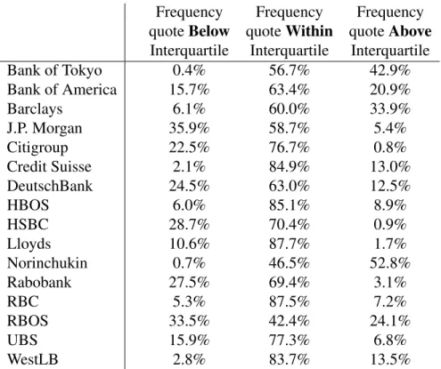
2.3 Summary Statistics by Bank . . . 67

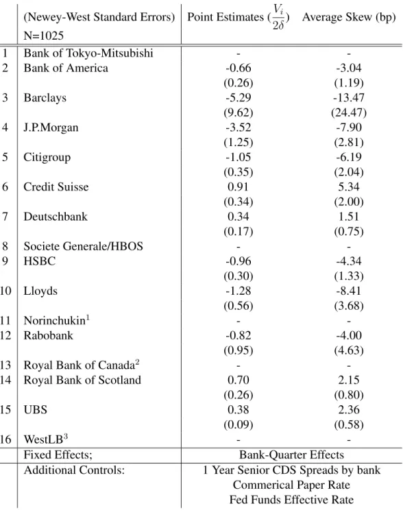
2.4 Estimating Necessary First Order Conditions; Second Stage . . . 68

(7)

List of Figures

1.1 Libor - Eurodollar Bid Rate (1/2005-7/2012) . . . 28

1.2 Costs vs. Quotes in Model of Manipulation . . . 29

1.3 Simulated Distribution of Quotes Minus Daily 4th Lowest of 15 Other Banks . . . 30

1.4 All Banks: 3M Bank Quote Minus the 4th Lowest of Fifteen Other Banks 31 1.5 All Banks: 3M Bank Quote Minus the 4th Highest of Fifteen Other Banks 32 1.6 All Banks: 3M Dollar Rolling Bunching Test . . . 33

1.7 All Banks: 6M Dollar Rolling Bunching Test . . . 34

2.1 Interquartile Range of Quotes . . . 70

2.2 Quotes and Credit Risk . . . 71

2.3 Marginal Impact on Libor (Bank One) . . . 72

2.4 First Stage Results for Bank One (Bank of Tokyo Mitsubishi) . . . 73

2.5 First Stage Results for Bank Three (Barclays) . . . 74

2.6 First Stage Results for Bank Five (Citigroup) . . . 75

2.7 First Stage Results for Bank 1 (BoTM): Contour Map . . . 76

(8)

Chapter 1 Detecting Libor Manipulation

1.1 Introduction

The London Interbank Offered Rate (Libor) is a set of benchmark interest rates, in-tended to reflect the average rate at which banks can borrow unsecured funds from other banks, to which trillions of dollars of financial contracts are explicitly tied.1 _It also serves as a component in many models used to value a wide range of assets not explicitly tied to the rate. The British Bankers Association (BBA), the licensor of the rate, has called it “the most important number in the world.” The rate is set each day by taking the truncated average of the reported borrowing costs of a panel of large banks. During the upheaval in financial markets that began around August 2007, the Libor be-gan to diverge from some of its historic relationships causing observers to question its proper functioning and some to suggest manipulation by panel banks as the cause of the malfunction. Subsequent research led to investigations by regulators around the world and, by July of 2012, culminated in admissions of manipulation by Barclays, UBS, and 1_{Partially overlapping panels, administered by the Brittish Bankers’ Association, determine}

(9)

the Royal Bank of Scotland.2 3

Much of the public research and discussion of Libor manipulation to date has focused on panel bank incentives, particularly at the height of the crisis, to intentionally report interbank funding costs below actual costs in order to burnish the markets’ perception of their riskiness.4 The primary focus of this paper is another source of manipulation incentives: Panel bank portfolio exposure to the Libor. As revealed in the July 2012 Barclay’s admission of manipulation, released as part of a settlement with U.S. and U.K. regulators, individual traders from that bank (and others) had occasionally con-tacted colleagues responsible for quote submission to request a submission favorable to their trading positions and these requests were often accommodated.

In this paper, we formulate tests of such portfolio driven manipulation based on a simple model of bank quote submissions. In the model, bank profits depend on the actual fix of the rate but they face misreporting costs that are increasing as the reported cost diverges further from the truth. We interpret the dependence of profits on the rate itself as the bank’s (or one of a bank’s traders) portfolio incentives and the misreporting costs as detection costs. The model predicts, in the presence of this type of misreporting incentive, a particular form of ”bunching” in the intraday distribution of Libor quotes. The prediction is due to the form of the rate setting mechanism, which takes the average of the interquartile quotes submitted by the panel banks. If a given bank wants to change the overall Libor (as opposed to simply reporting costs) and it has a good forecast of the location of the pivotal quotes-those quotes above or below which the quote will not participate in the average-its own quotes will tend to bunch around these pivotal quotes. Outside these pivotal quotes its marginal impact on the rate, and thus the marginal profit of misreporting, goes to zero while its marginal misreporting cost increases.

2_{An earlier version of this paper, that predates these investigations and contains additional}

analysis, is available on the authors’ webpage. In February 2012 it was announced that UBS had admitted to manipulating the Yen Libor, while Barclays has admitted to manipulating the Dollar Libor.

3_{Most of these investigations are ongoing as of the writing of this draft.}

4_{See Mollenkamp and Whitehouse (2008)}_{Wall Street Journal}_{report for an early, influential}

(10)

In our empirical analysis, we aim to statistically distinguish “too much” bunching of a given bank’s quotes around the pivotal quotes, relative to a plausible joint distribution of true borrowing costs. Without much a priori information on the joint distribution of actual borrowing costs this is challenging as different such distributions can display an arbitrarily high degree of bunching of individual quotes around a given rank quote. To address this our testing strategy compares the amount of bunching around pivotal quotes in the actual cross sectional distribution of quotes with that of a plausible benchmark distribution estimated by fitting a vector autoregression model to the vector of quotes. The primary assumption embodied by this specification is that in the long run, bank borrowing costs should be correlated through similarities in the banks themselves. It is natural to think, for example, that U.S. based banks should have positively correlated costs or that all banks with large retail operations should have correlated interbank borrowing costs. The crucial contrast here is that the benchmark distribution rules out long run relationships between a bank’s borrowing costs and the borrowing cost of a day’s fourth, or any other, rank bank. This exclusion is our source of identification. The specific predictions of our model allow us to argue we distinguish portfolio driven incentives from other sources of manipulation incentives and from generic market fric-tions, unrelated to manipulation, that may cause divergence between Libor rates and other, comparable rates. In the reputational theory of misreporting, for example, each bank should only care about the markets’ perception of its own individual quote not on the overall fix of the rate. Though these market perceptions themselves may de-pend on an individual bank’s position relative to other banks, there is no reason to think the market should condition this perception on a bank’s position relative to the pivotal quotes specifically. The welfare and legal ramifications of Libor manipula-tion may depend crucially on distinguishing these sources of misreporting incentives. While manipulation driven by reputation concerns allow for a maintaining-stability-in-the-public-interest type justification, portfolio related incentives allow for no such rationalization; to the extent that manipulation helped a bank’s bottom line they must have hurt another party’s. Distinguishing these sources is also important in determining an appropriate policy fix of the problem. For example, one suggested fix has been mak-ing individual submissions anonymous. This makes sense in the presence of reputation

(11)

related incentives, however, in the presence of trading related incentives such a change could exacerbate the problem by decreasing detection costs.

Despite the “smoking gun” evidence of portfolio-driven manipulation turned up in reg-ulatory investigations, our results are not of just academic interest. The general picture of manipulation, painted by colorful emails discovered and testimony given, is one of the infrequent and idiosyncratic behavior of a few traders at a few banks. Our results, by their very strength, suggest otherwise. The nature of our tests are such that their power will depend on the prevalence of portfolio driven manipulation. We find strong statistical evidence of the bunching pattern predicted by our model even while taking pains to attribute the observed variation in quotes to plausible variation in costs. More-over, we find evidence of manipulation in the more recent past, even as the turmoil of financial crisis had receded somewhat. Our tests of manipulation are also able to pick up smaller deviations than those based on no-arbitrage arguments which, by their nature, are too coarse to detect deviations as small as one basis point or less.

This paper is related to a long literature that attempts to detect hidden corruption and conspiracies by using forensic methods based on economic models of cheating. The contexts for these studies is diverse, ranging from sport (Wolfers (2006)), to standard-ized testing in schools (Jacob and Levitt (2003)) to international development (Olken and Barron (2009)) and politics (Ferraz and Finan (2008)). Zitzewitz (2012) surveys the broad literature on these forensic methods. Harrington (2005), Porter (2005) and Abrantes-Metz and Bajari (2010) survey a long literature specifically on detecting price fixing cartels.

Though Snider and Youle (2010) was the first academic paper to explore the implica-tions of and evidence for portfolio-driven manipulation, there has also been some other academic work relating to detecting manipulation of the Libor specifically. The study of Abrantes-Metz et al. (2012) is the first such work of this kind to our knowledge and preceded the original version of this paper. The authors apply a screen for collusion developed by Abrantes-Metz et al. (2006), finding suspicious patterns. Abrantes-Metz et al. (2011) apply a test based on Benford’s Law, a statistical regularity in the distribu-tion of digits in data sets, to Libor submissions and again find highly irregular patterns.

(12)

The rest of the paper proceeds as follows: Section 2 discusses the history of the Libor, its recent strange behavior, and the most recent findings of regulatory investigations. Section 3 lays out a simple model of portfolio driven manipulation and performs some numerical experiments that motivate our tests. Section 4 examines the empirical evi-dence, develops tests for our theory, and describes our results. Section 5 concludes.

1.2 Libor

Libor is intended to represent the rate at which banks in London offer unsecured Eu-rodollar deposits. EuEu-rodollars are simply dollar deposits held outside the U.S. and thus outside the U.S. regulatory and Federal Reserve system. The rates and basic rate setting process emerged in the 1980’s in response to the rise of derivatives market and the sub-sequent demand for standardized, uniform Eurodollar rates to write into these contracts (Stigum and Creszensi (2007) ch. 7). The usage and importance of the rate grew with derivatives market and, by 2007, over $300 trillion worth of contracts explicitly refer-enced it. They have also become ubiquitous benchmark rates used for the valuation of a wide range of assets that are not explicitly tied to Libor.

In theirWall Street Journalarticle, Mollenkamp and Whitehouse (2008) brought public attention to the strange behavior of the rates during the financial crisis. Among other evidence, they showed panel bank rate submissions were out of line with what one would expect from credit default swap (CDS) spreads, essentially the premia on insur-ing against individual firm default risk, of those banks. If bank dollar borrowinsur-ing costs were entirely driven by default risk, these premia should be tightly correlated with rate submissions. Indeed, in a frictionless world no arbitrage conditions suggest a bank’s borrowing cost should be very close to the risk free rate plus that bank’s CDS spread. In Snider and Youle (2010), we document additionally, at the bank level, within bank

changesin CDS spreads have had little explanatory power in determining rate submis-sions or a bank’s rank in the panel.

(13)

Eurodollar bid rate is an aggregation of actual bids by market makers in the Eurodollar market. Prior to August 2007, the Eurodollar bid rate and Libor behaved as we might expect a bid-ask spread to behave; Libor submissions are a bank’s perceived ask rate they would face in the Eurodollar market. Figure 1 shows the spread between Libor and Eurodollar bid rate from January 2005 to July 2012. Banks submitted quotes over the pre-August 2007 period ranged between 6 and 12 basis points above the Eurodollar bid rate. Around August 2007, bank quotes and the resulting Libor fixing fell below the Eurodollar bid rate. As shown in the figure, Libor rates remained well below Eurodollar bid rate, 10-40 basis points, until late summer of 2011 when the spread climbed sharply and again became positive in early 2012. Incidentally, this sharp rise in the spread toward the end of the sample period was preceded by an announcement that UBS was cooperating with antitrust enforcers, making the graph suggestive of cartel breakdown episodes.

Kuo et al. (2012) compare Libor submissions with bank bids in the Federal Reserve Term Auction Facility (TAF) and inferred term borrowing costs derived from FedWire, the reporting system for actual interbank transactions within the Federal Reserve system (See Kuo et al. (2013) for a description). They find Libor submissions were 10-30 basis points lower than the comparison rates in the immediate aftermath of the Bear Stearns and Lehman Failures. Over other periods, however, they find that Libor rates are statistically indistinguishable from the comparison rates.

In recent testimony to the European Parliament Economic and Monetary Affairs Com-mittee on Libor reform, CFTC Chairman Gary Gensler provides a thorough discus-sion and graphical review of the suspicious patterns in Libor based on the logic of no-arbitrage and similar arguments (Gensler (2012)). Notable in the presentation of these results is that the anomalous behavior of Libor rates appear to persist to the present. We omit a full rehash of all this evidence and refer the interested reader to this testimony and the wealth of other sources now available.

The divergence of Libor rates from comparable rates and the apparent violations of no arbitrage conditions suggest some form of malfunction in the determination of these rates. However, many areas of financial markets have seen logical and historic

(14)

rela-tionships upset since the onset of the financial crisis so simple malfunction does not imply the divergence is due to manipulation. Term, unsecured interbank lending mar-kets experienced dramatic illiquidity problems beginning with the onset of the financial crisis and persisting to the present (Kuo et al. (2013), Afonso et al. (2011), Wheatley (2012)). Liquidity and related issues in comparison markets, e.g. CDS markets, cast further doubt on the reliability of tests based on pre-crisis history or models of friction-less markets. Moreover, even in the best of times, statistical tests of violations of these logical and historic relationships are relatively coarse and unable to distinguish small deviations that we expect the portfolio driven manipulation to create.

1.2.1 Investigations and Admissions

By July of 2012, regulators around the world, spurred by the evidence discussed above, had opened investigations into the Libor submission process of most Dollar Libor panel banks as well as banks in various other currency panels. Most of these investigations are ongoing but in July 2012 the CFTC, Department of Justice, and UK Financial Services Administration had announced they had settled with Barclays over Libor manipulation. The bank agreed to pay a fine totalling over $400 million and also agreed to a public release of findings from the investigation. The findings reveal that both reputation driven and portfolio driven incentives caused upper level bank management, in the former case, and individual traders, in the later case to request particular quotes or a particular direction of quotes from the bank’s Libor submitters dating back to at least 2005.

Not surprisingly, the reputation incentive appears to have been at work primarily during the hectic depths of the financial crisis. As the subprime crisis started to heat up in the middle of 2007, Barclays relatively high Libor submissions, in conjunction with the bank’s access of the Bank of England Emergency Lending Facility and reports of high exposure to subprime SIVs, began receiving negative press and market reaction. On September 3, 2007, Barclays quotes were 6-9bps above the next highest submission in three Dollar tenors and near the top of the range in most others. A Bloomberg column,

(15)

published that day, entitled “Barclays Takes a Money Market Beating”, discussing the high quotes, ends with the ominous “There’s knowledge buried in the price that Bar-clays is being charged in the money markets. We just don’t know what that knowledge is yet” (Gilbert (2007)).

In response to the negative press, senior Barclays management directed submitters to start “keep[ing] their heads below the pararpet”, to avoid a negative reaction from the markets (Commission (2012) p.19). For example,

“On November 29, 2007 the supervisor of the U.S. Dollar Libor sub-mitters convened a telephone discussion with the senior Barclays Treasury managers and the U.S. Dollar Libor submitters. The supervisor said if the submitters submitted the rate for a particular tenor at 5.50, which was the rate they believed to by the appropriate submission, Barclays would be 20 basis points above ‘the pack’ and ‘it’s going to cause a shit storm.’ The supervisor asked the issue be taken ‘upstairs’ meaning that it should be discussed among the more senior levels of Barclays management. The most senior Barclays treasury manager agreed that he would do so. For the Libor submission, the group decided to compromise by determining to set at the same level as another bank, a rate of 5.3, which was, again, not the rate the submitters believed to be appropriate for Barclays.” (Ibid. p.21)

Barclays management and treasury staff believed they were following the lead of other banks and the market reaction, singling them out, associated with not doing so would be unjustified and that this was leading the overall Libor to remain much lower than actual average costs. In the same November 29, 2007 discussion,

“the group also discussed their belief that other banks were submit-ting unrealistically low rates and speculated that other banks were basing submissions on derivatives positions...One of the senior Barclays Treasury managers called a BBA representative and stated that he believed that Li-bor panel banks, including Barclays, were submitting rates that were too low because they were afraid to ‘stick their heads above the parapet’ and

(16)

that ‘no one will get out of the pack, the pack sort of stays low.’ ” (Ibid p.21)

As the previous quote also indicates, those in the know suspected manipulation due to trading incentives during the financial crisis. The CFTC order reveals such behavior predated the crisis, going back at least to early 2005, and continued until at least into 2009.5 Unlike the misreporting for reputation reasons, misreporting for trading rea-sons seems to have been initiated by individual traders and there is no evidence it was approved by upper level management. Requests from traders usually have come via, often casual and jocular, emails and instant messages mostly asking for changes, both high and low, in the one and three month dollar Libor. For example, a February 1, 2006 message from a Barclays trader in New York to a trader in London read

“You need to take a look at the reset ladder. We need 3M to stay low for the next 3 sets and then I think we will be completely out of our 3M position. Then its on. [Submitter] has to go crazy with raising 3M Libor.” (Ibid. p.9)

Several communications between the traders and submitters reveal an awareness of the particulars of the rate setting process. Specifically, traders sometimes requested that submitters report rates that would get the submission “kicked out” or “knocked out” of the panel, i.e. a quote outside the interquartile range. For example, a November 22, 2005 message from a senior trader in New York to a Trader in London,

“WE HAVE TO GET KICKED OUT OF THE FIXINGS TOMOR-ROW!! We need a 4.17 fix in 1m (low fix) We need a 4.41 fix in 3m.” (Ibid p.9)

Several communications also reveal awareness of detection costs in the form of regula-tor discovery and punishment. For example, a March 13, 2006 email exchange between 5_{Some accounts have Libor manipulation going as far back as the early 1990s. See}

Dou-glas Keenan’s July 26, 2012 Financial Times op-ed “My Thwarted Attempt to Tell of Libor Shenanigans.”

(17)

a Barclay’s trader in New York and a Libor submitter,

Trader: “The big day [has] arrived...My NYK are screaming at me about an unchanged 3m libor. As always any help wd be greatly appre-ciated. What do you think you’ll go for 3m?”

Submitter: “I am going 90 although 91 is what I should be posting.” Trader: “[...] when I retire and write a book about this business your name will be written in golden letters[...].”

Submitter: “I would prefer this [to] not be in any book!” (UK Financial Services Authority Final Notice p.12)

The language and frequency of requests suggests that traders believed their requests would be routinely accommodated by rate submitters. The UK FSA analyzed around 100 email and instant message requests uncovered by their investigation and found that rate submissions were consistent with the requests about 70% of the time. The Barclays communications also implicated at least four other banks, as yet unnamed, for cooperating with the requests of Barclay’s traders. This, along with the fact that the Barclay’s investigation found evidence of many attempts to influence submissions to the Euribor panel, a similar Euro rate with around 40 panelists so no substantial movement could not be accomplished by a single bank, suggests that many banks must have participated in manipulation.

1.3 A Simple Model of Quote Submission

We model the quote submission process as a game played between the Libor panel banks. There are 16 banks indexed by i = 1,2, ...,16. Each day the banks choose their quotes qi. Bank i’s actual borrowing cost is given byci drawn from some joint distribution H(c1, c2, ..., c16) some part of which may be private information to the bank. We denote the vector of 16 quotes and costs as q andcrespectively. The Libor fix is a function of submitted quotes and is given by:

(18)

L(q) = 1 8 16 X j=1 1qj > s4, qj ≤s12 qj

Where s4 _{is the day’s fourth highest, or left, pivotal quote and}_s12 _{is the days twelfth} highest or right pivotal quote.

Banks may have incentive to manipulate the fix because their final payoffs depend on the realization of it. A bank will, however, not want to submit a quote too far from its actual cost because doing so risks detection and punishment. Specifically we model a bank’s expected payoff by:

πi =Eq−i[viL(q)−

δ

2(qi−ci)

2_]

Given its information a bank chooses its quote to maximize this expected payoff. The first order condition determining the bank’s best response is given by:

vi

8δ

Z

1qi > s4(q), qi ≤s12(q) Fi(dq−i)−(qi−c i) = 0

Where Fi is bank i’s beliefs about the distribution of other quotes conditional on its information. LettingGi(qi)denote banki’s equilibrium beliefs about the probability its quote participates, in the truncated average, the equilibrium relationship between costs and quotes is:

qi =ci+

vi

8δGi(qi)

When the location of the pivotal quotes are known with certainty, as in the complete information version of the game, theGfunction is a step function that is one for quotes between the pivotal quotes and zero outside. Figure 1.2 shows a schematic represen-tation of how these manipulation incentives affect the intraday distribution of quotes

(19)

vis a vis the intraday distribution of costs. In the figure four banks, e, f, h, and j, have incentive to push the rate down. All four banks equate the marginal benefit of skewing their quote, v₈G(qi), with the marginal cost, δ(qi −ci), where v is negative (i.e. the incentive is to push the rate down). Banks e and f’s marginal cost function intersects the marginal benefit function at it’s discontinuity, which occurs at the fourth highest quote, d. The quotes of e and f are thus identical to the quote of d and there is bunching at the fourth.

1.3.1 Numerical Experiments

Figure 1.3 shows some results of a numerical experiment and foreshadows our testing approach. In the pictured experiment, we assume that there are 12 banks, named bank 1-bank12, that occasionally attempt to manipulate the rate. Banks 13-16 never attempt to manipulate the rate. Underlying bank costs are drawn from a normal distribution with mean 1 and covariance matrix set to match the empirical covariance matrix of Libor quotes less the daily mean quote over the period January 2005 to July 2012. The strength of manipulation in each period, vit

8δ, are i.i.d draws from a mixture distribution with 4/5 probability of no manipulation, i.e. vit

8δ = 0for all banks, and 1/5 probability that each of the 12 manipulating banks have incentives drawn uniform on[−1/24,0]. For each of 10000 runs of the model, we calculate equilibrium quotes for the static, complete information game.6

The top panel of figure 1.3 shows the distribution of quotes of manipulator bank 1 less the day’s fourth lowest among the 15 other banks (blue bars). Also shown is the distribution of bank 1’s actual costs minus the fourth lowest actual cost among the 15 other banks (white bars) and the distribution of simulated quotes less the simulated fourth lowest actual cost of the 15 other banks (red bars), where the quotes are simulated from a fitted multivariate normal distribution. The bottom panel of figure 1.3 shows the 6_{There are, in general, multiple equilibria for a given vector of costs. For these experiments}

we focus on themaximally distoredequilibrium, the equilbrium with the largest average differ-ence between costs and quotes. In an earlier version we showed that all complete information equilibria display the same type of bunching we focus on here.

(20)

same distributions for the non-manipulating bank 16. The pooled empirical distribution of bank 1’s normalized quotes displays a large discontinuity at 0 relative to the pooled distribution of bank 16’s normalized quotes and the simulated distribution.

In our empirical analysis our testing procedure is guided by these experiments with the model. Namely, we test whether the pooled distribution of actual, normalized quotes has more mass around 0 than that of a reference distribution. We also test for the presence of a discontinuity at 0 in the distribution of normalized quotes relative to a reference distribution.

A priori, it is likely our tests will be prone to power and size issues. Clearly power will be affected by not only sample size but also by the strength of manipulation incentives since these will affect how frequently the optimal misreported quote will be identical to one of the pivots. Type I errors are also an issue because whenever a non-manipulating bank receives a cost draw that puts it in a pivotal position, manipulating banks will push their own quotes toward the non-manipulator causing the non-manipulator’s nor-malized quote to, itself, be close to 0. Intuitively, even if we were willing to assume the cost distribution was perfectly smooth and exact ties a zero probability occurrence, in observing two banks tied at the fourth lowest we would not be able to say which bank was manipulating or if both were. We explore these issues by performing a series of monte carlo experiments, mimicking our empirical tests, on simulated data generated by our simple model.

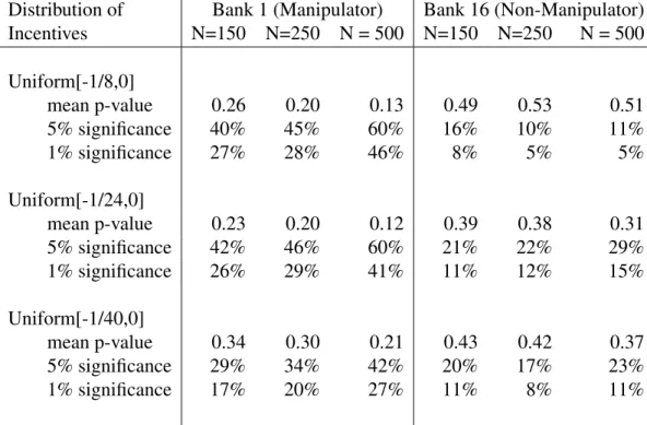
Table 1.1 shows the results of these experiments. Each entry in the table reports a summary statistic for the distribution of one sided t-test p-values obtained from simu-lating the model 1000 times for each associated parameterization. The hypothes tested is that the number of actual quotes, normalized by subtracting the day’s fourth lowest quote, falling in the bin 1 basis point below the fourth lowest ([−.01,0)) is less then the simulated number of normalized quotes falling into this bin.7 _{The rows in the table} 7_{We have run similar tests for an “Above” hypothesis that the number of normalized actual}

quotes falling in the bin 1bp above the fourth lowest is greater than the simulated number, and also a “Diff” hypothesis that the difference in the number of actual normalized quotes falling above and below is greater than the difference in the number of simulated normalized quotes.

(21)

report the average p-value, fraction of tests rejected at the 5% level, and the fraction of tests rejected at the 1% level and these are shown for a manipulator (Bank 1) and non-manipulator (Bank 16) for each of the parameterizations.

For each, simulation we maintain the assumption that there are 12 potential manip-ulators and bank costs are drawn from a joint normal distribution with mean 1 and covariance matrix equal to the empirical covariance matrix of 3 month Libor quotes less the daily mean quote.8 Across experiments we vary the sample size and two pa-rameters controlling the frequency of manipulation and the strength of manipulation incentives. The “Fraction of manipulating days” parameter determines the fraction of days on which there is potentially any manipulation so a parameter value of .33 means that on 2/3 of days no banks have any manipulation incentives (vi

8δ = 0,∀i). On days in which manipulation is possible the strength of manipulation incentives are determined by the “Distribution of Incentives” parameter. On these days each of the 12 banks re-ceives an incentive, vi

8δ, drawn iid across banks and days, from a mixture distribution with a 50% probability of getting a 0 draw and 50% probability of getting a draw from the uniform[−x,0]distribution, wherexis either 1/8, 1/24, or 1/40.

A first observation about the table is that each of the tests, evidently, allow us to dis-tinguish the manipulating bank from the non-manipulator. On average, the distribution of manipulator quotes will have less mass, relative to the comparison distribution, just below the pivotal quote. A manipulator will also have more mass just above and a greater difference in the mass just above and just below. The “Above” and “Diff” tests appear to do a much better job both of identifying the manipulator and distinguishing the manipulator from the non-manipulator than does the ”Below” test. However, un-like the former two the apparent ability of the “Below” test to contrast the two types

They give similar results

8_{Assuming that fewer banks are potential manipulators makes it easier to distiguish the}

manipulator from the manipulator since there are more cost events that lead to a manipulator being bunched at the lower pivot. For example, with only one manipulator a non-manipulating bank will only be bunched at the lower pivot in the event that the non-manipulator receives the fourth highest cost draw and the cost and incentives draw of the manipulator causes it to misreport at the same level as the non-manipulator.

(22)

improves, in the sense that the probability of incorrectly rejecting the null decreases for the manipulator while the probability of correctly rejecting the null for the manipulator improves for the “Below” test, whereas the other two tests increase the probability of correctly rejecting for the manipulator but also increase the probability of incorrectly rejecting for the non-manipulator.

Since our cost parameterization comes directly from the data, the table is also infor-mative about the relationship between test statistics and the underlying frequency and intensity of manipulation. When manipulation is less frequent and/or incentives are weaker, the tests in summarized in the table have low power, only rejecting the null of no manipulation at the 5% level in 50-60% of those samples with 150 or 250 observa-tions for the bottom rows of the table where the frequency and strength of manipulation is lowest. The simulated libor in this scenario is, on average .22 bp lower than what would prevail with honest reporting. By contrast, in the parameterization in the top rows of the table, where the null is correctly rejected for a manipulating bank at the 5% level 97-100% of the time, the average realized libor is .83 bp lower than what would prevail with honest reporting. These magnitudes suggest two things. First, our tests are able to detect deviations that are relatively small, when compared to day to day changes in quotes for instance, on average. Second, they suggest a ballpark lower bound on the frequency and intensity of manipulation incentives that we might infer from the strong rejection evidence we find our empirical analysis.

1.4 Data and Empirical Evidence

Our empirical analysis utilizes only data on bank rate submissions. The quotes of each panel bank on every business day from January 1, 2005 to July 1, 2012 were collected from a Bloomberg terminal. We focus on 3 month Dollar Libor submissions over the period ending February 1, 2011 when the panel increased to 21 members. From January 1, 2005 to February 1, 2011 the panel consisted the same 16 members with the exception of one change occurring in February 2009 when Societe General

(23)

replaced HBOS following the absorption of HBOS by Lloyd’s. Motivated by a visual examination of the Eurodollar bid rate-Libor spread shown in Figure 1.1 we split the sample up into 6 periods and perform our analysis on the full sample as well as on each period individually.

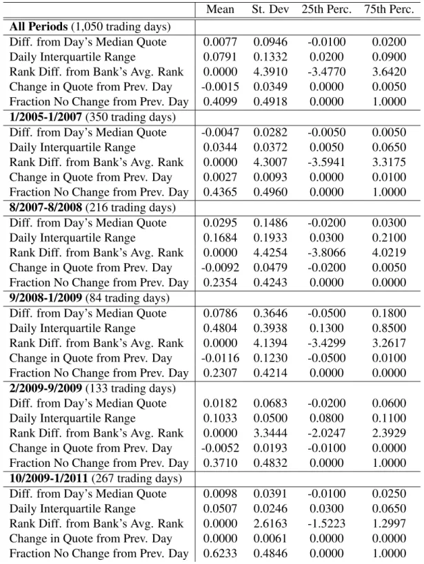
Table 1.2 shows some summary statistics for this sample over the various periods. On average, quotes are tightly clustered with an interquartile range of deviations from the median quote ranging from one basis point below to two basis points below. Similarly the interquartile range, the difference between the upper and lower pivotal quotes is quite narrow. Overall, the average size of the range is 7.9 bps, though there is a good deal of variation across our periods, with the range varying from 3.4 bps in the first year and a half of the sample to 48bps in the period containing the Lehman failure. Also notable is that, while the ranking of banks in the panel tends to be persistent, there is still considerable variation in relative ranks over time with the daily standard deviation of a bank’s rank from its average rank at 4.39. Moreover, nearly all banks occupy almost all ranks over a sufficiently long horizon. Significant variation in these relative quotes will be important for our testing strategy below.

As noted by Gensler (2012), one of the puzzling features of bank quote behavior is the lack of day to day movement in the submissions. Across all periods and all banks, over 40% of observations show no change from the previous day’s quote in spite of significant day to day changes in related rates. An interesting regime change seems to appear in the last 15 months of the summarized sample the number of such zeros jumps to 62% of observations. The lack of comovement of quotes with underlying “cost drivers” (as well as the lack of much movement at all) is the logic behind the collusion tests examined in Abrates Metz et. al (2012).

1.4.1 Empirical Approach

Our model predicts that when banks have direct incentive to manipulate rates, as op-posed to misreporting for other reasons, e.g. reputation, their quotes will bunch around

(24)

the pivotal quotes. Without placing restrictions on the joint distribution of bank quotes over time, obviously any distribution of quotes can be rationalized as truthful by some joint distribution of underlying costs. However, since different distributions will natu-rally display different degrees of bunching around the twelfth and fourth order statistics, any test will be sensitive to these restrictions. In trying to balance these trade-offs, we start by assuming latent underlying borrowing costs follow a vector autoregressive pro-cess.

ct=β0 +

X

Γτct−τ +εt

Where εt ∼ N(0,Σ).The VAR specification is a reasonably flexible way to describe time series relationships, however, there are two main restrictions embodied by this assumption. First, we assume that, in the long run, bank borrowing costs are correlated through similarities in the banks themselves. It is natural to think, for example, that U.S. based banks should have positively correlated costs or that all banks with large retail operations should be correlated. The crucial contrast here is that we rule out long run relationships between a bank’s borrowing costs and the borrowing cost of the fourth, or any other, rank bank. Second, is the assumptions that innovations are joint normally distributed. While the parametric restriction is necessary given the high dimension of the vector process, it is also undesirable. In the implementation of our tests, this is not directly an issue since, as discussed below, we work with fitted quotes.

Under a null of truthful reporting we can estimate this process using observed quotes. Due to cointegration and the high dimension of the vector process our preferred speci-fication is a two lag, rank two, vector error correction model.

∆qt = Πqt+

X

Λτ∆qt−τ +εt

With these estimates at hand we can examine how differences in the fitted or simulated versus actual distribution of quotes support our theory of manipulation (as opposed to simple misspecification of the cost process). Essentially, our testing strategy is to look

(25)

for statistically and economically significant differences in the distribution of prediction errors conditional on the position of pivotal quotes. Economically significant, here, means consistent with our model, which predicts a particular form of bunching and not others that might predict clustering of quotes together.9 _{Identification comes from} transitory changes in the relative bank ranks driven by actual idiosyncratic cost shocks or changes in misreporting incentives. For example, suppose JP Morgan and Citigroup are on average the fourth and fifth ranked banks and their quotes are highly correlated. If neither bank faces idiosyncratic shocks that drive them up or down in relative rank then, in the intraday distribution of quotes, both banks will be bunched at the fourth highest. The fitted model would reflect this and the fitted and simulated quotes of the two banks will also be bunched. If, on the other hand, occasional shocks shuffle JP Morgan out of the fourth rank and Citigroup’s submissions continue to bunch with the new occupant of the fourth spot, this will lead to bunching in the actual distribution but not the fitted and simulated distributions.

It is important to note that, if manipulation is present, our model will be contaminated even if our cost specification is correct. Thus, if the null of truthful reporting is false our comparison distribution should be expected to, itself, bunch more around the pivotal quotes than the actual cost distribution as in figure 1.3. How much more will depend on the degree of contamination; how many and how often banks are manipulating. Even if banks are constantly manipulating, however, the contaminated model will not display the predicted discontinuity in the distribution at the pivotal quotes. For this reason, we focus most of our attention on this discontinuity.

1.4.2 Results

Figure 1.4 (Figure 1.5) shows the pooled distribution of quotes of all banks normalized by subtracting the fourth (12th) highest quote of the 15 other bank quotes over vari-ous time periods. The bottom half of each panel show the fitted versions of the same 9_{Banks may cluster together if they all have incentives to simply not stick their “heads above}

(26)

normalized quotes.10 We use fitted quotes for our comparison distribution rather than simulating innovations and adding them to the fitted quotes because we worry about non-normality of the quotes. In particular, the large number of no-change observations suggests that the fitted quotes may be a better choice. We have performed the same analysis using simulated quotes as well and it only strengthens the results.

A couple of features of these figures stand out. First, to a striking degree the distri-butions resemble the shape predicted by our model for both the upper and lower pivot normalizations. Second, the distribution of normalized fitted quotes also displays a good deal of bunching around the pivotal quotes, demonstrating the importance of de-veloping our benchmark comparison distribution. To statistically verify this graphical story we implement some simple statistical tests, motivated by the numerical experi-ments with the model. Namely, we test for a discontinuity in the quote distribution at the pivotal quote. A natural approach for such a discontinuity test is suggested by Mc-Crary (2008). Unfortunately rounding of quotes combined with the small scale make the required smoothing impossible so instead we simply compare the histogram bin size of a small interval,[0, b)((0, b]), above the quote minus the fourth (twelfth) highest to the bin size of a small interval, [−b,0)((−b,0]), below the quote minus the fourth (twelfth) highest. Since 65% of quotes are rounded to the nearest basis point, an ad-ditional 25% are rounded to the half basis point, and most of the rest are rounded to the quarter basis point, our preferred window size is one basis point (b = .01) but we report many of our results for the half (b =.005)and two(b =.02) basis point levels as well.

Tables 1.3 show the results of our “Lower” bunching tests for all banks pooled together at various window widths.11 _{The table confirms the graphical evidence. For almost} all periods and window widths each of our three bunching tests are significant at the 1% level for the lower pivot normalization. The only exception is in the final period from October 2009 to January 2011 with 1bp window width. Here, the probability of a 10_{That is, for each bank, we subtract the fourth (12th) highest of the 15 other}_fitted _quotes

from its own fitted quote.

11_{Bank level histograms are available on the authors’ website. “The Fix is In: Additional}

(27)

normalized quote falling in the bin just below zero is almost identical for the fitted and actual distributions. The prevalence of zero-change days, no doubt, contributes to an overall similarity in the fitted (zero innovation vector) and actual quotes.

For the whole basis point windows, notably, the total mass in the windows around zero are similar for the fitted and actual distributions. Examining the data a bit more closely shows why this is the case. A huge fraction of quotes predicted to fall into the bin just below (just above in the case of the upper pivotal quote normalization) zero, fall into the just above (just below) bin. This demonstrates the mechanics of our tests using the possibly contaminated estimates as a benchmark distribution. If the comparison distribution were the actual distribution of costs we would expect to see quotes moving from bins further above (below) the pivots to bins closer to the pivots. Our tests are instead exploiting the change in the shape of the distributions at the pivotal quotes. Table 3c-d delve into the tests with two way tables showing the joint distribution of fitted and actual normalized quotes pooled over all banks and periods. In the analysis of individual banks, almost all bank-periods that fail our test have this same pattern.

1.4.3 The Timing of Bunching and Collusion

Reports from ongoing Libor investigations and media coverage have indicated likely collusion among panel banks in manipulating rates. The basic implications, in terms of the shape of the intraday distribution of quotes, from our model are unchanged in the presence of collusion. When banks collude, however, the scope for manipulation is much greater and thus has serious implications for the magnitude of manipulation and resultant welfare effects. When a bank acts unilaterally, their ability to distort the rate down, relative to the rate that would prevail from honest reporting, is bounded by 1/8 times the difference between its true cost and its submission. At the other extreme, five or more banks acting in concert move the rate as far as they desired, though in a collusive equilibrium of our model they will not choose to do so due to the convex misreporting costs. To explore collusion in light of our model we simply extend our bunching tests to look at the correlation between banks of bunching behavior over time.

(28)

We leave a fuller development of tests for collusion to future work.

Figures 1.6 and 1.7 show the results of redoing our main bunching analysis using a rolling window rather than pooling within discrete periods for 3M and 6M tenors for the dollar Libor. Specifically we calculate kernel smoothed frequency of quotes falling into either the 1bp above the pivot or 1bp below the pivot

Y_i,ta,4 = T P τ=1 K(t−τ_h )1{0≤qit−s4 < b} T P τ=1 K(t−τ_h ) Y_i,tb,4 = T P τ=1 K(t−τ_h )1{−b ≤qit−s4 <0} T P τ=1 K(t−τ_h )

Where we use a simple, triangular kernel with 10 day bandwidth for K. We calcu-late the corresponding smoothed measure for quotes normalized by the twelfth highest quote and compare these with the fitted versions of the same.

There is no obviously strong pattern of correlation in bunching behavior in these mea-sures between banks, though visually there appears to be a loose correlation in the timing of bunching episodes across all banks. The graphs also support the general ob-servation that bunching declines in the periods immediately following the failure of Lehman Brothers and the depths of the financial crisis, incidentally the time when it is most likely that reputation driven manipulation was occurring. This is especially true of the upward manipulation tests.

The picture painted here generally corroborates the discussion above. While there ap-pears to be some correlation across banks in their bunching behavior, the correlations are as consistent with the existence of common underlying drivers of manipulation, as in the example of future positions, as they are with an explicit conspiracy. Moreover,

(29)

since different sets of banks appear to be pushing in opposite directions at the same time and these sets don’t appear to be stable, the evidence is not suggestive of any specific set of banks participating in a grand cartel. In general, the data appear consistent with uncoordinated episodic manipulation, which may have involved occasional cooperation among multiple banks.

1.5 Conclusion

Over the past 30 years most corners of financial markets have come to rely on Libor as an essential gauge of the health of money markets and the direct and indirect implica-tions thereof. Such heavy dependence has made the recent revelaimplica-tions of widespread manipulation of these rates shocking to the point of crisis. Concerns about manipula-tion were originally focused on the most tumultuous period of the financial crisis, when, it was suggested, banks may have been understating their borrowing costs in order to avoid negative market (over)reaction. While such a suggestion was disconcerting, mar-ket observers could take solace in the fact that the problems with the rate were confined to times when nothing seemed to be working properly and in the fact that misreporting banks may have been doing a public service by helping avoid further panic. Recently, however, investigations by regulators have uncovered evidence of manipulation driven by bank trading positions with exposure to Libor.

In this paper we have developed tests for portfolio driven manipulation based on a model of Libor panel bank survey submissions. The model predicts that the intraday distribution of panel bank quotes will bunch around the fourth (twelfth) highest quote in the presence of incentives to push the rate down (up). Our simple tests are designed to deal with a couple of the most important empirical challenges presented by the sub-missions data and alternative indicators of manipulation. Since we do not have a strong prior on the form of the joint distribution of interbank borrowing costs, we develop a flexible benchmark distribution with which to compare the actual quote distribution. Our benchmark distribution is constructed by estimating a VAR model of bank quotes,

(30)

which imposes that long run cost correlations are related to similarities between the banks themselves but unrelated to the rank of any bank per se. We also take steps to ensure our testing procedure is robust to the rounding and infrequent quote changes found in the data.

Going to the data, we find strong evidence of the type of bunching predicted by our model. Concerns about false negatives and false positives associated with our tests notwithstanding, the bunching evidence is especially strong in the early periods of our sample, with almost every bank individually failing our bunching tests at a very high level of significance. Aspects of our findings are consistent with accounts of collusive behavior, however, they are also consistent with common underlying sources of manip-ulation incentives such as futures reset dates. Also, consistent with publicly available accounts of manipulation, our evidence suggests that coordination between particular banks was, if anything, on an episode by episode basis as opposed to a more centralized, overarching conspiracy.

One limitation of our analysis is that it requires pooling of quotes over time, making pinpointing specific, suspicious observations difficult. However, we are able to per-form our tests at the bank level and at more coarse time breakdown enabling the tests to inform a coherent narrative. Another limitation of our study is that we have not done much to quantify the degree of manipulation. The best we can offer is evidence from numerical simulations of our model. Viewed as back of the envelope calculations, these results suggest test rejections at the level we observe, indicate frequent manip-ulation and strong incentives with an average deviation of observed Libor rates from actual rates over .5bp, which amounts to over a trillion dollars of contract mispricing on aggregate.

Our analysis has several implications for the effective reform of Libor, several of which have already been adopted by the Wheatly commission. One of these is the desirability of putting more banks on the panel. As the number of banks increases, the influence of any one bank on the overall rate diminishes and thus so do the incentives for misre-porting. Our model also suggest increased regulatory oversight and audited submission rules would also be desirable as these increase misreporting costs. The Wheatly

(31)

Com-mission opted not to adopt the change, suggested by some, to make subCom-missions anony-mous instead embargoing quote data for 60 days after submission. Our results suggest this is likely a sensible middle ground. Total anonymity might decrease misreporting costs for panel banks. On the other hand, total visibility increases the likelihood of tacit collusion.

(32)

Table 1.1: Monte Carlo of Test on Model Simulated Data

Distribution of Bank 1 (Manipulator) Bank 16 (Non-Manipulator) Incentives N=150 N=250 N = 500 N=150 N=250 N = 500 Uniform[-1/8,0] mean p-value 0.26 0.20 0.13 0.49 0.53 0.51 5% significance 40% 45% 60% 16% 10% 11% 1% significance 27% 28% 46% 8% 5% 5% Uniform[-1/24,0] mean p-value 0.23 0.20 0.12 0.39 0.38 0.31 5% significance 42% 46% 60% 21% 22% 29% 1% significance 26% 29% 41% 11% 12% 15% Uniform[-1/40,0] mean p-value 0.34 0.30 0.21 0.43 0.42 0.37 5% significance 29% 34% 42% 20% 17% 23% 1% significance 17% 20% 27% 11% 8% 11%

Data simulated using various parametizations of the complete information static game presented in the paper. Statistics calculated from 10,000 runs of N sample days of simulated data. In each run 12 banks are manipulator banks which means they occasionally have incentives (v ≥0) to manipulate.

(33)

Table 1.2: Three Month Dollar Libor Summary Statistics

Mean St. Dev 25th Perc. 75th Perc. All Periods(1,050 trading days)

Diff. from Day’s Median Quote 0.0077 0.0946 -0.0100 0.0200 Daily Interquartile Range 0.0791 0.1332 0.0200 0.0900 Rank Diff. from Bank’s Avg. Rank 0.0000 4.3910 -3.4770 3.6420 Change in Quote from Prev. Day -0.0015 0.0349 0.0000 0.0050 Fraction No Change from Prev. Day 0.4099 0.4918 0.0000 1.0000 1/2005-1/2007(350 trading days)

Diff. from Day’s Median Quote -0.0047 0.0282 -0.0050 0.0050 Daily Interquartile Range 0.0344 0.0372 0.0050 0.0650 Rank Diff. from Bank’s Avg. Rank 0.0000 4.3007 -3.5941 3.3175 Change in Quote from Prev. Day 0.0027 0.0093 0.0000 0.0100 Fraction No Change from Prev. Day 0.4365 0.4960 0.0000 1.0000 8/2007-8/2008(216 trading days)

Diff. from Day’s Median Quote 0.0295 0.1486 -0.0200 0.0300 Daily Interquartile Range 0.1684 0.1933 0.0300 0.2100 Rank Diff. from Bank’s Avg. Rank 0.0000 4.4254 -3.8066 4.0219 Change in Quote from Prev. Day -0.0092 0.0479 -0.0200 0.0050 Fraction No Change from Prev. Day 0.2354 0.4243 0.0000 0.0000 9/2008-1/2009(84 trading days)

Diff. from Day’s Median Quote 0.0098 0.0391 -0.0100 0.0250 Daily Interquartile Range 0.0507 0.0246 0.0300 0.0650 Rank Diff. from Bank’s Avg. Rank 0.0000 2.6163 -1.5223 1.2997 Change in Quote from Prev. Day 0.0000 0.0061 0.0000 0.0000 Fraction No Change from Prev. Day 0.6233 0.4846 0.0000 1.0000

(34)

Table 1.3: All Bank Bunching at the 4th Lowest Quote (3M Dollar) Window q−s4 All 1/2005- 8/2007- 9/2008- 2/2009- 10/2009-Periods 7/2007 8/2008 1/2009 9/2009 1/2011 b = .005 Actual 0.029 0.042 0.018 0.005 0.013 0.036 Simulat. 0.067 0.106 0.046 0.022 0.040 0.059 p-value 0.000 0.000 0.000 0.000 0.000 0.000 b = .01 Actual 0.071 0.067 0.055 0.023 0.062 0.107 Simulat. 0.105 0.141 0.083 0.040 0.078 0.108 p-value 0.000 0.000 0.000 0.000 0.001 0.365 b = .015 Actual 0.089 0.089 0.078 0.032 0.073 0.126 Simulat. 0.133 0.159 0.113 0.051 0.107 0.152 p-value 0.000 0.000 0.000 0.000 0.000 0.000 b = .02 Actual 0.117 0.103 0.111 0.053 0.107 0.164 Simulat. 0.154 0.171 0.136 0.070 0.129 0.184 p-value 0.000 0.000 0.000 0.001 0.000 0.000

(35)

Figure 1.1: Libor -Eurodollar Bid Rate (1/2005-7/2012)

(36)

Figure 1.2: Costs vs. Quotes in Model of Manipulation

(37)

Figure 1.3: Simulated Distrib ution of Quotes Minus Daily 4th Lo west of 15 Other Banks

(38)

Figure 1.4: All Banks: 3M Bank Quote Minus the 4th Lo west of Fifteen Other Banks

(39)

Figure 1.5: All Banks: 3M Bank Quote Minus the 4th Highest of Fifteen Other Banks

(40)

Figure 1.6: All Banks: 3M Dollar Rolling Bunching T est

(41)

Figure 1.7: All Banks: 6M Dollar Rolling Bunching T est

(42)

Chapter 2

(43)

2.1 Introduction

Trader:[Would] be nice if you could put 0.90% for 1mth cheers.

Quote Submitter: Sure no prob. I’ll probably get a few phone calls but no worries mate!

Trader:If you may get a few phone calls then put 0.88% then.

Quote Submitter: Don’t worry mate – there’s bigger crooks in the market than us guys!

—Rabobank, internal discussion1 The Libor was recently subjected to one of the largest instances of market manipulation in history. Hundreds of trillions of dollars worth of financial contracts were manipulated by large banks, who have since been fined billions of dollars by regulators from four countries.2 _{Investigations are ongoing and many class action lawsuits are underway due} to the huge volume of contracts adversely affected.3

The banks under investigation had simple incentives: they owned contracts whose pay-outs were functions of the Libor. While recent regulatory investigations have revealed that these portfolio incentives did in fact lead to manipulation, it is not known how this affected the overall Libor rate. It is possible the Libor remained largely unchanged throughout this episode, either due to an inability of banks to consistently execute ma-nipulative intent, or thanks to varying portfolio incentives across banks. On the other hand, manipulation may have caused a systemic distortion, which would undermine the

1_{From the Department of Justice’s investigation of Rabobank, see (DOJ (2013))}

2_{Wheatley (2012) estimates $300 trillion worth of contracts directly reference the Libor}

when determining interest rate payments. The regulatory bodies of the USA, UK, Switzer-land, and the Netherlands have variously fined Barclays, UBS, the Royal Bank of Scotland and Rabobank.

3_{The city of Baltimore, New Britain Firefighter’s and Police Benefit Fund,}

At-lantic trading USA, and Community Bank&Trust are some of the representative mem-bers of the four classes pursuing Libor related damages, according to Perkins Coie (http://www.perkinscoie.com/libor faqs/). See Dodd (2010) for a description of the losses incurred by municipalities.

(44)

continued value of the Libor as a benchmark. Any persistent distortion may have af-fected the allocation of funding in this period, as an estimated $10 trillion of syndicated loans use the Libor as the variable interest rate (Wheatley (2012)).

In this paper, I quantify the degree to which manipulation distorted the Libor between 2005 and 2009. To do so, I estimate a strategic model where the Libor is formed each day in a noncooperative game of incomplete information. The strategic interaction between banks is generated by the aggregation mechanism of the Libor survey. Of the sixteen quoted rates, only the middle eight quotes are used in the resulting average which determines the benchmark. The four highest and lowest quotes are discarded. This means, if a bank was a manipulator, it would need to forecast the quotes of its peers in order to gauge its marginal ability to influence the overall Libor rate. Variation in this marginal ability across banks and trading days allows me to recover each bank’s average portfolio exposure to the Libor and, consequently, what they would have quoted had they had no such exposure.4

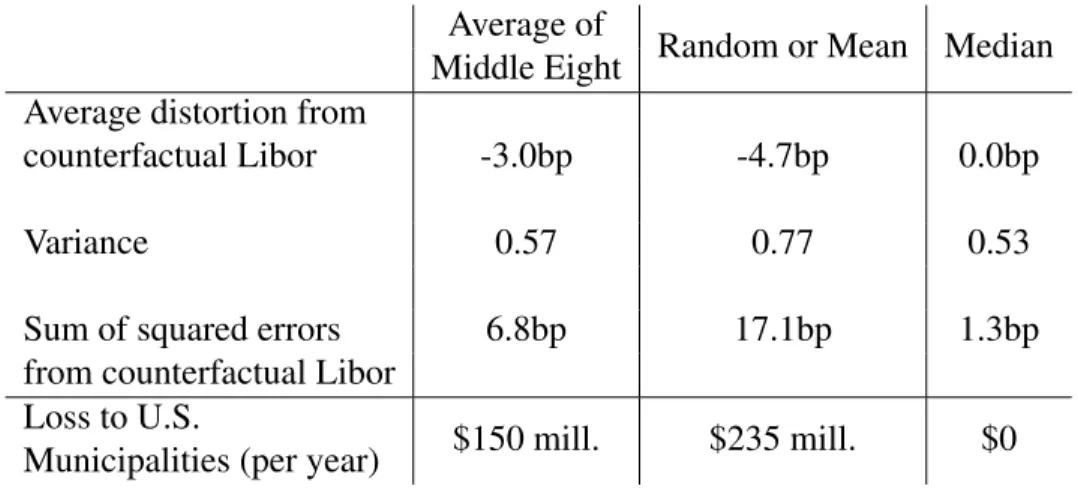
I find that the Libor was largely accurate prior to the financial crisis starting in late 2007, but was since distorted downwards by eight basis points. This is substantial given the volume of contracts affected and that manipulators routinely made large gains from single basis point changes.5 I calculate that U.S municipalities, which held $500 billion worth of interest rate swaps in 2010, would have lost $455 million from this eight basis point shift over my sample period.6

4_{There are many other benchmark interest rates similar to the Libor, including the}

Tokyo-based Tibor, the Mumbai-Tokyo-based Mibor, the many Euribor, and others. Since these are also typically calculated using truncated averages, the strategy I employ in this paper could be used to study the manipulation of these benchmarks as well.

5_{This is a common theme in the regulatory investigations. See for example FCA (2012a):}

“Barclays’ Derivatives Traders knew on any particular day what their books’ exposure to a one basis point (0.01%) movement in Libor or Euribor was.” A Barclays trader said to the quote submitter, “We have about 80 [billion] fixing for the desk and each [basis point] lower in the fix is a huge help for us.” (Ibid.) See also FCA (2012b) and Snider and Youle (2012) for more examples.

6_{See Preston (2012) and Dodd (2010) for background on municipal ownership of}

(45)

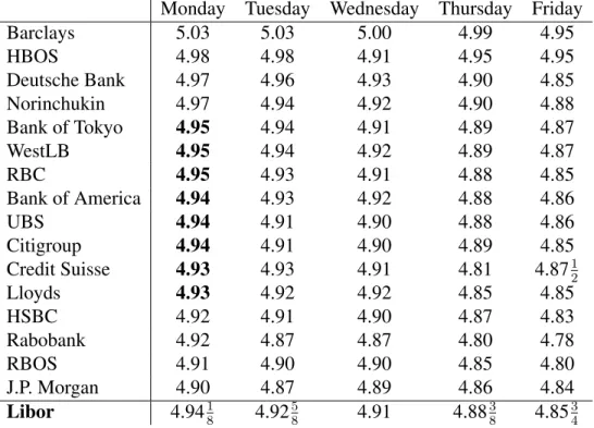
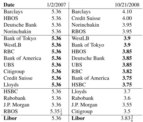
The transition between an accurate pre-crisis Libor and a distorted post-crisis Libor was driven by sharp changes in volatility and heterogeneity across banks. Prior to the finan-cial crisis, banks had very similar risk characteristics and typically submitted identical or near-identical quotes to the survey. If the other fifteen banks are all submitting the same, correct rate, what could a potential manipulator achieve by submitting something different? Once the crisis began, however, banks’ faced newly heterogeneous risks and submitted a broader range of quotes to the survey. This generated a larger interquartile range between the fifth and twelfth highest submissions which gave potential manipu-lators room in which to work.

With these results in mind, I compare the performance of counterfactual Libor aggre-gation mechanisms in the presence of active manipulators. This contribution is partic-ularly timely as regulators are currently considering how best to reform to the Libor to safeguard it against future manipulation.7 In particular, the Financial Conduct Author-ity (FCA) is considering increasing the size of the Libor panel, anonymizing quotes for three months, and tying quotes to underlying transactions as much as possible.8 While the FCA also considered changing the current mechanism used to calculate the Libor from the underlying quotes, they concluded this would not improve the Libor’s accuracy.

I find, on the contrary, that changing the current mechanism for calculating the Libor can make it considerably less vulnerable to manipulation. In particular, changing the Libor to use the median quote removes virtually all of its systematic downwards bias in the sample period I examine. My results differ from those of the FCA analysis because they assume submitted quotes would not change even if the method used to calculate the Libor were changed. This runs contrary to the idea that manipulators take into account the aggregation mechanism when they strategically submit their quotes. Documents revealed by the investigations show manipulators had a very keen awareness of the exact mechanism.9 In my counterfactual analysis, manipulators are perfectly aware of

7_{The Libor and other benchmarks are becoming regulated for the first time.} 8_{See Wheatley (2012) for a comprehensive review of the FCA proposals.} 9_{See, for example, FCA (2012a)}

(46)

the aggregation mechanism when they submit their quotes.

The counterfactual performance of the median is driven by the difficultly for manip-ulators to accurately forecast the location of the median on any given day. Even if a manipulator were able to correctly guess the median, they would not be able to skew their quote very far before they were no longer the median submission. In essence, using the median is similar to narrowing the interquartile range. There could also be a feedback effect. If the median mechanism causes most other banks to skew less, manipulators may skew less as they update their median forecasts.

For some values of the model parameters, however, the median can actually perform worse. The is because the distribution of private information plays an important role in my model’s equilibrium. The performance of the median, relative to the interquartile range, depends on this distribution as well as the incentives for banks to manipulate. In particular, under certain conditions, a manipulator may be more or less certain they will be the median quote. In this case, the median mechanism would give them much greater power in determining the final rate, which lead the manipulator to skew more than they would otherwise.10 _{This ambiguity is why I must bring the model to the data.} I model banks in the Libor panel as playing a noncooperative game of incomplete in-formation. Each bank has a true interbank borrowing cost which depends on publicly observed covariates, as well as an idiosyncratic shock which is private information. Each bank is therefore uncertain of the quotes of the other banks when submitting its own quote. Manipulators are concerned with the quotes of the others because they want to forecast the interquartile range within which they can affect the Libor. Banks that aren’t manipulators, however, are not concerned with forecasting the quotes of their peers.

My game is estimated in two steps. First, I nonparametrically estimate each bank’s marginal impact on the expected Libor. This marginal impact is an equilibrium object 10_{Diehl (2013) shows the relative performance of the median-quote Libor is ambiguous in a}

complete information version of the game introduced in Snider and Youle (2012). This ambi-guity persists in my current, incomplete information game.

(47)

which depends upon the strategies being played by the other banks. In the second step, I form moments from the model’s first order conditions and use the submitted quotes and the results from the first step to estimate the game’s parameters, which include banks’ incentives to manipulate. From this, I construct a “manipulation free” Libor by calculating what banks would have quoted had they had no such incentives.

It is important to note that portfolio exposure to the Libor was not the only reason banks submitted misleading quotes. The other reason was reputational. Each bank’s quote is publicly revealed after the Libor is computed. Whenever a bank submits a relatively high quote, thereby admitting to a high cost of borrowing funds from its peers, other market participants might infer something is amiss with that bank. In the run-prone environment of the recent financial crisis, it is unsurprising that banks wished to avoid this negative attention. Indeed, regulators have uncovered many documents expressing banks’ desires to avoid being seen as lacking creditworthiness.11

I do not attempt to meaningfully capture these reputational incentives for banks to sub-mit misleading quotes. Instead, I control for them with a flexible specification of fixed effects. I use bank-quarter effects and use the within-bank, within-quarter variation in marginal impacts upon the Libor to identify my model. Reputational effects are im-plicitly incorporated into my counterfactual analysis and the manipulation-free quotes I produce. I do not recover the “correct” Libor, only a Libor free of portfolio-driven ma-nipulation.12 These reputational incentives to misreport will be reduced by the FCA’s new policy of anonymizing individual quotes fir three months. This anonymity, how-ever, will exacerbate banks’ portfolio-driven incentives to misreport by reducing the ability of other market participants to examine and monitor the submitted quotes. Snider and Youle (2012) use a similar model to motivate a test for Libor manipulation. My approach differs from theirs by assuming banks play a game of incomplete infor-mation. This relatively minor modeling difference leads to a completely different em-pirical strategy. Incomplete information creates smoothness in banks’ profit functions and allows the derivation of a system of necessary first order conditions. Estimating

11_Ibid.

(48)

these first order conditions lets me measure the sizeof banks’ long term average ex-posures to the Libor. Knowing this size allows me quantify the extent of the Libor’s distortion and examine the accuracy of counterfactual aggregation mechanisms. I am unable, however, to capture manipulation that occurs at a high frequency, which was an important part of the Libor’s recent manipulation, and for which Snider and Youle (2012)’s test is better suited to detect.

This paper is related to the recent literature on estimating games that occur in financial markets. Cassola et al. (2013) measures banks’ demand for funding through a structural auction model of the EONIA funds service. They use observed bids and the structure of the auction to recover banks’ valuations. In my model, I use observed quotes and the structure of the Libor mechanism to recover banks’ portfolio exposures. Guerre et al. (2009) use an exclusion restriction in an auction setting to separately identify bid-ders’ risk aversion from their distribution of valuations. I also employ an exclusion re-striction to separately identify manipulators’ portfolio exposures from their unobserved interbank shocks.

The rest of the paper is structured as follows. Section 2 describes the history of the Libor and the recent manipulation scandal. Section 3 describes my data. Section 4 introduces the strategic model of manipulation. Section 5 describes my estimation pro-cedure and results. Section 6 discusses my results. Section 7 introduces an algorithm to compute the Bayes-Nash equilibrium and compares counterfactual Libor mechanisms. Section 8 concludes.

2.2 History of the Libor

The London Interbank Offered Rate (Libor) is a benchmark interest rate that has grown to become a central institution in financial markets.13 An estimated $300 trillion of 13_{The Libor is quoted in many different maturities and currencies. In this paper I focus on}

the three month dollar Libor which, along with the six month Libor, is most commonly used by financial contracts.