Zhao, W
and
Beach, TH
and
Rezgui, Y
(2017)Efficient least angle
regres-sion for identification of linear-in-the-parameters models.
Proceedings of
the Royal Society A: Mathematical, Physical and Engineering Sciences, 473
(2198). ISSN 1364-5021
Downloaded from:
http://e-space.mmu.ac.uk/622663/
Version:
Accepted Version
Publisher:
The Royal Society
DOI:
https://doi.org/10.1098/rspa.2016.0775
Please cite the published version
Efficient least angle
regression for identification
of linear-in-the-parameters
models
Wanqing Zhao, Thomas H. Beach and
Yacine Rezgui
Least angle regression (LAR), as a promising model selection method, differentiates itself from convent-ional stepwise and stagewise methods, in that it is neither too greedy nor too slow. It is closely related to L1 norm optimisation, which has the advantage of low prediction variance through sacrificing part of model bias property in order to enhance model generalisation capability. In this paper, we propose an efficient least angle regression algorithm (ELAR) for model selection for a large class of linear-in-the-par-ameters (LIP) models with the purpose of accelerating the model selection process. The entire algorithm works completely in a recursive manner, where the correlations between model terms and residuals, the evolving directions and other pertinent variables are derived explicitly and updated successively at every subset selection step. The model coefficients are only computed when the algorithm finishes. The direct involvement of matrix inversions is thereby relieved. A detailed computational complexity analysis indicates that the proposed algorithm possesses significant computational efficiency, compared to the original approach where the well-known efficient Cholesky decomposition is involved in solving least angle regression. Three artificial and real-world examples are employed to demonstrate the effectiveness, efficiency and numerical stability of the proposed algorithm.
1. Introduction
Research into a large class of linear-in-the-parameters (LIP) models for nonlinear system identification has con-sistently drawn substantial interest from both academic and industrial communities [1–6], making it an important
research topic in the field of computational intelligence and machine learning. The main reason can be attributed to the fact that a variety of conventional and advanced models, networks or systems, such as polynomial models [7–9], RBF (radial basis function) neural networks [10–12], fuzzy rule-based systems [13–15] and least-squares support vector machines [16–18], can somehow be treated and trained as LIP models. The essential concept of LIP models is that they are formed by a set of linearly combinatorial model terms which are in turn nonlinearly mapped from the original model input space. For instance, a fuzzy system can be viewed as a series of linear expansion of fuzzy basis functions transformed from a model input space [13], where the claimed interpretability virtue lies in explaining the developed fuzzy system in terms of understandable IF-THEN linguistic rules, where the rule premises are employed to partition the input space into fuzzy regions in which the rule consequents are valid to describe the system’s behaviour. The model terms in LIP models are also recognised as, or closely related to some well-known terminologies, e.g., monomials, basis functions, hidden nodes, fuzzy rules and support vectors, in various research contexts. Here, except for polynomial models, nonlinear parameters are often involved in the model terms for mapping the original model space into another hyperspace in order to improve model performance.
Although LIP models are widely considered to have strong approximation abilities given a complex enough model structure, challenging scientific problems arise in how to effectively and efficiently determine a proper model structure and the associated parameters, a process which is often known as model selection (aka subset selection). A simpler model structure with fewer model terms included is usually preferred from several perspectives, such as model interpretability, model sparsity and model generalisation capability. For example, a small number of fuzzy rules included in a fuzzy system would help understand the underlying system behaviours being described. Meanwhile, the associated unknown model parameters also need to be estimated. In practice, a large number of candidate model terms can usually be generated from measured data, from which the selection of a compact set of model terms that make up a LIP model with acceptable model performance is desirable. If an excessive number of model terms are adopted, an unnecessarily complex LIP model can thereby be resulted with deteriorated model interpretability and generalisation abilities.
Therefore, the model selection of LIP models aims to find a small subset of model terms for predicting system output with good accuracy. This is a very important research area and constitutes the main topic of the paper. Unsupervised learning methods are amongst earlier attempts for performing model selection, the well-known representatives being the clustering-based methods and rank-revealing or decomposition-clustering-based methods [19–24]. These methods are intrinsically fast as usually only data from input space is processed without explicitly considering the system output information. This inevitably leads to important difficulties, i.e., inaccurate models learnt from data, because feedback does not exist to assess model output using training data. It is noted though clustering methods may also employ output information in certain cases, but turning out that the corresponding computational complexities are dramatically increased and the connection of the obtained clusters to a particular LIP model is not always straightforward. Therefore, a refinement stage is required to further enhance model performance, where the so-called supervised learning is introduced. Consequently, research on accurate model selection methods is more focused on supervised learning methods.
Amongst supervised learning methods, obsolete approaches use exhaustive search to examine every size of possible combinations of model terms in the least-squares sense, which is computationally extremely expensive and even practically infeasible when a large number of terms are available [15]. Fortunately, the stepwise selection techniques [25] provide alternative approaches to significantly mitigate the computational burden at the expense of introducing locally optimal solutions. In the framework of forward stepwise selection, it performs the model selection sequentially, in that each step a new term is included into the model to maximumly improve model performance, where the model coefficients for a series of candidate models are normally computed in the least-squares sense. This means that the model residual vector obtained
after the inclusion of each new model term is always orthogonal to all the selected model terms. It still exhibits heavy computational burden behind the raw idea of the stepwise approach, as many candidate model terms and inverse operations are usually involved in the model selection process.
Nowadays, there are a few efficient model selection algorithms working on the forward stepwise principle though distinct model searching criteria are adopted. For example, despite different schemes used to deal with the involved inverse operations, the orthogonal least-squares (OLS) [26–30] and fast recursive algorithm (FRA) [3,31] were proposed to pursue the largest reduction ofL2norm of model residuals at every model selection step. Alternatively, the correlation between the model residual resulting from each step and the remaining unselected model terms can also be used as the searching criterion instead of the residual’sL2norm, where the candidate term giving the largest correlation is selected at the following step. In addition to the forward stepwise approaches, it may be worth mentioning that backward stepwise approaches [25] are similar techniques but working in a reverse manner (starting with the inclusion of all candidate model terms and then eliminating the most insignificant one at a time). However, the whole process can be inefficient, especially when a large number of candidate model terms are available.
It has been found that the forward stepwise approach performs greedy optimisation in the sense that each time the best model term is greedily (where the least-squares estimation is performed, resulting in the selected terms completely orthogonal to the model residual, i.e., zero correlation between them) added into the selected pool based on a number of previously chosen terms. Given this greedy optimisation methodology, it can normally find locally optimal solutions according to some searching criterion. Instead, the forward stagewise selection as a less greedy approach opposed to the forward stepwise [32,33], iteratively identifies the most correlated term with the current model residual and thereby only updates its own coefficient with an amount proportional to the corresponding correlation (but not equal to it, meaning a smaller optimisation step compared to stepwise) at each iteration step. As a result, the resultant correlation for the selected terms is non-zero and is decreased during the model selection process, until reaching zero and the least-squares solution is thus approached. The downside therefore lies in that the iterative working manner of this approach requires a large number of iteration steps (usually being considerably larger than the available number of model terms), incurring huge computational burden. It is worth noting that, to improve optimality and model generalisation performance, distinct enhancements have also been made to the forward stepwise methods based on either OLS or FRA, including the involvement of additional refinement phases (where the selected model terms are reviewed and replaced by unselected terms with larger contribution to the underlying model) and/or the regularisation techniques (where penalised cost functions are imposed on either the original or converted orthogonal space of the system) [15,34–37]. The model performance has since been greatly improved while a global optimality cannot be guaranteed, the computational burden being thereby increased due to the extra computing phases and/or (determination of) the introduced regularisation parameters.
As a trade-off between the aforementioned stepwise and stagewise approaches, the newly joined model selection approach, least angle regression (LAR) [25,32], provides another efficient model selection framework motivated from the geometrical perspective [38]. It has also been found that a direct modification of LAR can lead to the full-path of Lasso (Least absolute shrinkage and selection operator) solutions [25,32,39], whereL1regularised cost is adopted to minimise the sum of squared residuals (SSR) and theL1norm of model coefficients. LAR uses a similar working manner as in stepwise while adopts the concept behind stagewise, but the key idea instead is to decrease the correlation for the selected terms at each step at a reasonably large step size that just makes the correlation for the selected terms equal to the correlation for an unselected term. The correspondingly unselected term is then added into the model and the correlations are decreased equally amongst all the selected terms during the model selection process until reaching the least-squares estimation given all available terms selected. Differing
from the greedy selection employed in the stepwise approach and the iterative optimisation (indicating high computational demand) exhibited in the stagewise approach, LAR owns both less greedy merits and the efficient stepwise selection manner (indicating less computational demand). In this respect, it might be worth mentioning that theL2norm regularised optimisation (aka ridge regression) can also be used for shrinking model coefficients towards zeros. However, it is unable to force coefficients to exact zeros, in order to remove the corresponding model terms from the final model. Apart from working on linear regression models, it is interesting to note that, LAR (specifically its underpinning equiangularity condition) has also been generalised in a number of different settings. For instance, it was extended to generalised linear models [40] through considering the model’s differential geometrical structure. In addition, relating the correlation for various model terms to the corresponding gradient of the cost function under investigation, LAR has also recently been extended for applying on generalised linear/quasi-likelihood models [41], Cox’s proportional hazard models [42] and more generally any convex cost functions [38], where ordinary differential equations (ODEs) are successively solved to infer the corresponding solution path.
In particular, regarding the greediness of stepwise algorithms, such as OLS, theoretically, they lead to the resultant model residuals being always orthogonal to the selected model terms, which means that the terms are thoroughly added into the model at each step of model selection (i.e., giving the best modification at each single step irrespective of the future effect [43]). In principle, this mechanism is aggressive and can be overly greedy as useful terms which are correlated with selected ones are unlikely to be included into the model subsequently due to the low explanatory power given on the underlying model. In this regard, stagewise methods which partially add terms into the model at some small/tiny step size at each step can also be employed to understand the greedy behaviour exhibited by the forward stepwise method (being corresponded to that of a large enough step size used in stagewise). Since the stagewise method itself is computationally very slow due to the many tiny iterative optimisation steps, thus LAR was proposed to dramatically mitigate the computational demand with the correlation between selected terms and model residuals decreases in a reasonably fast manner determined algebraically. Simulations have also been designed and conducted to verify the above points by Efron et al. [32]. It had been found that, as the model size increases, the predictive model performance (goodness of fit) of LAR was able to rise reasonably quickly, then decrease very slowly after reaching some maximum value. In contrast, the model performance of forward stepwise method can rise and decline more sharply than that of LAR. In this sense, the generalisation performance of stepwise can be better than that of LAR at the beginning of model selection just due to its greedy nature, but as more model terms were then subsequently included into the model, the situation was gradually reversed. The generalisation performance of LAR was thereafter seen better than stepwise and remained outperforming (considerably less over-fitting). These had therefore demonstrated the dangerously greedy nature of forward stepwise approach. For details, they have been well elaborated in the original LAR paper [32] and further claimed in a number of related studies thereafter [43,44].
Given the stepwise selection manner of least angle regression, there still can be substantial candidate model terms and matrix inversions involved in the model selection process, resulting in high computational demand. In this paper, we derive a new efficient recursive algorithm for solving the least angle regression, as opposed to the well-known OLS and FRA used for solving the forward stepwise regression. The correspondingly selected model terms are thereby used in the context of LIP model construction. The proposed algorithm deals with the least angle regression recursively without the direct involvement of matrix inversions. The correlations between model terms and residuals, the evolving directions and other pertinent variables are explicitly expressed and successively updated in a recursive fashion. The model coefficients are only computed at the end of the algorithm. The computational complexity of the proposed algorithm is then accurately analysed. Examples from Chaotic time-series prediction, number of sunspots forecasting, to Australian credit approval, are finally employed to demonstrate the
5 effectiveness, efficiency and numerical stability of the proposed approach in comparison to the original approach (where the well-known efficient Cholesky decompositions are involved).
The rest of the paper is organised as follows. Section2gives the mathematical formulation of LIP models and the least angle regression. The proposed algorithm and its adoption for LIP model identification are then presented in Section3. The working principle of the algorithm and the corresponding computational complexity are also described in detail. Results from three artificial and real-world examples are given in Section4. Finally, Section5concludes the paper.
2. Linear-in-the-parameters models and least angle regression
(a) Linear-in-the-parameters models
The general representation of a linear-in-the-parameters (LIP) model [1–3] can be expressed as
y(t) =
M X i=1
ϕi(x(t),W)θi+e(t), (2.1)
wherex(t) = [x1(t), . . . , xn(t)]∈ <n constitutes the model input vector at time instantt,y(t)is
the system output,e(t)is the model residual,ϕiis theith model term used to map model input
x(t)into the corresponding hyperspace using some nonlinear parameterW,θiis the associated
coefficient for theimodel term,Mis the total number of model terms included in the LIP model. Different basis functions can be used to form model terms, here, assuming that a radial basis function (RBF) is adopted (thus to construct a RBF neural network):
ϕi(x(t),W) = exp ( − 1 2σ2 n X j=1 xj(t)−ci,j 2 ) , (2.2)
whereci,j andσrepresent the centre and width of the corresponding basis function. Therefore,
the nonlinear parameter vector involved in all the model terms is given byW= [cT1, . . . ,cTM, σ]T,
whereci= [ci,1, . . . , ci,n]T∈ <nfori= 1, . . . , M. The associated model coefficient vector is given
by Θ= [θ1, . . . , θM]T. Initially, a large number of candidate model termsϕi can be generated
from measured data. The task of model selection is to find a subset of model terms (e.g., hidden nodes determination in RBF neural networks), saypi, from the initial candidate model termsϕj,
to construct a parsimonious model.
It can be seen that the mathematical formulation of LIP models can be viewed as the linear combination of a series of model terms (laying the name of linear-in-the-parameters). It is capable of approximating any continuous nonlinear functionf(·)arbitrarily well on a compact set, given enough number of model terms. For example, consider the following nonlinear autoregressive model with eXogenous inputs (NARX) [45,46], commonly seen in time-series prediction:
y(t) =f(u(t−1), . . . ,u(t−lu), y(t−1), . . . , y(t−ly)) +e(t), (2.3)
whereu(t) = [u1(t), . . . , us(t)](s-dimensional) andy(t)are respectively the original system input
and output variables,luandlyare the corresponding maximal time lags for the inputs and output,
e(t)is the model residual, andf(·)is some unknown nonlinear function. The LIP model presented in (2.1) can then be utilised to approximate the unknown functionf(·), while usingx(t) = [u(t− 1), . . . ,u(t−lu), y(t−1), . . . , y(t−ly)]∈ <n (n=lus+ly) as the model input vector. Given a
total ofNtraining patterns, substituting (2.1) into (2.3) and expressing the results in matrix form, yields
y=ΦΘ+e, (2.4)
where y= [y(1), . . . , y(N)]T represents the system output vector, Φ= [ϕ1, . . . ,ϕM] (ϕi=
[ϕi(x(1),W), . . . , ϕi(x(N),W)]T,i= 1, . . . , M) is the regression matrix,Θ= [θ1, . . . , θM]Tis the
coefficient vector, ande= [e(1), . . . , e(N)]Tis the model residual vector. The objective turns out to select a number of regressors pi(say i= 1, . . . , m), from the initial candidate regressors ϕj
6
(b) Least angle regression
Least angle regression (LAR) [25,32], as a relatively new model selection method, aims to find a parsimonious set of model terms for the best of prediction. LAR stands itself between the well-known forward stepwise regression and forward stagewise regression, while avoiding the downsides from both approaches (i.e., neither too greedy nor too tardy during the model selection process as discussed in Section1). All the model terms are assumed to be standardised with zero mean and unit variance, while the system output has the mean subtracted.
LAR starts by finding the largest absolute correlation between the candidate model terms and the system output, resulting in the corresponding term being first selected for regression. Then, at every step, the step size (in turn determining the next model term to be added into the model) is chosen as small as possible, in such a way that the absolute correlation based on the resultant model residual, for some remaining term is just as large as the one for the selected terms (i.e., along with the so-called “least angle direction”). The corresponding model term obtained at every step is thus successively entered into the model and the selection therefore always proceeds equiangularly between all the selected terms. The inclusion of model terms can be viewed in a piecewise fashion, each resulting in a submodel contributing to the whole model. In detail, we can thus assume that the overall model outputyˆkresulting from introducing the submodel at the
kth step is given by ˆ
yk= ˆyk−1+Φkθˆk= ˆyk−1+γkΦk(ΦTkΦk)−1ΦTkek−1, (2.5) whereyˆk−1andek−1are respectively the total model output and the overall model residual at the (k−1)th step, andΦkandγk(0≤γk≤1) are respectively the regression matrix and the step
size at thekth step. Thekth submodel is thus configured based on the previously resultant model residualek−1. It should be noted thatΦk∈ <N×kis constructed by expandingΦk−1∈ <N×(k−1) (involving all previously selected model terms) with the new model termpkjust selected at the
kth step, i.e.,Φk= [Φk−1, pk]. The resultant overall model residual at thekth step can thus be
obtained by
ek=y−yˆk=ek−1−γkΦk(ΦTkΦk)−1ΦTkek−1, (2.6)
The overall model output at thekth step can be written as
ˆ yk= k X i=1 Φiθˆi =Φk " ˆ θ1 0(k−1)×1 ! + θ2ˆ 0(k−2)×1 ! +· · ·+ ˆθk # =ΦkΘˆk, (2.7)
where0(k−i)×1denotes a zero column vector withk−ientries (i= 1, . . . , k−1) andθˆiis given
as
ˆ
θi=γi(ΦTiΦi)−1ΦTiei−1, i= 1, . . . , k. (2.8)
The key idea behind LAR is to find the step sizeγk at thekth step (k= 1, . . . , M−1) in order
to include the (k+ 1)th model term into the piecewise model, such that the resultant absolute correlation between the selected terms (p1, . . . ,pk) and the resultant error (ek) is just equal to
the largest absolute correlation between the remaining terms (ϕk+1, . . . ,ϕM) and the resultant
error (ek). Using (2.6), the correlation for the existing terms in the regression matrix and for the
remaining terms in the candidate pool can be respectively computed as
(
ΦTkek= (1−γk)ΦTkek−1⇒piTek= (1−γk)pTiek−1, i= 1, . . . , k; (2.9) ϕTiek=ϕTiek−1−γkϕTiΦk(ΦTkΦk)−1ΦTkek−1, i=k+ 1, . . . , M. (2.10)
7 Let p T iek−1
=ρk, (for everyi= 1, . . . , k), the step sizeγk (k= 1, . . . , M−1) can therefore be
determined by γk= M min i=k+1 " ±ϕTiek−1−ρk ±ϕT iΦk(ΦTkΦk)−1ΦTkek−1−ρk # + , (2.11)
where sign “+” means that only the positive values are taken into account in order to find the minimum and positive value for the assignment ofγk, while the two signs “±” in the denominator
and numerator stand for that the corresponding associated values can be taken as either the positive or the negative, simultaneously. As a result, the (k+ 1)th term pk+1 is selected as
pk+1= argγkand is then included to form the next selected regression poolΦk+1= [Φk, pk+1]. Noting that if all the available model terms are to be included in the regression matrix, i.e., ΦM= [p1, . . . , pM], it takesγM= 1, which essentially corresponds to a full least-squares fit. To
help understand the entire solution searching process, the pseudo code of LAR is summarised in Algorithm1.
Algorithm 1Pseudo code of least angle regression 1: InitialiseΦ0←[ ],L0←[ ]andΘ0ˆ ←[ ]. 2: Assignyˆ0←0andk←1.
3: whilek≤mdo
4: Compute model errorek−1←y−yˆk−1.
5: Compute correlationϕTiek−1for unselected model terms (i=k, . . . , M).
6: Find the model term with the largest correlation{pk, ρk} ←arg maxiM=k|ϕTiek−1|and thus
update regression matrixΦk←[Φk−1, pk].
7: Perform Cholesky decomposition onΦTkΦk=LkLTk based on previously obtained lower
triangular matrixLk−1to gainLk.
8: Compute(ΦTkΦk)−1ΦTkek−1,Φk(ΦTkΦk)−1ΦTkek−1andϕTiΦk(ΦTkΦk)−1ΦTkek−1,
(i=k+ 1, . . . , M), sequentially, based onLkusing forward and backward substitutions.
9: Compute step sizeγkusing (2.11).
10: Update model coefficientΘˆk←[ ˆΘTk−1, 0]T+γk(ΦTkΦk)−1ΦTkek−1.
11: Update model outputyˆk←yˆk−1+γkΦk(ΦTkΦk)−1ΦTkek−1.
12: Updatek←k+ 1. 13: end while
14: OutputΦmandΘˆm.
Here, in the original approach, it can be found that, to avoid the inverse operation at every step of LAR, say the kth step, the computation as well as the well-known efficient Cholesky decomposition (being widely considered more efficient than orthogonal and singular value decompositions [26]) is applied on termΦTkΦk (this can be performed efficiently based
on the results obtained at the last selection step). Then, the corresponding model parameters (ΦTkΦk)−1ΦTkek−1 (via forward and backward substitutions), termsΦk(ΦTkΦk)−1ΦTkek−1 and ϕTiΦk(ΦTkΦk)−1ΦTkek−1, step sizeγk, model coefficientΘˆk, model outputyˆk, model residualek
and correlation for unselected model termsϕTiek, are subsequently computed. The whole process
is still inefficient and thus exhibits high computational demand. As opposed to the original approach, in this paper, a new efficient algorithm will be proposed in the next section without the need of matrix inversions. The whole algorithm works in a recursive fashion, the correlations and evolving directions, together with other pertinent variables being explicitly formulated and successively updated. The model coefficients only need to be computed when the model selection process finishes.
It may be worth mentioning that a modification to the LAR method can actually lead to the full-path solutions for another well-known model selection method Lasso (Least absolute shrinkage and selection operator), where a series of solutions at critical points corresponding
8 to the adjustion of the L1 regularisation parameter in Lasso can be obtained. Based on the optimal Karush-Kuhn-Tucker (KKT) conditions of Lasso [47], to retrieve Lasso solutions, the essential idea thereby is to enforce that the coefficient sign of the model terms determined by LAR remains unchanged so long as they are included into the model [25,32,39]. This can be realised by removing the selected term from the model through choosing a proper step size, once its coefficient is detected to be changed if the model selection continues to proceed as in LAR. In this manner, sequential sets of Lasso solutions in different size, based on different degree of regularisation, can be achieved in an efficient way rather than solving quadratic programming (QP) problems as exhibited by the KKT optimality. Given the involvement of term removal stage, more computing steps (i.e., computational time) than that in LAR are also needed to acquire such Lasso solutions. Though LAR and Lasso were derived from distinct principles/objectives, but they do often produce similar results as claimed by Hastie et al. and Efron et al. [25,32]. Whilst the scope of this paper is centralised in the derivation of efficient LAR algorithm for identification of LIP models, the efficient realisation of Lasso is being derived and examined as part of another research studying the predictive model construction for combined sewer overflows forecasting in the urban wastewater collection environment.
3. Model selection based on efficient least angle regression
As presented in (2.4), one of the most challenging tasks involved in the LIP model construction is to determine a compact set of model terms and the associated parametersW andΘ. Here, assuming that RBF neural networks are adopted, a total ofN candidate model terms (where
M=N) can always be generated by using all the given training samples as potential centres (to consistW) of basis functions, leading to a candidate selection poolΦN= [ϕ1, . . . ,ϕN]. The task
then turns into finding the most significant terms contained in this pool to construct the final regression matrix, sayΦm, and meanwhile determining the corresponding coefficient vectorΘm.
(a) Efficient least angle regression
It can be shown in (2.11) that in order to compute the step size and thus to select the model terms in sequential, the correlation termϕTiek−1and the direction termϕTiΦk(ΦTkΦk)−1ΦTkek−1needs to be explicitly computed. In this paper, a new efficient least angle regression (ELAR) algorithm is now proposed to compute them by solving the least angle regression recursively.
To start, define a correlation vector ck)∈ <M−k as for the remaining model terms in the candidate pool and the associated direction vector asdk)∈ <M−kat thekth step, with theirith entries being respectively given as
cki)=ϕTiek, k= 0, . . . , M−1, i=k+ 1, . . . , M; (3.1)
dki)=ϕTiΦk(ΦTkΦk)−1ΦTkek−1, k= 1, . . . , M−1, i=k+ 1, . . . , M. (3.2) By using (2.9) and (2.10), the following can be recursively obtained:
( ρ k= (1−γk−1)ρk−1, k= 2, . . . , M; (3.3) ck−i 1)=ck−i 2)−γk−1d k−1) i , k= 2, . . . , M, i=k, . . . , M. (3.4) whereρ1=|pT1y|andc 0)
i =ϕTiy, (i= 1, . . . , M). The step size in (2.11) can now be re-expressed
as γk= M min i=k+1 " ±ck−i 1)−ρk ±dki)−ρk # + , k= 1, . . . , M−1. (3.5)
Given (3.3) and (3.4), it can be therefore seen that the problem turns out how to efficiently compute the values related todki)(i=k+ 1, . . . , M) at thekth step of the piecewise model without solving the inverse operations explicitly.
9 Now, by expressing the selected pool at thekth step asΦk= [Φk−1, pk]and expanding the
involved inverse operation, it can be easily obtained that
Φk(ΦTkΦk)−1ΦTk=Φk−1(ΦTk−1Φk−1)−1ΦTk−1 +Rk−1pkp T kRTk−1 pTkRk−1pk , k= 1, . . . , M, (3.6)
whereRk−1is a residue matrix as also defined in [3], given by
Rk−1=I−Φk−1(ΦTk−1Φk−1)−1ΦTk−1. (3.7) By using an identity matrixIof sizeNto minus both sides of (3.6), the following also holds [3]:
Rk=Rk−1−
Rk−1pkpTkRTk−1
pTkRk−1pk
, k= 1, . . . , M, (3.8)
whereR0=I∈ <N×N. Assuming that there are a total ofkmodel terms that have been included in the selected pool andΦk= [p1, . . . ,pk]is of full column rank, then, we have the following facts
related toRi, (i= 1, . . . , k). First of all, geometrically, the residue matrixRkis also regarded as the
orthogonal projection/transformation matrix [48] for the orthogonal projection of any arbitrary vector of <N onto the orthogonal complement of the column space ofΦk (i.e., a subspace of
<N defined by the column basis vectors in Φk). Correspondingly, Φk(ΦTkΦk)−1ΦTk=I−Rk
is considered as the orthogonal projection matrix for projection onto the column space ofΦk.
Hence, it is therein known that the projection matrix is idempotent (R2k=Rk) and by definition
of orthogonal complementRkΦk=0also holds (i.e.,Rkpi=0orRkΦi=0,i= 1, . . . , k). Such
properties of Rk were also deduced in [3] but in an analytical way. Moreover, the following
property can then be easily obtained using (2.6) successively:
Rkei =Rkei−1−γiRkΦi(ΦTiΦi)−1ΦTiei−1
=Rky, i= 1, . . . , k. (3.9)
whereeiis the model residual vector generated after introducing theith submodel into the overall
model and e0=y. Furthermore, the following proposition can be derived during the model selection process.
Proposition 3.1. Given a selected model termpi(1≤i≤k−1) and a model residual vectorejthat is
generated after introducing thejth submodel (i≤j≤k−1), it holds that
pTiRi−1ej=pTiRi−1y
j Y l=i
(1−γl), i≤j≤k−1, 1≤i≤k−1. (3.10)
Proof. In order to derive this proposition, first of all, using (2.6) and (3.6), the residual vectorei
(i= 2, . . . , k) can be updated as
ei=I−γiΦi(ΦiTΦi)−1ΦTiei−1 =
I−γiΦi(ΦiTΦi)−1ΦTi
I−γi−1Φi−1(ΦTi−1Φi−1)−1ΦTi−1
ei−2 =
I−γiΦi(ΦTiΦi)−1ΦTi −γi−1(1−γi)Φi−1(ΦTi−1Φi−1)−1ΦTi−1
ei−2
=
I−
γi+γi−1(1−γi)Φi−1(ΦTi−1Φi−1)−1ΦTi−1−
γiRi−1pipTiRi−1 pT iRi−1pi ei−2 = 1−(γi− γi γi−1 ) ei−1+ (γi− γi γi−1 )ei−2− γiRi−1pipTiRi−1y pT iRi−1pi . (3.11)
10 Now, regarding Proposition3.1, first of all, fori=j= 1, it can be easily found that
pTiRi−1ej =pT1R0e1
=pT1(y−γ1Φ1(Φ1TΦ1)−1ΦT1y)
= (1−γ1)pT1y. (3.12) Then, for the remaining cases, i.e.,1≤i≤k−1,i≤j≤k−1, andj6= 1, by using (3.11) and the geometrical properties of the residue matrix, it can be derived that
pTiRi−1ej= [1−(γj− γj γj−1 )]pTiRi−1ej−1+ (γj− γj γj−1 )pTiRi−1ej−2 −γjp T iRj−1pjpTjRj−1y pT jRj−1pj . (3.13)
Of these, in the case ofj=i, by using (3.9), it is obvious that
pTiRi−1ej= (1−γi)pTiRi−1y, j=i. (3.14) While, in the case ofi < j≤k−1, (3.13) becomes
pTiRi−1ej = [1−(γj− γj γj−1 )]pTiRi−1ej−1+ (γj− γj γj−1 )pTiRi−1ej−2 =pTiRi−1y j Y l=i (1−γl), i < j≤k−1. (3.15)
Combining all these cases, Proposition3.1has thus been proofed.
As in [3], two terms (ak,iandbk) are simply defined and updated as follows. ak,i=pTkRk−1ϕi=pTkϕi− k−1 X j=1 aj,kaj,i/aj,j, k= 1, . . . , M, i=k, . . . , M; (3.16) bk=pTkRk−1y=pTky− k−1 X j=1 bjaj,k/aj,j, k= 1, . . . , M. (3.17)
As a result, the termak,iconstitutes thekth row of the corresponding matrixAk)with its previous
k−1rows being defined in the same way. Moreover, the termbk constitutes thekth entry of
vectorbk). Now, using (2.9), (3.6) and (3.9), it follows that
dki)=ϕTiΦk(ΦkTΦk)−1ΦTkek−1 =ϕTiΦk−1(ΦTk−1Φk−1)−1ΦTk−1ek−1+ ϕTiRk−1pkpTkRk−1ek−1 pTkRk−1pk = (1−γk−1)ϕTiΦk−1(ΦTk−1Φk−1)−1ΦTk−1ek−2+ ϕTiRk−1pkpTkRk−1y pTkRk−1pk = (1−γk−1)d k−1) i + ak,ibk ak,k , i=k+ 1, . . . , M. (3.18)
Up to now, the step sizeγkat thekth step can be obtained as in (3.5), based on the computation
ofρk∈ <,ck−1)∈ <M−k+1anddk)∈ <M−k. The following steps will be performed in the same
way based on the recursive computation of these variables.
After a total of k model terms that have been included in the regression matrix, the final associated coefficient vectorΘˆk for the overall piecewise model described in (2.7) will need to
11 is included into the piecewise model:
Rjej−1=ej−1−Φj(ΦTjΦj)−1ΦTjej−1
=ej−1−(p1θˆ1,j+· · ·+pjθˆj,j), (3.19)
where (ΦTjΦj)−1ΦTjej−1= [ˆθ1,j, . . . ,θˆj,j]T. Timing both sides of the above equation by term
pTiRi−1fori=j, . . . ,1, gives
ˆ
θi,j=
pTiRi−1ej−1−Pjl=i+1pTiRi−1plθˆl,j
pTiRi−1pi
. (3.20)
According to (2.7) and (2.8), and using (3.20), the final associated parameter Θˆk=
[ ˆΘk,1, . . . ,Θˆk,k]Tcan now be obtained, with theith entryΘˆk,i(i= 1, . . . , k) being given by
ˆ Θk,i= k X j=i γjθˆi,j = k P j=i γjpTiRi−1ej−1− k P j=i j P l=i+1 γjpTiRi−1plθˆl,j pTiRi−1pi = k P j=i γjpTiRi−1ej−1− k P l=i+1 k P j=l γjpTiRi−1plθˆl,j pTiRi−1pi = k P j=i γjpTiRi−1ej−1− k P l=i+1 pTiRi−1plΘˆk,l pTiRi−1pi . (3.21)
Using Proposition3.1, note that
k X j=i γjpTiRi−1ej−1=pTiRi−1y k X j=i γj j−1 Y l=i (1−γl) =ωibi, (3.22) whereωi=Pkj=i n γjQj−l=i1(1−γl) o
, (givingωk=γk), and it can be easily updated as
ωi=γi+ (1−γi)ωi+1, i=k−1, . . . ,1. (3.23) As a result, the associated coefficients (3.21) for the piecewise model can be computed as
ˆ Θk,i= (ωibi− k X l=i+1 ai,lΘˆk,l)/ai,i, i=k, . . . ,1. (3.24)
(b) The algorithm: efficient least angle regression for the construction of
sparse LIP models
The efficient least angle regression for model selection of LIP models is now presented with the pseudo code described in Algorithm2. To start, the candidate model termsϕi(i= 1, . . . , M)
are first generated by taking all the training samples as the potential centres of basis functions. Then, the two vectorsc0)andb1)are initialised as[ϕ1Ty, . . . ,ϕTMy]. The first basis functionp1 giving the largest absolute correlation for the required model outputyis thus found, together with the assignment ofρ1= maxMi=1|c
0)
i |,Φ1=p1andk= 1. The following loop is to recursively
find the step size γk and the (k+ 1)th basis function pk+1 in order to include the (k+ 1)th submodelΦk+1θˆk+1into the whole piecewise model. To do this, thekth (row of) entries ofAk)
12
Algorithm 2Pseudo code for sparse LIP models construction based on the proposed efficient least angle regression
1: Generate candidate basis functionsϕ1, . . . ,ϕM.
2: Initialisec0)←[ϕT1y, . . . ,ϕTMy]andb
1)←
c0). 3: Find the first basis function, i.e.,p1←arg maxMi=1|c
0) i |. 4: Assignρ1←maxMi=1|c 0) i |,Φ1←p1andk←1. 5: whilek≤mdo 6: UpdateAk),bk)anddk). 7: Findpk+1←arg minMi=k+1[(±c
k−1) i −ρk)/(±dki)−ρk)]+. 8: Assignγk←minMi=k+1[(±c k−1) i −ρk)/(±d k) i −ρk)]+. 9: UpdateΦk+1←[Φk, pk+1],ck)andρk+1. 10: Updatek←k+ 1. 11: end while 12: Assignk←mandi←k. 13: whilei≥1do 14: Updateωi. 15: ComputeΘˆk,i. 16: Updatei←i−1. 17: end while 18: OutputΦkandΘˆk.
andbk)are first computed according to (3.16) and (3.17), followed by the computation ofdki)
(i=k+ 1, . . . , M) based on (3.18). The step size and the resultant basis function are then given by
γk= minMi=k+1[(±c
k−1)
i −ρk)/(±d k)
i −ρk)]+andpk+1= argγk, respectively. The selected pool
is thus updated asΦk+1= [Φk, pk+1]. In addition, the correlation for the existing basis functions in the selected pool and the remaining basis functions in the candidate pool are respectively updated asρk+1andcki)(i=k+ 1, . . . , M) according to (3.3) and (3.4). This process continues
until a predesignated number of basis functions have been included in the model or some criterion (e.g., Akaike information criterion (AIC)) is met. The pseudo codes presented here are illustrated by requiring a total ofmmodel terms. Finally, the associated coefficient vectorΘˆmfor the final
model can be computed according to (3.23) and (3.24) starting from calculatingΘˆm,mdown to
ˆ
Θm,1.
It is worth noting that in the case of adopting the AIC method to terminate the algorithm, the sum of squared residuals (SSR)eTe is required to be computed at each selection step so as to calculate the followingAICkvalue withkbeing the size of the corresponding piecewise model.
AICk=Nlog(eTkek/N) + 2k (3.25)
This can be easily realised for the proposed algorithm. According to (2.6), the SSR at each selection step can be recursively updated as
eTkek= (1−γk)
2
eTk−1ek−1+γk(2−γk)eTk−1Rkek−1, (3.26) whereeTk−1Rkek−1can be further updated as
eTk−1Rkek−1=eTk−1Rk−1ek−1− eTk−1Rk−1pkpTkRk−1ek−1 pTkRk−1pk =eTk−2Rk−1ek−2− yTRk−1pkpTkRk−1y pTkRk−1pk =eTk−2Rk−1ek−2−b2k/ak,k. (3.27)
(c) Computational complexity
As presented in the previous subsections, the basic arithmetic operations involved in the proposed algorithm are additions/subtractions and multiplications/divisions. Assuming that a total of N data samples together with M candidate basis functions are provided, the total additions/subtractions are
Ca/s=mN(2M−m+ 1)/2 + (N−1)M
+mM(m+ 9)/2−m(m2+ 3m+ 11)/3, (3.28) wheremdenotes the number of selected basis functions or model terms. On the other hand, the total multiplications/divisions are
Cm/d=mN(2M−m+ 1)/2 +N M
+mM(m+ 9)/2−m(m2+ 3m−1)/3. (3.29) The total computational complexity for the proposed algorithm can thus be obtained by summing (3.28) and (3.29), giving
Ct=mN(2M−m+ 1) + (2N−1)M
+mM(m+ 9)−m(2m2+ 6m+ 10)/3. (3.30) Since in practical nonlinear system identification it usually followsmM≤N, the algorithm’s major computational complexity lies onO(2mM N−m2(N−M)−2m3/3). If the AIC method is employed to terminate the algorithm, extra computation will arise from computing the sum of squared residuals at every step, resulting in a further complexity of 2N+ 13m+ 1, slightly more than that of the basic algorithm. It is worth mentioning that if the efficient Cholesky factorisation (based on the continuous update of the so-called Cholesky factor at each selection step) is employed to deriveθˆi,jand other related variables as discussed in subsection2-(b), the
corresponding computational complexity would beO(4mM N+m2N+m3), mainly including the computation ofΦTmΦm(O(m2N)), the update of Cholesky factorisation and the computation
of the associated parameters for each submodel (O(m3+m2N)), and the computation of correlation and evolving direction values (in determining each step size) for candidate model terms (O(4mM N−m2N)). The computational efficiency of the proposed algorithm can thus be achieved (generally saving more computational time as the selected number of model terms increases), while providing parsimonious LIP models.
4. Illustrative examples
In this section, three illustrative examples are presented to demonstrate the efficiency and effectiveness of the proposed approach. The computational efficiency and numerical stability of the proposed approach are also compared with the original approach for nonlinear system identification. The first example is for the Chaotic time-series prediction [49]; the second involves forecasting of number of sunspots [50]; and finally the third is for the classification of Australian credit approval [51]. All the experiments were conducted on a Intel(R) Core(TM)2 Duo CPU (P8600 2.40GHz), running a Windows 7 operating system, with programs executed by MATLAB.
(a) Chaotic time-series prediction
The Chaotic time-series prediction is considered in this example, the data being generated from the following Mackey-Glass time-delay differential equation:
dy(t)
dt =
0.2y(t−τ)
14 whereτ= 17andy(0) = 1.2were adopted. The underlying behaviour is widely regarded as
non-convergent and sensitive to initial conditions [49,52]. The proposed algorithm is used to learn this behaviour by constructing LIP models, aiming to predict the value ofy(t)at time instantt
from the past observations ofy(t−24),y(t−18),y(t−12)andy(t−6). This means thatx(t) = [y(t−24), y(t−18), y(t−12), y(t−6)]constitutes the model input vector. As usual, the fourth-order Runge-Kutta method was applied with a step size 0.1 to solve the above equation, resulting in the selection of a total of 1000 samples covering instances fromt= 124tot= 1123to form the whole dataset. Of these, the first half is used for training while the rest for testing.
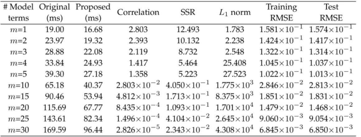
Table 1.Training times required and the corresponding results produced by the original and proposed approaches with varied small numbers of model terms (stable cases) in example 1
# Model terms Original (ms) Proposed (ms) Correlation SSR L1norm Training RMSE Test RMSE m=1 19.00 16.68 2.803 12.493 1.783 1.581×10⁻¹ 1.574×10⁻¹ m=2 23.97 19.32 2.393 10.132 2.238 1.424×10⁻¹ 1.417×10⁻¹ m=3 28.88 22.08 2.119 8.732 2.548 1.322×10⁻¹ 1.314×10⁻¹ m=4 33.84 24.93 1.417 5.464 25.408 1.045×10⁻¹ 1.037×10⁻¹ m=5 39.30 27.18 1.358 5.223 27.523 1.022×10⁻¹ 1.013×10⁻¹ m=10 65.18 40.37 2.803×10⁻² 4.050×10⁻¹ 1.775×10³ 2.846×10⁻² 2.813×10⁻² m=15 90.46 53.94 4.812×10⁻³ 1.713×10⁻¹ 8.375×10³ 1.851×10⁻² 1.831×10⁻² m=20 115.69 67.77 8.435×10⁻⁴ 1.093×10⁻¹ 1.701×10⁴ 1.479×10⁻² 1.468×10⁻² m=25 143.61 82.34 1.496×10⁻⁴ 4.104×10⁻² 2.645×10⁴ 9.060×10⁻³ 9.054×10⁻³ m=30 169.59 96.44 2.826×10⁻⁵ 2.343×10⁻² 4.308×10⁴ 6.845×10⁻³ 6.850×10⁻³
The Gaussian widthσwas assigned to a value of 0.7 to construct the candidate pool in which a total of 500 candidate model terms were produced at the beginning by taking all the training instances as the centres of potential basis functions. Both the original approach and our approach were used to perform the model selection, the process of selecting the first 30 model terms being shown in Table1. Here, the original approach was realised as in [53], in which the forward and backward substitutions were adopted to successively update the Cholesky decomposition and model parameters. In Table1, the training time, correlation, SSR,L1norm of model coefficients and training and test errors are listed for varied numbers of selected model terms. The model training times given in this table and the following tables in the paper were all averaged from a total of 50 runs of the respective approaches. Amongst those selected model terms, both the original and our methods were able to find the same terms to be included in the LIP model, giving the same values of correlations, SSRs,L1norms of coefficients and model errors. The effectiveness of our method has thus been demonstrated. In addition, the computational efficiency of the proposed approach in comparison to the original approach can be demonstrated by comparing between the second and third columns of Table1. This superiority became more significant when more model terms were included in the constructed model.
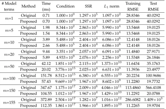
The selected model terms from the original approach and our approach started to differ from each other at step 45, with the corresponding training times, conditions of constructed regression matrices, SSRs,L1norms of coefficients and model errors, respectively, shown in Table
2. Due to standardisation, a number of model terms up toN−1(499 in this example) were successively included into the model in order to show the complete journey of the proposed algorithm and thus its efficiency. The condition number is seen generally increased during the model selection process as relatively more correlated terms are successively included into the model. Again, the computational efficiency of the proposed algorithm was always evident as in the third column of the table. The reason behind the differently selected model terms is mainly attributed to algorithm’s stability issues, owing to the gradually ill-conditioned regression matrix being constructed. In detail, as for the original algorithm, it is recognised that at every step the Cholesky decomposition performed on the explicit formulation of ΦTkΦk squares the system
15
Table 2.Training times required and the corresponding results produced by the original and proposed approaches with varied large numbers of model terms (unstable cases) in example 1
# Model terms Method Time (ms) Condition SSR L1norm Training RMSE Test RMSE m=10 Original 65.18 8.592×10 3 4.050×10⁻¹ 1.775×10³ 2.846×10⁻² 2.813×10⁻² Proposed 40.37 8.592×10³ 4.050×10⁻¹ 1.775×10³ 2.846×10⁻² 2.813×10⁻² m=45 Original 251.69 1.781×10 8 1.372×10⁻² 1.091×10⁶ 5.238×10⁻³ 5.220×10⁻³ Proposed 143.30 1.315×10⁸ 1.276×10⁻² 1.018×10⁶ 5.051×10⁻³ 5.025×10⁻³ m=50 Original 279.57 2.504×10 8 9.698×10⁻³ 2.358×10⁶ 4.404×10⁻³ 4.348×10⁻³ Proposed 159.00 2.926×10⁸ 1.166×10⁻² 9.156×10⁵ 4.828×10⁻³ 4.786×10⁻³ m=100 Original 612.80 8.325×10 11 1.432×10⁻² 2.473×10⁷ 5.352×10⁻³ 5.351×10⁻³ Proposed 338.50 2.261×10¹² 3.490×10⁻³ 8.950×10⁶ 2.642×10⁻³ 2.617×10⁻³ m=150 Original 1048.07 2.577×10 14 2.535×10⁻² 3.798×10⁷ 7.121×10⁻³ 7.006×10⁻³ Proposed 550.04 5.742×10¹³ 3.230×10⁻³ 1.279×10⁷ 2.542×10⁻³ 2.507×10⁻³ m=200 Original 1627.27 3.845×10 15 5.322×10⁻² 5.792×10⁷ 1.032×10⁻² 9.981×10⁻³ Proposed 756.15 1.208×10¹⁵ 2.926×10⁻³ 1.568×10⁷ 2.419×10⁻³ 2.392×10⁻³ m=250 Original 2341.37 2.096×10 16 1.284×10⁻¹ 9.070×10⁷ 1.602×10⁻² 1.530×10⁻² Proposed 1024.23 6.212×10¹⁵ 2.493×10⁻³ 1.477×10⁷ 2.233×10⁻³ 2.195×10⁻³ m=300 Original 3329.18 4.970×10 16 2.783×10⁻¹ 1.328×10⁸ 2.359×10⁻² 2.238×10⁻² Proposed 1256.22 4.443×10¹⁶ 2.404×10⁻³ 1.274×10⁷ 2.193×10⁻³ 2.167×10⁻³ m=350 Original 4570.16 9.080×10 16 7.439×10⁻¹ 2.148×10⁸ 3.857×10⁻² 3.639×10⁻² Proposed 1507.29 7.294×10¹⁶ 2.432×10⁻³ 1.199×10⁷ 2.205×10⁻³ 2.186×10⁻³ m=400 Original 6056.50 1.550×10 17 2.067×100 3.549×10⁸ 6.430×10⁻² 6.047×10⁻² Proposed 1679.56 1.563×10¹⁷ 2.399×10⁻³ 1.316×10⁷ 2.190×10⁻³ 2.166×10⁻³ m=450 Original 7862.22 3.568×10 17 2.388×101 1.192×10⁹ 2.185×10⁻¹ 2.049×10⁻¹ Proposed 1916.53 3.391×10¹⁷ 2.370×10⁻³ 1.388×10⁷ 2.177×10⁻³ 2.150×10⁻³ m=499 Original 9902.52 1.709×10 19 7.235×10⁴ 6.527×10¹⁰ 1.203×101 1.127×101 Proposed 2087.01 1.185×10¹⁹ 2.497×10⁻³ 3.118×10⁷ 2.235×10⁻³ 2.206×10⁻³ * It is noted that the proposed approach and the original approach started to choose different
model terms from model size 45 due to gradually ill-conditioned, selected regression matrices (causing potential instability issues).
condition number (i.e.,κ2(ΦTkΦk) =κ22(Φk)), where square roots are also engaged. In contrast,
our method is essentially derived from the orthogonalisation ofΦk(wherein this does not alter
the condition number, i.e.,κ2(Φk)). The corresponding orthogonal matrix is implicitly given by
Qk= [q1, . . . ,qk], whereqi=Ri−1pi/||Ri−1pi||2(i= 1, . . . , k). An upper triangular matrixAk)
is thereby resulted for solving the system only in the end of the model selection, plus avoiding square root operations as seen from updating all the scalars, matrices and vectors based on (3.8), i.e.,ρk+1,ck),γk,Ak),bk),dk)andΘˆm, according to (3.3)-(3.5), (3.16)-(3.18) and (3.23
)-(3.24). Consequently, the amplified condition number in the original algorithm means that the system being solved is more ill-conditioned (i.e., more sensitive to perturbations). In addition, in the original algorithm, when the selected model terms are not much correlated (i.e., matrix ΦTkΦk is positive-definite) as usually exhibited in the early stages of the model selection, the
numbers under the square roots are always positive. However, with the model size increases model terms with significant correlation are then inevitably selected, resulting in increasingly ill-conditioned matrix (aka near-singular matrix). In this case, the numbers under the square roots can be negative due to roundoff and accumulated errors, causing further instability issues for the original algorithm.
16 From the obtained SSR andL1norm of coefficients for those constructed models with different
sizes, it can also be seen that our method was more stable when encountered with ill-conditioned scenarios. In general, especially in the early stages of model selection, the SSR generated decreases as the model size increases. However, due to the increasing ill-conditioning of the constructed regression matrix thus causing instability issues, the SSR can then become larger when a large number of terms are included into the model. This can be seen from the results obtained by the original algorithm, confronting the large SSR increment since from a model size of 50 terms to 100 terms and thereafter. With the use of our algorithm, this instability issue caused by ill-conditioning is dramatically mitigated, where only slight increase in SSR can be seen when a large number of model terms are selected. For example, by comparing the SSR andL1norm produced by the original algorithm at steps 150 and 200, the instability issues apparently appeared where both SSR and L1 norm increased dramatically (from 2.535×10⁻² to 5.322×10⁻², and from 3.798×10⁷ to 5.792×10⁷, respectively). In contrast, our method produced much better results for these two values (decreased from 3.230×10⁻³to 2.926×10⁻³ for SSR, and increased from 1.279×10⁷ to 1.568×10⁷ for L1 norm). The situation became extremely worse for the original approach when more model terms were to be included in the final model as shown in the bottom part of Table 2, whereas this was considerably well for our approach. The numerical stability of our algorithm in comparison with the original approach was also reflected in the resultant training and test RMSEs (root mean squared errors) as shown in the last two columns of Table
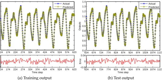
2. To retrieve a moderate size model and also prevent it from being seriously over-fitted and ill-conditioned, by adopting the AIC method as derived in (3.25)-(3.27), a total of 25 model terms can be selected to construct the LIP model for this example. Fig.1depicts the actual and predicted outputs of the system over the training and test datasets, showing a good representation of the chaotic behaviours for the model developed. The resultant training and test RMSEs are thereby 9.060×10⁻³and 9.054×10⁻³, respectively. 124 174 224 274 324 374 424 474 524 574 623 0.4 0.5 0.6 0.7 0.8 0.9 1 1.1 1.2 1.3 1.4 Outputs 124 174 224 274 324 374 424 474 524 574 623 −0.04 0 0.04 Time step Error Actual Predicted
(a) Training output
624 674 724 774 824 874 924 974 1024 1074 1123 0.4 0.5 0.6 0.7 0.8 0.9 1 1.1 1.2 1.3 1.4 Outputs 624 674 724 774 824 874 924 974 1024 1074 1123 −0.04 0 0.04 Time step Error Actual Predicted (b) Test output
Figure 1.The training and test outputs in chaotic time-series prediction (In each figure, the upper subfigure depicts the actual and predicted outputs, while the bottom subfigure shows the error between them).
(b) Number of sunspots forecasting
The number of sunspots being used to indicate the abundance of sunspots on the Sun, is recognised exhibiting nonlinear, non-stationary and non-Gaussian behaviours [54]. In this example, the yearly mean total number of sunspots from year 1700 to 2014 was adopted from WDC-SILSO (World Data Center - Sunspot Index and Long-term Solar Observations) [50]. The proposed method was thus applied to develop a LIP model to forecast the number of sunspots.
17 As in previous studies [54], the input vector for the model were defined asx(t) = [y(t−3), y(t−
2), y(t−1)], wheretdenotes the year index, and the output was to forecasty(t)of the sunspot number at yeart. The sunspot numbers for the first 156 years (i.e.,1703≤t≤1858) were used for training, with the trained model then applied to forecast the number of sunspots for the remaining 156 years (i.e.,1859≤t≤2014).
Table 3.Training times required and the corresponding results produced by the original and proposed approaches with varied numbers of model terms in example 2
# Model terms Method Time (ms) Condition SSR L1norm Training RMSE Test RMSE m=1 Original 0.71 1.000×10 0 1.297×10⁵ 1.097×10² 28.8346 40.0292 Proposed 0.70 1.000×100 1.297×10⁵ 1.097×10² 28.8346 40.0292 m=5 Original 1.98 8.344×10 2 2.863×10⁴ 5.990×10⁴ 13.5468 19.0125 Proposed 1.54 8.344×10² 2.863×10⁴ 5.990×10⁴ 13.5468 19.0125 m=10 Original 3.89 5.488×10 5 2.404×10⁴ 6.086×10⁶ 12.4148 18.0126 Proposed 2.66 5.488×10⁵ 2.404×10⁴ 6.086×10⁶ 12.4148 18.0126 m=20 Original 9.44 3.351×10 9 2.057×10⁴ 6.091×10⁹ 11.4840 27.9171 Proposed 5.89 4.933×10⁹ 2.076×10⁴ 2.256×10⁹ 11.5348 26.1846 m=50 Original 42.12 1.851×10 15 2.115×10⁴ 1.373×10¹⁰ 11.6434 35.1763 Proposed 20.02 3.776×10¹⁵ 2.025×10⁴ 6.631×10⁹ 11.3936 23.4977 m=100 Original 151.78 8.512×10 15 6.380×10⁴ 6.555×10¹⁰ 20.2234 100.9686 Proposed 57.43 9.669×10¹⁵ 1.967×10⁴ 8.602×10⁹ 11.2280 19.7732 m=150 Original 347.67 1.175×10 17 2.009×10⁶ 4.046×10¹¹ 113.4860 566.4108 Proposed 104.55 1.012×10¹⁷ 1.967×10⁴ 1.429×10¹⁰ 11.2292 20.0788 m=155 Original 372.89 2.504×10 17 1.282×10⁷ 1.016×10¹² 286.6082 1.409×10³ Proposed 112.35 1.861×10¹⁷ 1.966×10⁴ 1.895×10¹⁰ 11.2265 19.9704 * It is noted that the proposed approach and the original approach started to choose
different model terms from model size 20 due to gradually ill-conditioned, selected regression matrices (causing potential instability issues).
As in example 1, the Gaussian widthσ was assigned to 600 in this example and a total of 156 candidate model terms were generated. The training times, conditions of selected regression matrices, SSRs,L1norms and model errors under a varied number of selected model terms are listed in Table3for both the original and proposed approaches. It can be found that the training times consumed by our method were less than those consumed by the original approach, and this superiority was seen more significant as the number of included model terms increased. Meanwhile, our algorithm was able to perform same results as in the original approach when a number of up to 20 model terms were selected.
Due to ill-conditioning issues, it was found that, in comparison with the original approach, the proposed algorithm started to choose differing model terms since model size of 20. As the number of model terms as well as the condition of selected regression matrix increased, the proposed approach showed dramatic numerical stability than the original approach. When a total of 155 model terms were selected, the SSRs resulting from the proposed and original approaches were 1.966×10⁴and 1.282×10⁷, respectively, while the correspondingL1norms were 1.895×10¹⁰and 1.016×10¹², respectively. Correspondingly, the training and test RMSEs from our algorithm were also found to be much better than from the original approach. For the original approach, due to instability issues, the model errors continued to increase after a certain number of model terms have been included in the model. The overfitting issues, however, can somewhat be observed from this example, although it is not obvious for our method. A subset of five model terms can be
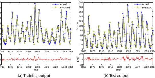
18 adopted by using the AIC method, the results being depicted in Fig.2. The corresponding RMSEs
on the training and test dataset were 13.5468 and 19.0125, respectively.
1703 1723 1743 1763 1783 1803 1823 1843 1858 −20 0 20 40 60 80 100 120 140 160 Outputs 1703 1723 1743 1763 1783 1803 1823 1843 1858 −100 0 100 Year Error Actual Predicted
(a) Training output
18590 1879 1899 1919 1939 1959 1979 1999 2014 20 40 60 80 100 120 140 160 180 200 Outputs 1859 1879 1899 1919 1939 1959 1979 1999 2014 −100 0 100 Year Error Actual Predicted (b) Test output
Figure 2.The training and test outputs in forecasting the number of sunspots (In each figure, the upper subfigure depicts the actual and predicted outputs, while the bottom subfigure shows the error between them).
(c) Australian credit approval
In this example, the Statlog dataset consisting of the information of Australian credit card applications obtained from the UCI machine learning repository [51] is considered. For privacy protection, the names and values of attributes for the dataset were initially altered to be physically meaningless, where a total of 14 input attributes are included. The output attribute is used to indicate either the approval or the refusal of a credit card application. There are 690 instances in the dataset, from which 37 instances involve missing values (replaced with artificially computed values). The whole dataset was then randomly and equally partitioned into a training and a test dataset for this study.
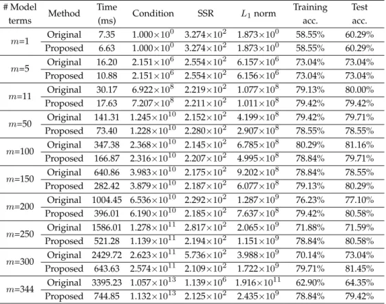
The Gaussian widthσwas chosen as 5.0×10⁷and a total of 345 candidate model terms were obtained. As in examples 1 and 2, the training times, conditions of selected regression matrices, SSRs,L1norms and model accuracies for various subsets of selected model terms for both the original and proposed approaches are given in Table4. The superiority of our approach in terms of consuming less training time and providing more stable results was once again confirmed. In this example, differing model terms started to be chosen since step 11 from the two approaches, resulting in a remarkable difference between them when a total of 344 model terms were included into the model (SSR: 2.125×10²and 1.139×10⁶;L
1norm: 2.435×10⁹and 1.916×10¹¹). After a few model terms that have been selected, the test accuracy has stabilised around 80% for our approach while this is not the case for the original approach. A total of six model terms can be chosen to construct the final classifier for this example by using the AIC method, giving the training and test accuracies of 77.97% and 80.58%, respectively.
5. Conclusion
An efficient least angle regression algorithm was proposed in this paper for the construction of a class of LIP (linear-in-the-parameters) models. The algorithm proceeds in a stepwise manner, each step adding a new model term into the LIP model, with the effect of minimising model residuals andL1 norm of coefficients. It is a less greedy model selection method and proceeds
19
Table 4.Training times required and the corresponding results produced by the original and proposed approaches with varied numbers of model terms in Example 3
# Model terms Method Time (ms) Condition SSR L1norm Training acc. Test acc. m=1 Original 7.35 1.000×10 0 3.274×10² 1.873×100 58.55% 60.29% Proposed 6.63 1.000×100 3.274×10² 1.873×100 58.55% 60.29% m=5 Original 16.20 2.151×10 6 2.554×10² 6.157×10⁶ 73.04% 73.04% Proposed 10.88 2.151×10⁶ 2.554×10² 6.156×10⁶ 73.04% 73.04% m=11 Original 30.17 6.922×10 8 2.219×10² 1.077×10⁸ 79.13% 80.00% Proposed 17.63 7.207×10⁸ 2.211×10² 1.011×10⁸ 79.42% 79.42% m=50 Original 141.31 1.245×10 10 2.152×10² 4.199×10⁸ 79.42% 79.71% Proposed 73.40 1.228×10¹⁰ 2.280×10² 2.907×10⁸ 78.55% 78.55% m=100 Original 347.38 2.368×10 10 2.145×10² 6.785×10⁸ 80.29% 81.16% Proposed 166.87 2.316×10¹⁰ 2.207×10² 4.995×10⁸ 78.84% 79.71% m=150 Original 640.86 3.983×10 10 2.175×10² 9.202×10⁸ 78.84% 78.55% Proposed 282.42 3.879×10¹⁰ 2.187×10² 6.077×10⁸ 79.13% 80.29% m=200 Original 1004.45 6.536×10 10 2.292×10² 1.287×10⁹ 76.23% 77.10% Proposed 396.01 6.190×10¹⁰ 2.185×10² 7.637×10⁸ 79.42% 80.58% m=250 Original 1586.01 1.278×10 11 2.817×10² 2.065×10⁹ 71.88% 71.59% Proposed 521.28 1.139×10¹¹ 2.194×10² 1.151×10⁹ 78.84% 80.58% m=300 Original 2429.72 2.623×10 11 5.736×10² 3.988×10⁹ 70.14% 73.04% Proposed 643.63 2.574×10¹¹ 2.109×10² 1.722×10⁹ 79.71% 81.45% m=344 Original 3395.23 1.057×10 13 1.139×10⁶ 1.916×10¹¹ 62.90% 64.35% Proposed 744.85 1.132×10¹³ 2.125×10² 2.435×10⁹ 78.84% 79.42% * It is noted that the proposed approach and the original approach started to choose different
model terms from model size 11 due to gradually ill-conditioned, selected regression matrices (causing potential instability issues).
equiangularly between all the selected model terms by means of their resultant correlations with model errors at every subset selection step. Unlike the original approach where the well-known Cholesky decomposition was employed, an efficient recursive algorithm was proposed to solve the least angle regression without the need of matrix inversions, decompositions and transformations. The correlations between model terms and residuals, the evolving directions, together with other pertinent variables, were explicitly formulated and are recursively updated in the proposed algorithm. The model coefficients are only computed when the algorithm finishes. The computational complexity of the proposed approach was also well analysed and confirmed to be more efficient than the original approach. Finally, three artificial and real-world illustrative examples were used to demonstrate the effectiveness and efficiency of the proposed algorithm, where its numerical stability was also found to be another strength. As mentioned previously, given the connection between LAR and Lasso, future research includes deriving the efficient algorithm for retrieving Lasso solutions for performing tasks such as model or variable selection. On the other hand, the integration of hyperparameter learning for enhanced model performance is another direction of research.
Ethics. This research does not contain human or animal subject.
Data Accessibility. All the experimental data are accessible from the references cited in the correponding examples in the paper.
20
Authors’ Contributions. W.Z. developed the algorithm, conducted the simulation and drafted the manuscript. T.H.B. and Y.R. coordinated the research, helped to interpret the results and revised the manuscript. All authors gave final approval for publication.
Competing Interests. We have no competing interests.
Funding. The work was supported by the EU Seventh Framework Programme (FP7) under Grant 619795.
Acknowledgements. The authors acknowledge the editors and reviewers for their constructive comments and suggestions for improving the quality of this paper.
References
1. Hong X, Harris CJ, Chen S, Sharkey PM. 2003 Robust nonlinear model identification methods using forward regression.IEEE Trans. Syst., Man, Cybern. A, Syst. Hum.33, 514–523. (doi:10. 1109/TSMCA.2003.809217)
2. Billings SA, Wei HL. 2007 Sparse model identification using a forward orthogonal regression algorithm aided by mutual information.IEEE Trans. Neural Netw.18, 306–310. (doi:10.1109/ TNN.2006.886356)
3. Li K, Peng JX, Irwin GW. 2005 A fast nonlinear model identification method.IEEE Trans. Autom. Control50, 1211–1216. (doi:10.1109/TAC.2005.852557)
4. Han HG, Qiao JF. 2012 Adaptive computation algorithm for RBF neural network.IEEE Trans. Neural Netw. Learn. Syst.23, 342–347. (doi:10.1109/TNNLS.2011.2178559)
5. Wang L, Truong DN. 2013 Stability enhancement of a power system with a PMSG-based and a DFIG-based offshore wind farm using a SVC with an adaptive-network-based fuzzy inference system.IEEE Trans. Ind. Electron.60, 2799–2807. (doi:10.1109/TIE.2012.2218557) 6. Wu X, Ró ˙zycki P, Wilamowski BM. 2015 A hybrid constructive algorithm for single-layer
feedforward networks learning.IEEE Trans. Neural Netw. Learn. Syst.26, 1659–1668. (doi:10. 1109/TNNLS.2014.2350957)
7. Billings SA, Chen S, Korenberg MJ. 1989 Identification of MIMO non-linear systems using a forward-regression orthogonal estimator.Int. J. Control49, 2157–2189. (doi:10.1080/ 00207178908961377)
8. Aguirre LA. 1997 On the structure of nonlinear polynomial models: higher order correlation functions, spectra, and term clusters.IEEE Trans. Circuits Syst. I, Fundamental Theory Appl.44, 450–453. (doi:10.1109/81.572342)
9. Pukish MS, Ró ˙zycki P, Wilamowski BM. 2015 Polynet: A polynomial-based learning machine for universal approximation.IEEE Trans. Ind. Inf.11, 708–716. (doi:10.1109/TII.2015.2426012) 10. Er MJ, Wu S, Lu J, Toh HL. 2002 Face recognition with radial basis function (RBF) neural
networks.IEEE Trans. Neural Netw.13, 697–710. (doi:10.1109/TNN.2002.1000134)
11. Chen H, Gong Y, Hong X. 2013 Online modeling with tunable RBF network.IEEE Trans. Cybern.43, 935–947. (doi:10.1109/TSMCB.2012.2218804)
12. Yu H, Reiner PD, Xie T, Bartczak T, Wilamowski BM. 2014 An incremental design of radial basis function networks.IEEE Trans. Neural Netw. Learn. Syst.25, 1793–1803. (doi:10.1109/ TNNLS.2013.2295813)
13. Chiang JH, Hao PY. 2004 Support vector learning mechanism for fuzzy rule-based modeling: A new approach.IEEE Trans. Fuzzy Syst.12, 1–12. (doi:10.1109/TFUZZ.2003.817839) 14. Juang CF, Hung CW, Hsu CH. 2014 Rule-based cooperative continuous ant colony
optimization to improve the accuracy of fuzzy system design.IEEE Trans. Fuzzy Syst.22, 723–735. (doi:10.1109/TFUZZ.2013.2272480)
15. Zhao W, Zhang J, Li K. 2015 An efficient LS-SVM-based method for fuzzy system construction.IEEE Trans. Fuzzy Syst.23, 627–643. (doi:10.1109/TFUZZ.2014.2321594) 16. Zhang Y, Liu Y. 2009 Data imputation using least squares support vector machines in urban
arterial streets.IEEE Signal Process. Lett.16, 414–417. (doi:10.1109/LSP.2009.2016451) 17. Yu L, Chen H, Wang S, Lai KK. 2009 Evolving least squares support vector machines for stock
market trend mining.IEEE Trans. Evol. Comput.13, 87–102. (doi:10.1109/TEVC.2008.928176) 18. Zhang J, Li K, Irwin GW, Zhao W. 2012 A regression approach to LS-SVM and sparse realization based on fast subset selection. inProc. 10th Word Congr. Intell. Control Autom. Beijing 612–617 (doi:10.1109/WCICA.2012.6357952)