SMALL SAMPLE MULTIPLE TESTING
WITH APPLICATION TO CDNA MICROARRAY DATA
A Dissertation by
ERIC POOLE HINTZE
Submitted to the Office of Graduate Studies of Texas A&M University
in partial fulfillment of the requirements for the degree of DOCTOR OF PHILOSOPHY
August 2005
SMALL SAMPLE MULTIPLE TESTING
WITH APPLICATION TO CDNA MICROARRAY DATA
A Dissertation by
ERIC POOLE HINTZE
Submitted to the Office of Graduate Studies of Texas A&M University
in partial fulfillment of the requirements for the degree of DOCTOR OF PHILOSOPHY
Approved by:
Chair of Committee, Michael Sherman Committee Members, F. Michael Speed Marina Vannucci Rajesh C. Miranda Head of Department, Simon Sheather
August 2005 Major Subject: Statistics
ABSTRACT
Small Sample Multiple Testing with Application to cDNA Microarray Data. (August 2005) Eric Poole Hintze, B.S., Brigham Young University;
M.S., Brigham Young University
Chair of Advisory Committee: Dr. Michael Sherman
Many tests have been developed for comparing means in a two-sample scenario. Microarray experiments lead to thousands of such comparisons in a single study. Several multiple testing procedures are available to control experiment-wise error or the false discovery rate. In this dissertation, individual two-sample tests are compared based on accuracy, correctness, and power. Four multiple testing procedures are compared via simulation, based on data from the lab of Dr. Rajesh Miranda. The effect of sample size on power is also carefully examined. The two sample t-test followed by the Benjamini and Hochberg (1995) false discovery rate controlling procedure result in the highest power.
ACKNOWLEDGMENTS
I thank my advisor, Dr. Michael Sherman, for his positive advice throughout the development of the dissertation. I thank Dr. F. Michael Speed for his encouragement and help with computational resources. I thank Dr. Marina Vannucci and Dr. Rajesh Miranda for their help in the understanding of microarrays. I also thank Dr. Miranda for allowing me to use his data in the dissertation.
I especially thank my wife, Valora, for her constant support, love, and patience. I thank my children, Spencer, Ashley Jo, and Brooklyn, for making my dissertation experience a complete adventure.
TABLE OF CONTENTS
Page
ABSTRACT………. iii
ACKNOWLEDGMENTS……… iv
TABLE OF CONTENTS………. v
LIST OF FIGURES……….. vii
LIST OF TABLES……… ix
1. INTRODUCTION………..………. 1
2. TWO SAMPLE TESTS……… 4
2.1. Background………. 4
2.2. General Comparison of the t-test, Welch’s t-test, the Bootstrap Within Test, the Bootstrap Across Test, and the Permutation Test……… 9
2.2.1. Permutation Achieved Significance Levels………. 10
2.2.2. Bootstrap Achieved Significance Levels………. 11
2.2.3. Comparison of Null Distributions………... 12
2.2.4. Accuracy and Correctness……… 13
2.2.4.1. Definitions and ASL Formulation………. 13
2.2.4.2. Estimated Test Size Comparison……….….. 14
2.2.4.3. Two Sample Test Accuracy Comparison………….. 15
2.2.4.4. Power………. 15
2.2.4.5 Comparison of Correctness……….... 16
2.3. Two Sample Test Discussion and Recommendations………. 20
3. MULTIPLE TESTING ADJUSTMENT……….………. 23
3.1. Historical Perspective……….. 23
3.2. Present Microarray Multiple Testing Problem………. 27
3.3. Details of Adjustment Methods Compared………. 30
3.3.1. Bonferroni Adjustment………. 30
3.3.2. Benjamini and Hochberg’s (1995) False Discovery Rate Control Procedure………. 30
3.3.3. Westfall and Young’s (1993) Single Step maxT Resampling Based Procedure……….... 31
3.3.4. Efron’s (2004) Empirical Null Distribution Local False Discovery Rate Method………... 32
Page
4. MICROARRAY DATA DETAILS………..………. 36
4.1. Data Normalization in Microarrays………. 36
4.2. Miranda Data Summary………... 38
4.2.1. Distribution Shape………. 38
4.2.2. Variance………. 40
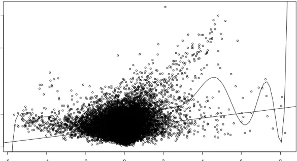
4.2.3. Mean – Standard Deviation Relationship……….. 40
4.2.4. Miranda Data Results ……….……….. 41
5. SIMULATION STUDY………..………….. 44
5.1. Setup……… 44
5.1.1. Number of Genes……….. 44
5.1.2. Proportion of Differentially Expressed Genes……….. 44
5.1.3. Magnitude of Differential Expression………... 44
5.1.4. Testing Methods………... 45
5.1.5. Sample Size………... 46
5.1.6. Test Level……….. 47
5.1.7. Number of Simulations………. 47
5.1.8. Error Rates……… 47
5.1.9. Correlation Among Genes……… 47
5.2. Results………. 48
5.3. Summary and Discussion.………... 50
6. CONCLUSIONS………..………. 55 REFERENCES………... 57 APPENDIX A……… 64 APPENDIX B……… 84 APPENDIX C……… 100 APPENDIX D……… 109 APPENDIX E……… 116 APPENDIX F……… 118 APPENDIX G……… 240 VITA……….. 272
LIST OF FIGURES
FIGURE Page
1 First in a Series of Four Figures Depicting the Variation in Area Outside 2.306 When 4 Different
Tests Are Used, t-distribution……….. 18
2 Second in a Series of Four Figures Depicting the Variation in Area Outside 2.306 When 4 Different Tests Are Used, Permutation Distribution.……….. 18
3 Third in a Series of Four Figures Depicting the Variation in Area Outside 2.306 When 4 Different Tests Are Used, Bootstrap Within t Distribution………. 19
4 Fourth in a Series of Four Figures Depicting the Variation in Area Outside 2.306 When 4 Different Tests Are Used, Bootstrap Across t Distribution.……… 19
5 Empirical Distribution Estimation.………... 34
6 Plot of f z( ) and f z0( ) for All of the 10,000 Simulated z-values ……… 35
7 Histogram of 133,656 Standardized Residuals from Miranda Data………..………. 39
8 Histogram of 133,656 Standardized Residuals from Standard Normal Simulated Data……… 39
9 Histogram of Variances from Expression Data for All 22,276 Genes….………. 40
10 Scatter Plot of Standard Deviation vs. Mean for 22,276 Genes………. 41
11 Histogram of 22,276 z-values from Mianda Expression Data...……….…… 42
12 Distribution of Magnitudes of Difference for Simulated Differentially Expressed Genes...……… 45
13 Power Curve for 200 Gene Scenarios……...……… 51
14 Power Curve for 2,000 Gene Scenarios……...………. 52
FIGURE Page 16 Power Curve for 2,000 Gene Scenarios with
LIST OF TABLES
TABLE Page
1 Number of Possible Unique Resampling Statistics from Three Resampling Methods for the Two Sample
Test Scenario……… 22
2 Benjamini and Hochberg’s (1995) Table Used to Define the False Discovery Rate ..……….. 28
3 Smallest 10 Raw, Bonferroni, and Benjamini and Hochberg False Discovery Rate Adjusted P-values for the Miranda Study………...……….. 42
4 Smallest 10 Local False Discovery Rates for Miranda Data Using Efron’s Method….. ..……….. 43
5 Simulation Testing Procedures and Titles……… 46
6 Summary of Figures of Appendix F..………..………. 48
1. INTRODUCTION
A common problem in genomics is determining which among the thousands of genes in the DNA of an organism are differentially expressed when a treatment is given. Until recently, the number of genes in humans was commonly cited to be around 100,000. The human genome projects of Celera and the public consortium of scientists both found the number of genes in humans instead to be around 40,000, “give or take a few thousand” (Pennisi, 2001). Forty-thousand might still be considered a formidable number of genes to examine were it not for developments in DNA and RNA technology. These developments allow scientists to gather expression data about thousands of genes at a time using microarrays.
On a microarray there are several thousand probes of known identity, each corresponding to a gene of interest. The mRNA expressed in an individual is obtained from some of the individual’s cells (i.e., blood or tissue) and converted to fluorescently labeled cDNA. When the cDNA is exposed to a microarray, its segments bind preferentially to the probes to which they complement. The cDNA corresponding to the mRNA from genes which are expressed in higher quantities will hybridize to the corresponding probe in higher quantities. The amount of hybridized material for each probe can then be measured using the intensity of fluorescence from each probe when exposed to laser scanning. The result is several thousand intensities that correspond in some degree to the amount of mRNA expression for each of those genes in that individual. This can be repeated among several individuals who have and have not received a treatment of interest.
By comparing the intensities of expression of control individuals and treatment individuals, specific genes which are differentially expressed may be determined using a statistical test. Due to the variation in gene expression from individual to individual and the sheer number of comparisons, it is clear that if genes are compared without
_____________
adjustment for multiplicity, some (or many) will be declared different by chance alone. It is desirable for researchers to limit the number of genes which are wrongly declared to be differentially expressed, but at the same time find as many of the genes as possible for which expression truly is different.
Superior methods for determining which genes are to be declared differentially expressed should be successful in two ways. First, the method should do well at assigning low individual unadjusted P-values to genes which are expressed differently in the control and treatment groups. Conversely, high P-values should be assigned to those genes which are not differentially expressed. Second, the method should make efficient use of the individual P-values so as to identify the most differentially expressed genes while appropriately limiting the number of false positives.
One distinguishing feature of microarray experiments is sample size. Although the price of producing microarray data has steadily decreased, the number of replicates in a microarray experiment is typically in the range of 2 to 5 (Yang and Speed, 2003).
Another common feature in microarray experiments is dependent gene expression. There are many groups of genes which are co-regulated and thus have correlated (sometimes highly) expression levels. This casts doubt on the assumption of independence of tests.
The purpose of this dissertation is two-fold. First, I compare several common two-sample testing methods under several distributional conditions in terms of accuracy
and correctness, which are defined in the text. The focus is determining the proper test
for comparing microarray expression levels with small sample sizes (e.g., n = 3 or 5). The primary methods compared are the t-test (Fisher, 1925), Welch’s (1947, 1949) t-test, the permutation test, and two bootstrap t-tests. I discuss briefly some other nonparametric tests such as the two sample median test, Fisher’s (1934) exact test, the Wilcoxon (1945) rank test (also called Wilcoxon signed rank test or Wilcoxon-Mann-Whitney test [Mann and Wilcoxon-Mann-Whitney, 1947]), and the use of trimmed means.
The second major objective of the dissertation is determining how the accuracy and correctness of the individual tests affect the identification of differentially expressed
genes when thousands of comparisons are made simultaneously. These are measured in terms of family-wise error rate, false discovery rate, and power. Multiple testing adjustment procedures compared will be the Bonferroni correction procedure, Benjamini and Hochberg’s (1995) false discovery rate control procedure, and Westfall and Young’s (1993) single step maxT resampling based procedure. I also explore the construction of the empirical null hypothesis, recently described by Efron (2004).
Comparisons of these methods are made via simulation and microarray data provided by the lab of Dr. Rajesh Miranda (Texas A&M University, Departments of Anatomy and Neurobiology). An experiment was run in the Miranda lab to examine the effect of CD133 on gene expression. It is of interest to determine which among 22,276 genes are up- or down-regulated when cells are injected with CD133, which is known to cause cells to differentiate. Three experimental units received the CD133 treatment and 3 were controls. Microarray measurements of expression intensity were made for each of the 22,276 genes for the 6 experimental units.
The details of the two sample tests, multiple testing adjustment procedures, microarray data normalization, and simulations are described in the sections that follow.
2. TWO SAMPLE TESTS 2.1. Background
The problem of comparing two population means has been studied extensively over the past hundred years. The null hypothesis is that the means are equal,
2 1
0 :μ =μ
H ,
with three common alternative hypotheses,
2 1 :μ <μ a H , Ha :μ1 ≠μ2, or 2 1 :μ >μ a H ,
which are selected according to the nature of the experiment or study. The most common test statistic used for evaluation of the chosen hypotheses based on samples
1 1 11, ,yn y K and 2 2 21, ,y n y K is the t-statistic 2 1 2 1 1 1 n n s y y t + − = , with 2 ) 1 ( ) 1 ( 2 1 2 2 2 2 1 1 2 − + − + − = n n s n s n
s , where s12and s22 are the usual sample variances. If samples 1 1 11, ,yn y K and 2 2 21, ,y n
y K come from two normal populations with equal variances then the statistic t is known to follow “Student’s” t distribution with degrees of freedom equal to n1 +n2 −2 (Fisher, 1925). An appropriate P-value for the test may then be calculated as the probability of t being as or more extreme than the one obtained, based on this distribution. Problems may arise, however, when the two underlying distributions are not normally distributed and/or have differing variances. These problems are often amplified when the sample sizes also differ. Unfortunately in practice little is usually known about the true underlying distributions from which the two samples come, particularly when sample sizes are small.
To understand the effect of nonnormality on t, consider two samples y1 and y2
from populations with mean zero and unit variance, but with (possibly) differing skewness, say γ1(y1)and γ1(y2), and/or (possibly) differing kurtosis, say γ2(y1)and
)
( 2
2 y
γ . The distribution of each of the two populations can be described nearly by the first four terms of the Edgeworth expansion:
) ( 72 ) ( ! 4 ) ( ! 3 ) ( ) ( (6) 2 1 ) 4 ( 2 ) 3 ( 1 x x x x x f =φ −γ φ +γ φ +γ φ
where φ(x) is the p.d.f. of the standard normal distribution and φ(r)(x)its rth derivative. Building upon the work of Geary (1947), Gayen (1950) used this expansion to derive the first four raw (not central) moments of t:
(
)
(
)(
)
⎪⎭ ⎪ ⎬ ⎫ ⎪⎩ ⎪ ⎨ ⎧ ⎟⎟ ⎠ ⎞ ⎜⎜ ⎝ ⎛ + − + + ⎟⎟ ⎠ ⎞ ⎜⎜ ⎝ ⎛ − − − ≅ ′ 2 2 2 2 1 1 2 2 1 1 1 2 2 2 2 1 1 1 2 1 1 1 4 3 1 2 ) ( ) ( 2 1 2 1 ) ( ) ( 2 1 1 ) ( v v n n n n y y v v y y v t γ γ γ γ μ ,(
)
(
)
⎪⎩ ⎪ ⎨ ⎧ − − + ⎟⎟ ⎠ ⎞ ⎜⎜ ⎝ ⎛ + + ≅ ′ 2 2 2 1 2 1 2 2 2 2 1 2 1 2 2 2 1 2 1 ) ( ) ( 6 2 1 1 ) ( v n n n n y y v v v v t γ γ μ(
) (
)
(
) (
2)
2 1 2 2 1 1 1 2 2 1 2 1 2 1 2 2 2 1 2 8 5 16 ) ( ) ( 1 2 ) ( ) ( v v y y v v n n n n y y ⎟⎟ + − − ⎠ ⎞ ⎜⎜ ⎝ ⎛ − − + + γ γ γ γ(
)(
)
(
)
⎭ ⎬ ⎫ + − − − + 2 2 1 2 2 2 1 1 3 2 2 1 2 1 2 2 2 2 1 1 2 1 8 5 ) ( ) ( 27 4 ) ( ) ( v v y y v n n n n y y γ γ γ γ ,(
)
(
)
⎪⎭ ⎪ ⎬ ⎫ ⎪⎩ ⎪ ⎨ ⎧ ⎟⎟ ⎠ ⎞ ⎜⎜ ⎝ ⎛ − + + ⎟⎟ ⎠ ⎞ ⎜⎜ ⎝ ⎛ − + − ≅ ′ 2 2 2 1 2 1 1 1 2 1 2 2 2 1 2 1 1 1 2 3 1 3 1 1 ) ( ) ( 2 1 9 1 1 ) ( ) ( 2 1 1 ) ( n n y y n n n n y y v t γ γ γ γ μ ,(
) (
2 1) (
2 1)
2 2 1 1 4 2 2 1 2 1 2 2 2 1 2 2 1 2 1 2 2 2 1 18 102 12 ( ) 3 ( ) ( ) 2 n n n n v v t v y y v v v n n n n v v μ′ ≅ ⎨⎜⎪⎧⎛ + + ⎟⎞ + γ −γ − ⎜⎛⎜ − ⎛⎜ − ⎞⎟ ⎝ ⎠ ⎝ ⎠ ⎪ ⎝ ⎩ 1 1 2 2 2 18v 66v v v ⎞ − − ⎟ ⎠(
) (
)
⎟ ⎟ ⎠ ⎞ ⎜ ⎜ ⎝ ⎛ ⎟⎟ ⎠ ⎞ ⎜⎜ ⎝ ⎛ − − ⎟⎟ ⎠ ⎞ ⎜⎜ ⎝ ⎛ − − + + 2 2 2 1 2 2 1 2 2 2 1 2 2 1 2 1 2 1 2 2 2 1 2 15 2 12 2 ) ( ) ( v v v v v v v v n n n n y y γ γ(
)
(
) (
)
⎟⎟ ⎠ ⎞ ⎜ ⎜ ⎝ ⎛ ⎟⎟ ⎠ ⎞ ⎜⎜ ⎝ ⎛ − − − + + + − − + 2 1 2 2 2 2 1 2 1 2 2 2 1 1 2 1 2 2 1 1 1 4 27 4 48 26 3 2 12 ) ( ) ( n n v n n n n v v v v v y y γ γ
(
)(
)
(
)
⎟⎟ ⎠ ⎞ ⎜ ⎜ ⎝ ⎛ ⎟⎟ ⎠ ⎞ ⎜⎜ ⎝ ⎛ + − + ⎟⎟ ⎠ ⎞ ⎜⎜ ⎝ ⎛ − − − + 2 2 2 2 2 2 1 2 1 2 2 2 1 2 1 2 1 2 2 2 1 2 2 1 1 2 1 1 2 1 27 81 4 ) ( ) ( v v n n n n v v v v n n n n y y γ γ(
)
(
)
⎪⎭ ⎪ ⎬ ⎫ ⎟ ⎟ ⎠ ⎞ ⎜ ⎜ ⎝ ⎛ − − + + 2 2 3 2 3 1 2 2 1 2 2 2 2 2 1 2 2 1 1 1 1 4 27 6 ) ( ) ( v n n n n v v y y γ γ .where n1 and n2 are the sample sizes and
2 1 1 1 1 n n v = + , v2 =n1+n2 −2
From these approximate moments, approximate central moments of t can be constructed using (see, e.g., Stuart and Ord, 1994)
2 1 2 2(t) μ (t) μ (t) μ = ′ − ′ , 3 1 1 2 3 3(t) μ (t) 3μ (t)μ (t) 2μ (t) μ = ′ − ′ ′ + ′ , 4 1 2 1 2 1 3 4 4(t) μ (t) 4μ (t)μ (t) 6μ (t)μ (t) 3μ (t) μ = ′ − ′ ′ + ′ ′ − ′ ,
which can then be used to calculate the approximate skewness and kurtosis of t using
3 3 2 3 2 3 1 ) ( E ) ( ) ( ) ( t t t t t t σ μ μ μ γ = = − , 3 ) ( E 3 ) ( ) ( ) ( 4 4 2 2 4 2 − − = − = t t t t t t σ μ μ μ γ .
The skewness and kurtosis of a true ‘Student’s’ t-distribution are
0 ) (
1 t =
γ , γ2(t)=6/(η−4), η>4
where η represents the degrees of freedom. Comparisons between the estimated and expected theoretical distributions can be made to determine the effects of nonnormality of the two sampled distributions on the distribution of the test statistic t. Alternatively, the distribution of t can be simulated.
In general, if n1 ≅n2and if one can assumeγ1(y1)≅γ1(y2) and γ2(y1)≅γ2(y2), then the skewness and kurtosis of the sampled distributions will have very little effect on the distribution of the t-statistic. Pearson and Please (1975) simulated 2,000 pairs of samples of equal sample size, skewness, and kurtosis of size 10 and 25 from
distributions ranging in skewness (γ1(y1)=γ1(y2)) from 0 to 0.8, and kurtosis
(γ2(y1)=γ2(y2)) from -1 to 1.4. Almost without exception the proportion of the 2,000
tests with t-statistics in the outer 5% of the tails was between 0.04 and 0.06. Similar results were found by Pearson (1929). When sample size, skewness, and kurtosis are not approximately equal, less is known of what the distribution of the t-statistic may be, mostly because of the enormity of the number of possible combinations of n1,n2,
) ( ),
( 1 1 2
1 y γ y
γ ,γ2( ),y1 and γ2(y2). A reasonable idea might be obtained by estimating these parameters and using Gayen’s approximate moments described above to get reasonable estimates of γ1(t) and γ2(t). Unfortunately, samples of size five or even ten do not allow for accurate estimation of skewness and kurtosis of underlying distributions. Some larger sample examples are given in Geary (1947) and Gayen (1950).
An oft-used technique for correcting for non-normality is the use of transformations such as the logarithmic or square root transformations. Transformations may be particularly useful if there appear to be marked differences in variances among the samples. A difficulty that arises in transforming two groups occurs when one group appears to benefit from a transformation while the other does not.
Nonparametric and/or robust estimation techniques are also often employed when the distributional assumptions of the common t-test are not met. The two sample median test, Fisher’s (1934) exact test, the Wilcoxon (1945) rank test (also called Wilcoxon signed rank test or Wilcoxon-Mann-Whitney test [Mann and Whitney, 1947]), Pitman’s (1937) permutation test, the bootstrap method (Efron, 1979, 1982), and the use of trimmed means are examples of such techniques, the Wilcoxon rank test being the most popular. For details, see, for example, Miller (1986), or Ostle and Malone (1988). These methods are often considered to be useful when outliers are present.
Recent simulation studies indicate that (at least) some non-parametric rank procedures (i.e., Wilcoxon’s sign rank test) perform very poorly when variance heterogeneity is a problem, even for equal sample sizes. The inferiority in performance is even more pronounced when the underlying distributions are skewed, which is the
usual reason for using such tests (see Zimmerman, 2004). Use of rank tests is not recommended when equality of variance is in question.
Differing variances among the two populations sampled can also be a formidable challenge in a two sample comparison, especially when the sample sizes differ. Miller (1986) notes that for the usual t-statistic, “the variance for the larger sample tends to dominate the denominator of the t-statistic.” Transformations can be useful in correcting the problem of unequal variance. Another approach is to use a different t-test. When the populations compared have unequal variance, but are both normally distributed, the resulting test of H0 :μ1 =μ2 is known as the Behrens-Fisher problem. The statistic usually recommended for testing in this scenario is one developed by Welch (1947, 1949). The statistic is 2 2 2 1 2 1 2 1 n s n s y y tW + − =
or Welch’s t-statistic. The use of this statistic relies on the asymptotic convergence of the sample variances to the true variances, and is certainly appropriate for large samples. For small or moderate samples tW approximates ‘Student’s’ t-distribution, with estimated degrees of freedom
2 2 2 2 2 2 1 2 1 1 2 2 2 2 1 2 1 1 1 1 1 ˆ ⎟⎟ ⎠ ⎞ ⎜⎜ ⎝ ⎛ − + ⎟⎟ ⎠ ⎞ ⎜⎜ ⎝ ⎛ − ⎟⎟ ⎠ ⎞ ⎜⎜ ⎝ ⎛ + = n s n n s n n s n s v .
The statistic tW usually outperforms t (higher power when nominal α is preserved) when
the variances of the sampled populations differ considerably (Welch, 1947, 1949). When
1 2
n =n , t and tW are equivalent, except for the degrees of freedom used in the test.
Using the first four terms of the Edgeworth series, Bhattacharjee (1968) derived the approximate distribution of t and tW based on n1,n2, γ1(y1),γ1(y2), γ2( ),y1 γ2(y2), and σ1 and σ2, thus generalizing the work of Geary (1947) and Gayen (1950) to allow
for unequal variances. Bhattacharjee’s illustrations show a wide range of effects of various combinations of these parameters on the two-sided tail area of t and tW as
compared to the customary ‘Student’s’ t distribution two-sided tail area. It should be noted that Bhattacharjee uses degrees of freedom n1 +n2 −2 for both t and tW, and not adjusted degrees of freedom for tW. Bhattacharjee concludes “If the populations are non-normal and the variances are unequal, the non-normal theory tests on the basis of the criteria [t and tW], may under certain circumstances give misleading results. The effect may,
however, be minimized by taking samples with equal number of observations.”
In the context of microarray data, the sample sizes are usually very small. The chips used for a microarray experiment are currently very expensive so that only a small number (perhaps 2-5) of individuals are typically in each of the treatment and control groups. The small sample size presents difficulty in determining the distribution of the individual test statistics to be used. The equality of variance assumption for expression levels between the two groups may also be questionable. Consequently, it is important to use a method which is not tied to the central limit theorem or the equality of variance assumption. Candidates for test statistic null distributions would then be the one suggested by Welch (1947) or null distributions based on resampling methods.
Some of the relative merits of the bootstrap and permutation resampling techniques for testing the difference of two means of samples with unknown underlying distributions are discussed briefly in Efron and Tibshirani (1993), Good (2000), and Troendle et al. (2004). The following is a summary of how the tests are run and how they compare to each other and to some traditional methods.
2.2. General Comparison of the t-test, Welch’s t-test, the Bootstrap Within Test, the Bootstrap Across Test, and the Permutation Test
We first consider the computation details of the permutation and bootstrap methods.
2.2.1 Permutation Achieved Significance Levels
A suitable statistic which properly compares the means must first be chosen, usually t or tW. Recall that t and tW are equal when the sample sizes n1 and n2 are
equal. There are two ways to obtain the permutation distribution of t or tW. In the first, all n1+n2 =N individuals are pooled and then randomly assigned to two groups, each of size n1 and n2, without replacement. The test statistic is then computed for the reassigned data, and called t*or tW* . This process of resampling is repeated B times to
obtain t* =t t t1*, , ,2* 3* K,t*B, or tW* =tW*1,tW*2,tW*3,K,tWB* . The distribution of t t t1*, , ,2* 3* K,t*B, or tW*1,tW*2,tW*3,K,tWB* is assumed to approximate the true distribution of t or tW. Alternatively, if the sample sizes of the two groups are sufficiently small, all
1 N n ⎛ ⎞ ⎜ ⎟ ⎝ ⎠
permutations of size n1 and n2 may be enumerated. The resulting
1 * * * * 1, , ,2 3 , N n t t t t⎛ ⎞ ⎜ ⎟ ⎝ ⎠ K , or 1 * * * * 1, 2, 3, , N n W W W W t t t t ⎛ ⎞ ⎜ ⎟ ⎝ ⎠
K will then serve as the sampling distribution of t or tW. For a
two-sided alternative, when resampling is used to obtain the null distribution of t or tW, the
permutation achieved significance level (ASL), following the naming given by Efron and Tibshirani (1993), can be defined in two ways:
perm,1
ASL =#(|t*|≥ | |) /t B or
perm,2
ASL = +(1 #(|t*|≥ | |)) /(1t +B)
The choice of ASLperm,1 or ASLperm,2depends on whether or not one wants to consider
the observed t or tW as part of the resampling distribution. We shall see that this choice
becomes important when ASL is less than about 0.005. If the complete distribution of all
1
N n
⎛ ⎞ ⎜ ⎟
⎝ ⎠ permutations of size n1 and n2 are
perm,3 1 ASL #(| | | |) /t N n ⎛ ⎞ = ≥ ⎜ ⎟ ⎝ ⎠ * t
The choice of “≥” rather than “>” in the above equations is somewhat arbitrary, but does affect the value of ASLperm,1, ASLperm,2, or ASLperm,3because the resampled or enumerated distribution of t or tW is not continuous.
2.2.2. Bootstrap Achieved Significance Levels
The bootstrap distribution of t or tW is obtained in a similar manner to that of the resampling based permutation distribution. However, in this case, the observations are first centered for each group so that the distribution of t or tW is reconstructed in a
manner that reflects the null hypothesis. Resampling of the centered observations can then be done within each group or pooled across the groups. Whether resampling within groups or across groups, bootstrap resampling is carried out with replacement. Statistics for each resample are obtained as in the permutation method, forming estimated distributions =t t t1 2 3 K tB
* * * * *
t , , , , , or =tW*1,tW*2,tW*3,K,tWB*
* W
t . Thus, there are four possible designations for the ASL,
boot,within,1 ASL =#(|t*|≥ | |) /t B, boot,within,2 ASL = +(1 #(|t*|≥ | |)) /(1t +B), boot,across,1 ASL =#(|t*|≥ | |) /t B, or boot,across,2 ASL = +(1 #(|t*|≥ | |)) /(1t +B).
The choice among the ASL definitions depends on the type of resampling done (within groups or across groups) and whether or not we want to consider the observed t
or tW as part of the resampling distribution. Since resampling is done with replacement,
complete enumeration of all resamplings of the n1+n2 =N individuals is prohibitively large, even for small sample sizes, so that a complete enumeration definition for the ASL is not included here.
2.2.3. Comparison of Null Distributions
The histograms in Appendix A give an idea of how the individual resampled t
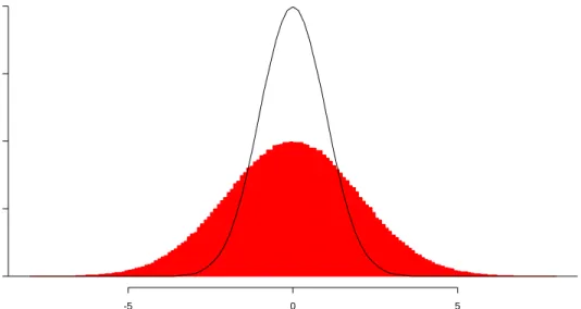
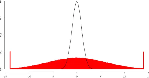
distributions based on the permutation and bootstrap resampling methods appear under the null hypothesis of equal means. For figures A-2 through A-7, two random samples of size five were generated, each from a normal distribution of mean 0 and standard deviation 1. The samples were resampled B = 100,000 times under each of the permutation and bootstrap methods. The resulting t-statistics from the 100,000 resamplings are shown as histograms with the true t distribution with 8 degrees of freedom overlaid. For figures A-8 through A-10 the sample sizes were increased from five per group to ten per group. It is readily apparent that the resampling based t -distributions differ substantially from the known t distribution, particularly for samples of size five. The permutation t distribution looks the least like the true distribution.
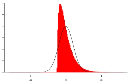
Because it is already well-known that the test based on the known t distribution is ideal for samples from identical normal distributions, figures A-11 through A-28 focus on the t-statistic null distributions when one of the underlying populations differs from standard normal. The figures are in groups of three. The first figure of a group (e.g., figure A-11) shows the underlying population distributions. The second figure (e.g., figure A-12) shows the true t-distribution based on 10,000,000 samples of size 5 from each of the distributions of the first figure. These are followed by a third figure (e.g., figure A-13) examining resampling based t-distributions created from single samples from the two distributions in question. Several underlying population distributions are examined in these figures ranging from differing variance to differing shape or both.
The non-normal distribution used is based on the Chi-Square distribution with 1 or 3 degrees of freedom. When the Chi-Square distribution is used, each value has the mean subtracted followed by division by the appropriate number to give the desired mean and variance.
The histograms of Appendix A illustrate some important aspects of the null distributions produced by the three resampling methods. First, the permutation and bootstrap across methods always generate a null distribution which is symmetric,
regardless of what the true null distribution should be. Second, the bootstrap within method and particularly the permutation method seem to produce distributions that are less stable than those produced by the bootstrap across method. Third, the true null t
distributions do not depart substantially from the common t distribution unless one of the underlying distributions is highly skewed.
2.2.4. Accuracy and Correctness
2.2.4.1. Definitions and ASL Formulation
This is a good point to discuss the concepts of accuracy and correctness, following the terminology of Efron and Tibshirani (1993). A test is accurate if
Prob(ASL≤α)=α when the null hypothesis is true, and
Prob(ASL≤α)= Expected Power
when the null hypothesis is false. The expected power is based on a known most powerful test. Thus, a test is accurate if the nominal level and power are preserved. A test is more accurate than another if Prob(ASL≤α) is closer to α under the null hypothesis and if Prob(ASL≤α) is closer to the expected power under the alternative hypothesis.
Correctness of a method indicates that the observed ASL is close to the P-value a
known optimal method would give for each data set. A test is more correct than another if it yields ASLs which are closer to the correct method P-values. Each correct method
P-value is based on a known distribution. For example, if two samples are known to come from normal distributions with equal variance, the known optimal method for comparing the means is the two-sample t-test. The t-statistics from this method are known to follow Student’s t distribution. For a given data set, ASLs from any other method (i.e., permutation test or bootstrap test) can be compared to the known correct P -value of the two-sample t-test. An ASL which is close to this P-value is more correct than an ASL which is further away.
Accuracy when the null hypothesis is false and correctness can only be evaluated for a method if a known most powerful test is available. It is for this reason that the bootstrap, permutation, and t-tests are first compared using samples with normal distributions of equal variance (of 1). The known Student’s t and noncentral t
distributions can be used to evaluate the bootstrap and permutation resampling methods for accuracy and correctness. For other null and alternative distributions (i.e., nonnormal or unequal variance), the unknown optimal test statistic distributions are estimated through simulation.
2.2.4.2. Estimated Test Size Comparison
A comparison of the estimated size for the two bootstrap methods, the permutation method, the known-size common t-test, and Welch’s t-test can be found in Appendix B. Each graph represents 20,000 simulated two-sample data sets. The means for the distributions from which each of the samples are taken are both zero, corresponding to the null hypothesis of equal means. Other parameters such as sample size in each group, variance, distribution types, and number of resamplings B are specific to each graph.
For the bootstrap and permutation tests, there are four possible definitions for the ASL. Because of the discrete nature of the compared sampling distributions, each definition may result in a different estimated size. The four definitions are
ASL=#(| |t* ≥ | |) /t B
ASL=#(|t*| > | |) /t B
ASL= +(1 #(| |t* ≥ | |)) /(1t +B) ASL= +(1 #(|t*| > | |)) /(1t +B)
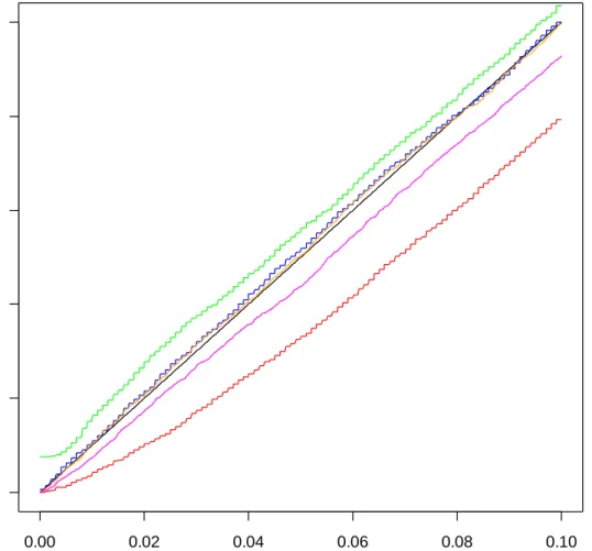
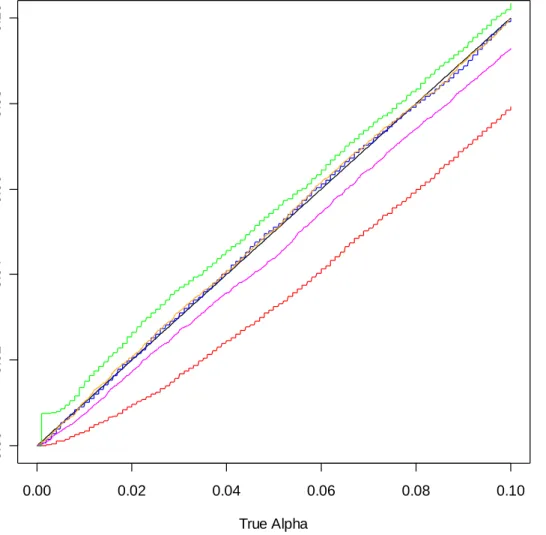
Figures B-1 through B-8 of Appendix B allow us to compare the effects of the definition of ASL and the choice of B. The graphs are created by finding the proportion of ASLs below small increments of alpha for each method and plotting them against those increments. The same 20,000 simulated data sets were used for all methods and for
all four definitions with B = 999 (figures B-1 through B-4). A new set of 20,000 simulated data sets was used for B = 1,000 (figures B-5 through B-8).
The choice of B and adding one to the numerator and denominator of the ASL definition appear to have very little effect on the estimated sizes. The estimated size based on the bootstrap across resampling method follows the t-test estimated size closely. When samples are of size 5 per group, the permutation method yields estimated sizes which are slightly below or slightly above the t-test estimated sizes, depending on whether equality is included in the ASL definition. Including equality produces the conservative result. For subsequent comparisons I use the definition of ASL:
ASL= +(1 #(| |t* ≥ | |)) /(1t +B)
because it is conservative for the small sample permutation method and since it is natural to include the observed t as one of the t*’s. Also, B = 999 will be used.
2.2.4.3. Two Sample Test Accuracy Comparison
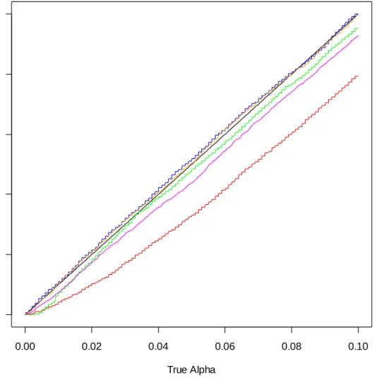
Figures B-9 through B-15 of Appendix B can be used to compare the accuracy of five tests: the standard t-test, Welch’s t-test, the permutation test, the within sample bootstrap test, and the across sample bootstrap test. The specifics of the distributions from which the samples are taken are shown below each graph. The black 45 degree line represents the true level. Estimated levels are given explicitly for known α = .01, .05, and .10 below each graph in a separate table of the appendix.
Welch’s t-test is seen to preserve the nominal error rate in all scenarios except those for which both the distribution shape and the variance of the two underlying distributions differ. The bootstrap within test is generally conservative while the permutation test, bootstrap across test, and t-test are general anti-conservative when the underlying distributions are not equal.
2.2.4.4. Power
The comparison of tests based on estimated power is done in the same way as that used for comparing estimated size, except that the means of the underlying
distributions from which the data are sampled are not equal. The results are found in Appendix C. The means differ by the amount shown below each graph. Here, again, the graphs are created by finding the proportion of ASLs below small increments of alpha and plotting them against those increments for each method. The same 20,000 simulated data sets are used for all methods. Care should be taken when interpreting these figures. Usually, the power of a test is evaluated for a given test size. In this case, the figures of Appendix B indicate that for many of the tests the size is very different from the nominal α. Power should be compared only after consulting the corresponding estimated size for the same test.
A comparison of the powers for the different tests follows a general trend of higher powers for the permuation, bootstrap across, and t-tests, although nominal sizes are seldom maintained for these tests. Welch’s t-test and the bootstrap within test are more conservative. This follows the pattern seen in the estimated sizes for the tests. Among the two tests which maintain the correct size for most distribution scenarios, Welch’s t-test clearly has higher power than the bootstrap within test. If little or nothing is known about the underlying distributions from which small samples are taken, or if the underlying distributions are known to differ in variance or distribution, Welch’s t-test is the recommended test based on accuracy and power.
2.2.4.5. Comparison of Correctness
We turn now from accuracy to correctness. Recall that correctness implies that the individual ASLs are close to the known correct P-values, where the known correct P-values are based on an optimal test. The correctness can be gauged by the mean square error of the observed ASLs from the known correct P-values for each method.
When the sampling distribution of the test statistic t is known, the P-value obtained from a specific realized t is obtained directly from that known sampling distribution. For example, suppose two samples of size 5 result in the two-sample test statistic t = 2.306. If this value is compared to Student’s t distribution with 8 degrees of freedom, the two-sided test P-value is 0.05. If two completely different samples result in
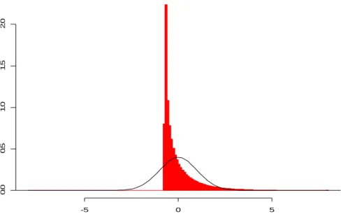
a test statistic that is also t = 2.306, the P-value for the test will still be 0.05. This is not the case when the sampling distribution of the test statistic is estimated from the data as in the bootstrap and permutation methods. Here, different samples typically result in different estimated sampling distributions. For example, using a resampling based distribution for t, an ASL for one two-sample data set with observed t = 2.306 may be 0.045 while for another two-sample data set with t = 2.306 the ASL might be 0.058, since the sample itself is used to create the sampling distribution. This concept can be visualized using the example shown in Figures 1-4. A single data set (of two samples) is used to produce all four graphs on the left of Figures 1-4, but by different methods. A similar data set is used to create all four graphs on the right. Each of the two data sets consists of two random samples of size five from a standard normal distribution. The histograms in the graphs represent the distribution used for each of the four methods for obtaining two-sided significance levels. In Figure 1, the distribution is the known Student’s t distribution. In Figures 2-4, the t distributions were created using bootstrap or permutation resampling. Each was produced from 10,000 resamples from each data set. If another 10,000 resamples were taken from the same data sets, the distributions would change. This change, however, may be considered negligible due to the finiteness of the number of permutation and bootstrap resamples when samples of size 5 are used (see Table 1), and because the number of resamples is substantial. Although the two data sets used in this example are random samples and do not result in t-statistics of 2.306, I assume that the resampled distributions of Figures 2-4 are typical of data sets which do result in a t-statistics of 2.306.
The objective of each of the bootstrap and permutation methods is to produce sampling distributions which are close to the known t distribution. In this example, this closeness in distribution to the known t distribution is determined by finding the proportion of the distribution outside -2.306 and 2.306. The correct proportion is known to be 0.05, based on the known Student’s t distribution with 8 degrees of freedom. The difference between the achieved proportion from each of the resampling based
distributions and the known proportion is a measure of the correctness of the method being used.
Student’s t distribution with 8 degrees of freedom
(a) (b)
Figure 1. First in a Series of Four Figures Depicting the Variation in Area Outside 2.306 When 4 Different Tests Are Used, t-distribution. The graph on the left represents a distribution from two samples of size five. The graph on the right represents another two samples. The same samples are used in Figures 1-4. The two-sided p-value for (a) is 0.025 + 0.025 = 0.05. The two-sided p-value for (b) is 0.025 + 0.025 = 0.05.
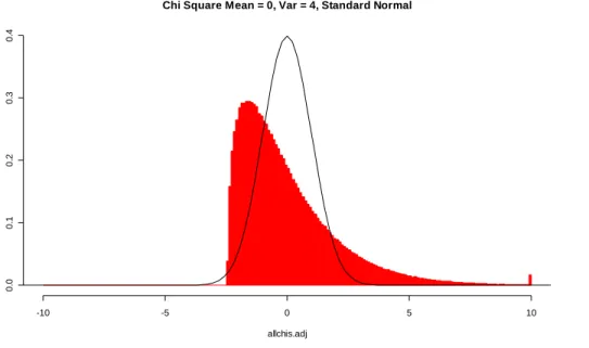
Permutation t Distribution two samples of size 5 (twice) (a) (b)
Figure 2. Second in a Series of Four Figures Depicting the Variation in Area Outside 2.306 When 4 Different Tests Are Used, Permutation Distribution. The left graph represents a distribution from two samples of size five. The right graph represents another two samples. The same samples are used in Figures 1-4. The two-sided ASL for (a) is 0.023 + 0.022 = 0.045. The two-sided ASL for (b) is 0.027 + 0.027 = 0.054.
single sample permutation t-distribution n = m = 5
perm.tstars De n s it y -6 -4 -2 0 2 4 6 0 .00 .1 0 .20 .3 0 .40 .5 0 .6
single sample permutation t-distribution n = m = 5
perm.tstars D ensi ty -6 -4 -2 0 2 4 6 0. 0 0 .1 0. 2 0 .3 0. 4 t-distribution df=8 t8 De n s it y t-distribution df=8 t8 De n s it y -2.306 2.306
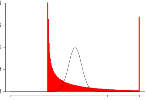
Bootstrap Within t distribution two samples of size 5 (twice) (a) (b)
Figure 3. Third in a Series of Four Figures Depicting the Variation in Area Outside 2.306 When 4 Different Tests Are Used, Bootstrap Within t Distribution. The graph on the left represents a distribution from two samples of size five. The graph on the right represents another two samples. The same samples are used in Figures 1-4. The two-sided ASL for (a) is 0.021 + 0.028 = 0.049. The two-two-sided ASL for (b) is 0.031 + 0.027 = 0.058.
Bootstrap Across t distribution two samples of size 5 (twice)
(a) (b)
Figure 4. Fourth in a Series of Four Figures Depicting the Variation in Area Outside 2.306 When 4 Different Tests Are Used, Bootstrap Across t Distribution. The graph on the left represents a distribution from two samples of size five. The graph on the right represents another two samples. The same samples are used in Figures 1-4. The two-sided ASL for (a) is 0.024 + 0.025 = 0.049. The two-two-sided ASL for (b) is 0.024 + 0.024 = 0.048.
single sample within group bootstrap t-distribution n = m = 5
boot.tstars.w D ens it y -6 -4 -2 0 2 4 6 0. 0 0 .1 0. 2 0 .3 0. 4
single sample across group bootstrap t-distribution n = m = 5
boot.tstars.a D ensi ty -6 -4 -2 0 2 4 6 0 .0 0 .1 0 .2 0 .3 0 .4
single sample within group bootstrap t-distribution n = m = 5
boot.tstars.w De n s it y -6 -4 -2 0 2 4 6 0. 0 0 .1 0. 2 0 .3 0. 4
single sample across group bootstrap t-distribution n = m = 5
boot.tstars.a D ens it y -6 -4 -2 0 2 4 6 0. 0 0 .1 0. 2 0 .3 0. 4
The graphs in Figures 1-4 illustrate the variation in ASL that occurs when a resampling method is used. Based on only two data sets, it appears that the bootstrap across t distribution is the most correct of the 3 resampling methods. The histograms in Figure 4 are closest to the correct distribution and the ASLs are closest to 0.05.
The results of a simulation study found in Appendix D show more rigorously the correctness of each of the methods for samples of size 5. First, 20,000 two-sample data sets were simulated from a normal distribution with mean zero and variance one. For each data set, the resampling distribution was produced using B = 999 resamples for each resampling method. Cutoff values for determining ASLs were chosen as seen in Table D-1, based on the known Student’s t distribution with 8 degrees of freedom. The correctness is measured as the mean square error of the ASLs from each known correct proportion (0.001, 0.01, 0.05, and 0.10). The most correct methods are those which yield the smallest mean square errors.
In Figure D-4 it is seen that the mean square error for the bootstrap across method is lowest, followed by the permutation method and then the bootstrap within method. This is the result anticipated based on the figures of Appendix A.
2.3. Two Sample Test Discussion and Recommendations
In terms of accuracy, for samples of size 5, the Welch’s t-test generally performs much better than the other methods. Except under the most extreme underlying distributions, Welch’s t-test preserves the nominal error rate. The bootstrap within test preserves the error rate but is usually far too conservative. The t-test, permutation test, and bootstrap across test are anti-conservative for even mild differences in shape or variance among underlying distributions. When the underlying distributions differ in both shape and variance, none of the examined tests is accurate for samples of size 5.
In terms of correctness, the ASL mean square error for the bootstrap across test is the lowest, followed by the permutation test. The ASL mean square error for the bootstrap within test is much higher than the other two.
Based on these simulation experiments, I recommend Welch’s t-test for a single test comparing the means of two samples of small sample size from unknown underlying distributions. If the underlying distributions are known to be at least close to normally distributed with equal variance, the common t-test is the preferred test because of the gain in power.
There is one other aspect of resampling based two-sample testing procedures that makes them undesirable, particularly when multiple comparison correction is to be done. The formula for an individual ASL is, again,
ASL= +(1 #(| |t* ≥ | |)) /(1t +B)
which has a minimum that is based on the size of B. That is, if B = 999, the smallest possible ASL is 1/(1 + 999) = 0.001. ASLs much smaller than this are required when hundreds or thousands of tests need be adjusted for simultaneously. The size of B is limited by the number of possible resampling permutations, which can be seen in Table 1.
Table 1 shows the number of unique resampling statistics that can be obtained from the three resampling methods for per group sample sizes of 2 to 10. If n is the sample size in each group, then the number of permutations as defined in Section 2.2.1 is given by 2n
n
⎛ ⎞
⎜ ⎟
⎝ ⎠. The numbers of unique bootstrap within and bootstrap across
resampling statistics as defined in Section 2.2.2 were derived to be 2n 1 2n 1
n n − − ⎛ ⎞⎛ ⎞ ⎜ ⎟⎜ ⎟ ⎝ ⎠⎝ ⎠ and 3n 1 3n 1 n n − − ⎛ ⎞⎛ ⎞ ⎜ ⎟⎜ ⎟ ⎝ ⎠⎝ ⎠, respectively.
Table 1. Number of Possible Unique Resampling Statistics from Three Resampling Methods for the Two Sample Test Scenario
Number of Obs. in
Each Group Permutation
Bootstrap Within Bootstrap Across 2 6 9 100 3 20 100 3,136 4 70 1,225 108,900 5 252 15,876 4,008,004 6 924 213,444 153,165,376 7 3,432 2,944,656 6,009,350,400 8 12,870 41,409,225 240,407,818,596 9 48,620 590,976,100 9,762,812,702,500 10 184,756 8,533,694,884 401,201,300,600,100
3. MULTIPLE TESTING ADJUSTMENT 3.1. Historical Perspective
Recognition for the need of appropriate adjustments in multiple testing has become widespread since the dissemination of the idea by Fisher (1935). A host of procedures have been developed to provide such adjustments for the various scenarios under which multiple testing occurs. Detailed treatment of most multiple comparison procedures can be found in Hochberg and Tamhane (1987) and Hsu (1996). Most multiple testing adjustment methods have centered around multiple testing in terms of the one-way layout scenario. However, with the increase in availability of data from increased computing power and novel techniques, multiple testing in more general situations with higher numbers of comparisons is occurring with greater frequency. When larger numbers of tests occur, more attention needs to be paid to issues such as bias, variance estimation, correlation, and distributional assumptions. That is, the effect of an incorrect assumption on the overall error rate for 20 – 30 tests may be only moderate while for 1000 tests the same incorrect assumption may affect the overall error rate dramatically.
To acquaint the reader with the development of multiple comparisons and testing in general, I offer a historical perspective and summary of the most commonly used procedures.
At the beginning of the nineteenth century, Legendre first proposed the minimization of the sum of squared errors as a method of estimating parameters (Legendre, 1805). This method, the method of least squares, was formalized shortly thereafter with the work of both Legendre and Gauss (Gauss, 1809). By around 1820, the concept of standard error and standard deviation as measures of variation emerged, largely due to the work of Laplace and Gauss (Cochran, 1976). Propelled by a desire to apply these and other mathematical tools to the social sciences, astronomy, agriculture, and later in studies of heredity, scientists throughout the 1800s made improvements and extensions to the method of least squares (Stigler, 1986). “It was this period which saw
the emergence and the beginning of the extensive use of the normal distribution both as a model and for approximating large-sample distributions of statistics and also the germination of seminal concepts like relative efficiency of estimators” (Chatterjee, 2003).
In the late nineteenth century, Sir Francis Galton, who is widely known for his work on the correlation coefficient, was asked by Charles Darwin for statistical advice concerning his height data for comparison of crossed and self-fertilized corn. Darwin had 15 replications for each group. Galton was aware that “averages of independent samples from a normal distribution are themselves normally distributed,” but did not feel comfortable estimating the standard deviation nor the “law of distribution followed by the individual differences in height” from only 15 observations (Cochran, 1976). In 1908, William Sealy Gossett, under the pen name of ‘Student’, published “The probable error of a mean” (Student, 1908) in which the sampling distribution of
s X n
t = ( −μ),
or ‘Student’s t’, was derived, paving the way for the legitimate comparison of means when only small samples are available. As was the case with many previous fundamental statistical discoveries of the eighteenth and nineteenth centuries, the value of this finding was not quickly disseminated. In 1922, Gossett wrote to R. A. Fisher, with whom he corresponded frequently, “I am sending you a copy of Student’s Tables as you are the only man that’s ever likely to use them!” (Cochran, 1976) It was Fisher who opened the door to comparative experimentation of multiple levels and factors with his work at Rothamsted Experimental Station and ensuing publication The Design of
Experiments (Fisher, 1935). In this cornerstone work, Fisher explained the now routine
techniques of blocking, randomization, factorial design, and the analysis of variance. In this same volume, Fisher also proposed two of the earliest methods for making appropriate adjustment for multiplicity of tests, which are often inherent with analysis of variance.
The suggestion of Fisher (1935) was to first test the effect of a factor using an overall F-test. If the F-test indicates significant differences among the means, it is
followed by individual t-tests, with the mean square error from the analysis of variance as the estimate of variance, comparing each mean to each other mean. This came to be know as the “protected” LSD (least significant difference), the protection coming, in his view, from the rejection of the F-test. If the F-test for equality of means is not deemed significant, Fisher proposed the conservative Bonferroni adjustment to the individual t -tests, also using the estimated variance based on the pooled samples.
Shortly thereafter, at the suggestion of Gossett (see Pearson, 1939) Newman (1939) proposed a method for comparing multiple means based on the studentized range. This method was modified by Keuls (1952), and came to be known as the Newman-Keuls (sometimes Student-Newman-Newman-Keuls) multiple range test (see Harter, 1980).
Increased interest in multiple comparison procedures following World War II was evidenced by the work of John W. Tukey, David B. Duncan, Henry Scheffe, and Charles W. Dunnett. Tukey (1952, 1953) presented another method based on the studentized range. The equal sample size version is now known as Tukey’s method or Tukey’s HSD (honest significant difference) method. For unequal sample sizes it is known as the Tukey-Kramer procedure (Kramer, 1956). A publication of Tukey (1953), a manuscript of mimeographed notes that has been widely circulated privately and widely used, was not produced until 1994 (Braun, 1994). Tukey (1953) proved that his equal sample size method maintains the overall experimentwise error rate. That is, the probability of a Type I error for all tests jointly, is α. Unable to prove this for differing
sample sizes, Tukey conjectured that the Tukey-Kramer procedure also preserved the overall experimentwise error rate (in the conservative direction). It was not until 1984 that Tukey’s conjecture was proven correct by Hayter (1984) (The Tukey-Kramer method was shown to be conservative based on simulation studies by Dunnett [1980]).
Duncan (1947, 1951, 1952, 1955) developed a multiple range test which by the late 1970s was the most commonly used multiple comparison procedure, according to a
Science Citation Index survey by Harter (1980). Duncan’s multiple range test has since
dropped in popularity based on the finding that it does not preserve the overall experimentwise error rate (see, for instance, Hsu [1996], pp. 129-130).
A method for jointly comparing all contrasts of means was developed by Scheffe (1953). Because this method is less powerful than Tukey’s method when only pair-wise comparison of means is desired, this method has come to be recommended only when the primary comparisons of interest are contrasts other than pair-wise comparisons.
Dunnett (1955) proposed a multiple comparison procedure similar to the Tukey methods, but for situations when only comparison with a single control is desired.
Development during the 1960s and 1970s in the areas of probability inequalities (i.e., Sidak’s (1967) inequality), unbalanced ANOVA methods, conditional confidence levels, empirical Bayes, and confidence bands in regression are outlined and discussed in Miller (1981). The empirical Bayes methods were set forth in a series of papers: Waller and Duncan (1969, 1974), Waller and Kemp (1975), Duncan (1975), and Dixon and Duncan (1975). The Ryan-Einot-Gabriel-Welsch (REGW) multiple range method was also developed during this period. Ryan (1960) proposed a conservative adjustment to α that was improved upon by Welsch (1972). This adjustment can be used in conjunction with the adjustment proposed by Einot and Gabriel (1975). Lehmann and Shaffer (1979) have shown this method “approximately maximizes the power subject to the [experimentwise error] control requirement” (for details, see Tamhane, 1995, pp. 607-610 or Hsu, 1996, pp. 128-129).
Multiple comparison procedures for finding the “best” treatment among several were developed by Hsu (1981, 1982) and Edwards and Hsu (1983) and improved in Hsu (1984). Comprehensive treatment of these developments can be found in Hsu (1996).
Because most of the above comparison procedures were developed for the one-way normal layout with equal variance model, distribution free and robust procedures for coping with nonnormal and heteroscedastic data were developed almost in parallel. It is well-known that t- and F- statistics are robust to non-severe departures from normality in the two-sample and one-way layout scenarios. However, as Hochberg and Tamhane (1987) note, “the problem of robustness becomes more serious in the case of multiple inferences.” Steel (1959a, 1959b) was the first to develop nonparametric multiple comparison procedures. Based on signs and ranks, these are applied to
comparison of means with a control when the assumption of normality is not met to permit use of Dunnett’s method. Similar all-pairwise nonparametric procedures based on signs and ranks were first developed and discussed in Steel (1960), Dwass (1960), Steel (1961), Nemenyi (1961), and Nemenyi (1963). The Kruskal-Wallis-type multiple comparison tests and similar tests (Friedman-type) for the two-way classification problem were also put forth in Nemenyi (1963). For a detailed description of the early development of nonparametric multiple testing procedures see Miller (1981).
More recently, Westfall and Young (1993) have applied the resampling ideas (such as the bootstrap first proposed by Efron [1979]) to the multiple comparison problem. Although computationally intensive, these methods are distribution-free, and can incorporate important correlation structure among the means.
Another perspective has found recent popularity in biological applications, particularly “gene finding.” Instead of preserving the experimentwise error rate for multiple comparisons, Benjamini and Hochberg (1995) proposed a different error rate, called the false discovery rate (FDR). I refer to the summary given in Tamhane (1995): “Let T and F be the (random) number of true and false null hypotheses rejected. Then the FDR is defined as FDR = E [T / (T + F)], where 0/0 is defined as 0. ... When all null hypotheses are true, the FDR equals [the experimentwise error rate]. … Since control of the FDR is less stringent than control of the [experimentwise error rate], it generally results in more rejections.”
3.2. Present Microarray Multiple Testing Problem
The following table (adapted to the subject of microarray data) is found in Benjamini and Hochberg’s (1995) false discovery rate article.
Table 2. Benjamini and Hochberg’s (1995) Table Used to Define the False Discovery Rate
Declared Declared
Not Different Different Total Genes in the treatment and control
groups are not differentially expressed U V m0
Genes in the treatment and control
groups are differentially expressed T S m – m0
m – R R m Note: The table is adapted to the subject of microarray data.
In Table 2, the null hypotheses for the microarray scenario are that the expression levels for the treatment and control groups for each gene are equal. The number m is the total number of hypotheses tested (or total number of genes) and is assumed to be known in advance. Of the m hypotheses tested, m0are true. The variable R is the total number of genes declared significantly different. The random variables U, V, T, and S are unobservable.
Individual P-values (or test statistics) are calculated for each test followed by adjustments to account for multiplicity of tests. It is desirable that these adjustments minimize the number of genes that are falsely declared different (V) while maximizing the number of genes which are correctly declared different (S). To address this issue the researcher must know the comparative value of finding a gene to the price of a false positive. If a false positive is very expensive, methods which focus on minimizing V should be used. If the value of finding a gene is much higher than the cost of additional false positives, methods which focus on maximizing S should be employed. Further, adjustments for multiplicity should incorporate to some degree the correlation of expressions of genes within an individual. There are groups of genes which are expressed in tandem while some genes may be “turned off” when others are “turned on.” Preferably, the method used to adjust for multiplicity of tests would incorporate an ability to account for this correlation.
Ge, Dudoit, and Speed (2003) outline the most common methods of control of false positive declarations:
• Per-comparison error rate (PCER), defined as PCER=E V( ) /m
• Per-family error rate (PFER), defined as PFER=E V( )
• Family-wise error rate (FWER), defined as FWER=Pr(V >0)
• False discovery rate (FDR) (Benjamini and Hochberg, 1995), defined as
{ 0} FDR ( 1R ) ( | 0) Pr( 0) V V E E R R R > R = = > >
• Positive false discovery rate (pFDR) (Storey, 2001, 2002), defined as pFDR E(V |R 0)
R
= >
These rates are generally considered to be computed under the complete null hypothesis of all genes being equally expressed between treatment and control groups. Ge, Dudoit, and Speed (2003) also show the following to be the general ordering of these rates:
PCER≤FDR≤pFDR≤FWER≤PFER
Dudoit, Shaffer, and Boldrick (2003) state, “Thus, for a fixed criterion α for controlling the Type I error rates, the order reverses for the number of rejections R: procedures that control the PFER are generally more conservative, that is, lead to fewer rejections, than those that control either the FWER or the PCER, and procedures that control the FWER are more conservative than those that control the PCER.”
A review and discussion of procedures which control the FWER can by found in Ge, Dudoit, and Speed (2003) and Dudoit, Shaffer, and Boldrick (2003). They describe in detail the following procedures for obtaining adjusted P-values:
1. Bonferroni single-step adjusted P-values 2. Sidak single-step adjusted P-values
3. Sidak step-down adjusted P-values 4. Holm step-down adjusted P-values 5. Single-step minP adjusted P-values 6. Step-down minP adjusted P-values 7. Single-step maxT adjusted P-values 8. Step-down maxT adjusted P-values
When single-step methods are used, the adjusted P-values may be used to reflect the amount of evidence of expression difference. That is, lower adjusted P-values indicate more evidence of a difference. Step-down method adjusted P-values can only be used to indicate a significant difference, but do not allow one to quantify the amount of evidence of a difference, except that the P-value is below the specified overall level that is to be preserved.
Adjusted P-values which control the FDR (Benjamini and Hochberg, 1995) are discussed in Ge, Dudoit, and Speed, (2003). Benjamini and Tekutieli (2001) proposed a modification to the Benjamini and Hochberg (1995) P-value adjustment which controls the FDR while allowing for arbitrary dependence. This method is considerably more conservative than the original method. Details of adjusted P-values (or q-values) based on the proposal of Storey (2001, 2002) are also found in Ge, Dudoit, and Speed (2003). 3.3. Details of Adjustment Methods Compared
3.3.1. Bonferroni Adjustment
The Bonferroni adjustment is applied to all m unadjusted P-values (pj) as min( ,1)
j j
p% = mp
3.3.2. Benjamini and Hochberg’s (1995) False Discovery Rate Control Procedure Adjusted P-values are found as
,..., min {min( ,1)} i k r r k i m m p p k = = % ,
where
1 2 m
r r r
p ≤ p ≤L≤ p are the observed ordered unadjusted P-values. The procedure is defined in Benjamini and Hochberg (1995). The corresponding adjusted P-value definition given here is found in Dudoit, Shaffer, and Boldrick, (2003).
3.3.3. Westfall and Young’s (1993) Single Step maxT Resampling Based Procedure The test statistics Tj are used to give adjusted P-values as
(
0)
1 Pr max | C j l j l m p T t H ≤ ≤ = ≥ % where 0 CH is the complete null hypothesis.
The Bonferroni and false discovery rate adjustment methods are two step methods. In the first step the unadjusted P-values are calculated. In the second step the error rate adjustment is made. In the case of the maxT resampling procedure, both steps are incorporated into a single process in the following way (Westfall and Young, 1993):
1. A counting variable is initial