DERIVING ANALYTICAL AXISYMMETRIC CROSS SECTION ANALYSIS AND COMPARING WITH FEM SIMULATIONS

DERIVING ANALYTICAL AXISYMMETRIC CROSS SECTION

ANALYSIS AND COMPARING WITH FEM SIMULATIONS

Magnus Komperød∗

Technological Analyses Centre Nexans Norway AS P. O. Box 42, 1751 HALDEN

Norway

ABSTRACT

Direct electrical heating (DEH) is a technology for preventing hydrate formation and wax deposit inside oil and gas pipelines. Nexans Norway AS is researching and developing deep-water DEH solutions. The company has already produced a deep-water DEH piggyback cable that can carry its own weight at 1 070 m water depth. When this DEH system is installed outside the coast of Africa, it will be the world’s deepest DEH system.

This paper derives axisymmetric cross section analysis calculations. The calculations are then ap-plied to the deep-water DEH piggyback cable and compared to finite element method (FEM) simu-lations of the same cable. There are very good agreements between the analytical calcusimu-lations and the FEM simulations. For three of five analysis results the differences are 0.6% or less. The largest difference is 4.2%, while the average difference (absolute values) is 1.8%.

Keywords:Axial Stiffness; Axisymmetric Analysis; Cross Section Analysis; DEH; Direct Electrical Heating; Offshore Technology; Subsea Cable; Torsion Stiffness.

NOTATION

A Cross section area of cable element

[m2].

E E-modulus of cable element [Pa].

~

Fc Load vector of the cable.

~

Fi Load vector of cable elementi.

G G-modulus (shear modulus) of cable

element [Pa].

Kc Stiffness matrix of the cable.

Ki Stiffness matrix of cable elementi.

L Pitch length of cable element [m].

l Length of cable element over one pitch length [m].

MT,c The cable’s torsion moment [Nm].

MT,i Contribution to the cable’s torsion mo-ment from cable elemo-menti[Nm].

R Pitch radius of cable element [m].

r Element radius of cable element [m].

∗_{Corresponding author: Phone: +47 69 17 35 39 E-mail:}

[email protected]

ri Inner element radius of cable element [m].

ro Outer element radius of cable element [m].

Tc The cable’s axial tension [N].

Ti Contribution to the cable’s axial ten-sion from cable elementi[N].

~uc Displacement vector of the cable and all cable elements.

V Volume of cable element [m3].

α Pitch angle of cable element [rad]. εc Axial cable strain [-].

εxx Axial element strain [-].

γxθ Shear strain in hoop direction on the surface perpendicular to the cylinder’s axis (length direction) [-].

ϕc Cable twist per cable unit length

[rad/m].

θ Angular position relative to the center

of the cable element [rad].

Π Potential energy of cable element [J].

Negative values ofLindicate left lay direction, and

positive values ofLindicate right lay direction. Sim-ilarly, negative values ofαindicate left lay direction,

and positive values ofα indicate right lay direction. All other length values are always positive.

INTRODUCTION

The world’s increasing energy demand, combined with the exhaustion of many easily accessible oil and gas reserves, drives the petroleum industry into deeper waters. Manufacturers of subsea cables and umbilicals are among those who face the technolog-ical challenges of increased water depths.

Another significant challenge of offshore petroleum production is that the pipeline content is cooled by the surrounding water. As the pipeline content drops to a certain temperature, hydrates may be formed and wax may start to deposit inside the pipeline wall. Hydrates and wax may partially, or even fully, block the pipeline. Hydrate formation may start at temper-ature as high as 25◦C, while wax deposit may start at 35-40◦C [1].

There are several ways to prevent hydrate forma-tion and wax deposiforma-tion. An intuitive soluforma-tion is to apply thermal insulation at the outer surface of the pipeline. However, at long pipelines, low flow rates, or production shut downs, this solution may be in-sufficient.

Depressurizing the pipeline content may be used to prevent hydrate formation. However, at deep-water pipelines, high pressure is required to bring the pipeline content to topside. Plug removal by de-pressurizing also faces the same problem at deep-water pipelines [2].

When thermal insulation and depressurizing are in-sufficient, a commonly used approach is to add chemicals to the pipeline in order to reduce the criti-cal temperature for hydrate formation and wax de-position. Methanol or glycol is commonly used [1, 3]. However, as explained in reference [1], adding chemicals has practical as well as environ-mental disadvantages.

Another approach to prevent hydrate formation and wax deposition is to use power cables inside the ther-mal insulation of the pipeline. The power cables function as heating elements heating the pipeline. However, embedding the cables inside the thermal insulation may lead to practical difficulties [1]. A technology that has emerged over the last years is direct electrical heating (DEH). The first DEH

sys-tem was installed at Statoil’s Åsgard oil and gas field in the Norwegian Sea in year 2000 [4]. Nexans Nor-way AS qualified the DEH technology together with Statoil and SINTEF.

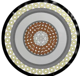
In DEH systems, the electrical resistance of the steel in the pipeline wall is used as a heating element. A single phase cable, referred to as piggyback cable (PBC), is strapped to the pipeline. In the far end (the end of the pipeline far away from the topside) the PBC is connected ("short circuited") to the pipeline. In the near end (the end of the pipeline close to the topside), a two-phase DEH riser cable is connected to the PBC and the pipeline; one phase of the riser cable is connected to the PBC, and the other phase of the riser cable is connected to the pipeline. When the riser cable is energized topside, energy is transferred through the PBC into the steel of the pipeline wall. Nexans Norway AS is currently developing deep-water DEH solutions. A piggyback cable that is reparable, i.e. can carry its own weight, at 1 070 m water depth is already produced by Nexans in a de-livery project. The cross section of this cable is shown in Figure 1. When this DEH system is in-stalled outside the coast of Africa, it will be the world’s deepest DEH system [4].

Figure 1: Cross section of the deep-water DEH pig-gyback cable.

The piggyback cable shown in Figure 1 has 19 (1 + 6 + 12) steel strands in center (gray color in the fig-ure). The purpose of the steel strands is to improve the mechanical capacity of the conductor. This so-lution is patented by Nexans Norway AS. Outside the steel strands there are 72 (18 + 24 + 30)

per strands (brown color). Outside the stranded con-ductor there are an electric insulation system (dark gray and light gray colors) and an inner sheath (gray color). Outside the inner sheath there are fillers for mechanical protection (yellow color), and then the outer sheath (black color).

The contribution of this paper is to derive analytical calculations for axisymmetric analysis of the deep-water DEH piggyback cable presented in Figure 1, and compare these analysis results with finite ele-ment method (FEM) simulations of the same cable. Analytical calculations increase the analysts’ theo-retical and practical understanding compared to us-ing FEM tools. Analytical calculations are also very efficient, both in terms of man-hours and CPU time. The analytical derivations presented in this paper are strongly inspired by references [5] and [6].

CROSS SECTION ANALYSIS AND AXI-SYMMETRIC ANALYSIS

The term cross section analysis refers to a set of analyses on cables, including umbilicals, that de-scribes the cables’ mechanical properties. Nexans Norway AS usually includes the following analyses in cross section analyses of DEH cables and umbili-cals:

• Axial stiffness when the cable is free to twist [N].

• Axial stiffness when the cable is prevented from twisting [N].

• Bending stiffness [Nm/(m−1)].

• Torsion stiffness [Nm/(rad/m)].

• Torsion angle to axial tension ratio when the cable is free to twist [(rad/m)/N].

• Torsion moment to axial tension ratio when the cable is prevented from twisting [Nm/N].

• Capacity during installation.

• Capacity during operation.

The cable’s capacity refers to allowed combinations of axial tension [N] and bending curvature [m−1]. Cross section analyses can be done by analytical calculations or by FEM simulations. Reference [5]

gives an excellent introduction to the theoretical fun-dament for analytical calculations. Several other publications, for example references [6] and [7], also cover parts of this theory.

There also exist commercial available software tools for performing cross section analyses. Both ware tools based on analytical calculations and soft-ware tools based on FEM simulations are available. The term axisymmetric analysis refers to a subset of those analyses included in the cross section analysis. Axisymmetric analysis includes exactly those anal-yses where the cable is straight (not bent):

• Axial stiffness when the cable is free to twist [N].

• Axial stiffness when the cable is prevented from twisting [N].

• Torsion stiffness [Nm/(rad/m)].

• Torsion angle to axial tension ratio when the cable is free to twist [(rad/m)/N].

• Torsion moment to axial tension ratio when the cable is prevented from twisting [Nm/N]. As will be shown in this paper, the analyses in-cluded in the axisymmetric analysis are mathemat-ically closely related and can be derived from the same stiffness matrix.

DERIVATION OF AXISYMMETRIC ANALY-SIS

The derivation presented in this section is strongly inspired by references [5] and [6]. The following assumptions and simplifications apply: (i) Friction is neglected. This is a common assumption in ax-isymmetric analysis, see for example reference [7]. (Please note that friction is important in the non-axisymmetric part of the cross section analysis.) (ii) Linear elastic materials are assumed. (iii) Radial dis-placement is neglected. (iv) The Poisson ratio effect is neglected. (v) Helical elements are modeled as tendons. That is, the elements have axial stiffness in tension and compression, while torsion stiffness and bending stiffness are neglected. Please note that the helical elements’ influence on the cable’s tor-sion moment and tortor-sion stiffness is included in the model.

From the author’s point of view, assumption (i) is probably correct for axisymmetrical analysis in gen-eral. The other assumptions must be used with care. In some cases these assumptions have negligi-ble influence on the analysis results, while in other cases they may introduce significant inaccuracy. As shown later in this paper, the analytical calculations give very good agreements with FEM simulations for the deep-water DEH piggyback cable presented in Figure 1. Hence, the applied assumptions do not significantly deteriorate the accuracy of the calcula-tions.

As seen from Figure 1, the cable elements of the PBC can be divided into two types: (i) Non-helical cylinders. Those are the electric isolation system, the inner sheath, and the outer sheath. (ii) Helical elements. Those are the strands of the conductor, as well as the protection fillers. (The center strand of the conductor is modeled as a helical element with zero pitch radius.)

In the axisymmetric case, i.e. when the cable is straight (not bent), the cable has two degrees of free-dom: Axial strain,εc, and twist per cable unit length, ϕc. These variables are stacked in a vector to form

the displacement vector~uc = [εc,ϕc]T. The cor-responding loads are: Axial tension, Tc, and tor-sion moment, MT,c. The load vector is then ~Fc =

[Tc,MT,c]T. The stiffness matrix, Kc, relates the displacement vector and the load vector

~ Fc=Kc~uc (1) Tc MT,c = kc,11 kc,12 kc,21 kc,22 εc ϕc .

As will be explained later in this paper, the displace-ment vector,~uc, is common for all cable elements, as well as for the cable itself. The load vectors and the stiffness matrices are individual to each cable ele-ment. The load vector of cable elementiis~Fi, while the load vector of the cable is~Fc. Similarly, the stiff-ness matrix of cable elementiisKi, and the stiffness matrix of the cable isKc. The following text derives the stiffness matrices for cylinder cable elements and for helical cable elements.

Stiffness Matrix of a Cylinder Cable Element Subject to the degrees of freedom presented above, the potential energy, Π, of a non-helical cylinder

over an axial lengthLcan be expressed as

Π(εc,ϕc) = Z V 1 2Eεxx 2₊1 2Gγxθ 2 dV (2) −TiLεc−MT,iLϕc.

The last two terms of Eq. 2 are the potential energy of the applied loads. The first expression in the in-tegration term of Eq. 2 is the strain energy in the cylinder due to axial tension. As the cylinder is non-helical, the axial strain of the cylinder,εxx, is equal to

the axial strain of the cable,εc. Also, the axial strain is equal over the cylinder volume. This simplifies to

Z V 1 2Eεxx 2_{dV =}1 2Eεc 2Z V dV (3) =1 2Eεc 2 L Z 0 2π Z 0 ro Z ri rdrdθdL =π 2EL(ro 2_−r i2)εc2.

The second term in the integration term of Eq. 2 is the strain energy in the cylinder due to torsion. A simple geometric consideration shows that the shear strain, γxθ, is given byγxθ =rϕc. Asϕcis constant over the cable volume, it follows that

Z V 1 2Gγxθ 2_{dV =}Z V 1 2Gr 2 ϕc2dV (4) =1 2Gϕc 2Z V r2dV =1 2Gϕc 2 L Z 0 2π Z 0 ro Z ri r2rdrdθdL =π 4GL(ro 4_−r i4)ϕc2. Eq. 2 can then be rewritten as

Π(εc,ϕc) = π 2EL(ro 2_−r i2)εc2 (5) +π 4GL(ro 4_−r i4)ϕc2 −TiLεc−MT,iLϕc.

The cable is in equilibrium when the potential en-ergy, Π, is at a stationary point. The equilibrium

conditions are then

∂Π(εc,ϕc) ∂ εc =πEL(ro2−ri2)εc−TiL=0, (6) ∂Π(εc,ϕc) ∂ ϕc =π 2GL(ro 4_−r i4)ϕc−MT,iL=0. (7) Dividing Eq. 6 and Eq. 7 byLgives

Ti=πE(ro2−ri2)εc, (8) MT,i= π 2G(ro 4_−r i4)ϕc. (9) The stiffness matrix of a cylinder cable element is then given by ~ Fi=Ki~uc (10) Ti MT,i = πE(ro2−ri2) 0 0 π 2G(ro 4_−r i4) εc ϕc .

Stiffness Matrix of a Helical Cable Element As stated above, the helical cable elements are mod-eled as tendons. This means that these elements’ bending stiffness and torsion stiffness are neglected. The helical element’s potential energy over a pitch length,L, is then Π(εc,ϕc) = Z V 1 2Eεxx 2_{dV (11)} −TiLεc−MT,iLϕc.

The last two terms of Eq. 11 are the potential energy of the applied loads. The integration term of Eq. 11 is the strain energy in the helical element due to its axial strain. Because bending stiffness and thereby strain from bending are neglected, the axial strain is equal over the element’s volume. Hence, the strain energy can be written as

Z V 1 2Eεxx 2_{dV =}1 2Eεxx 2Z V dV (12) =1 2Eεxx 2 l Z 0 2π Z 0 r Z 0 rdrdθdl =π 2Elr 2 εxx2 =1 2 EAL cos(α)εxx 2

In the last line of Eq. 12, it is used thatA=πr2and l =L/cos(α). As for the cylinder case, the

heli-cal element is in equilibrium when the potential en-ergy,Π, is at a stationary point. Inserting Eq. 12 into

Eq. 11 and differentiating gives

∂Π(εc,ϕc) ∂ εc = EAL cos(α)εxx ∂ εxx ∂ εc −TiL=0, (13) ∂Π(εc,ϕc) ∂ ϕc = EAL cos(α)εxx ∂ εxx ∂ ϕc −MT,iL=0. (14)

The next issue is to deriveεxx as function ofεc and

ϕc. While helical elements are three dimensional ge-ometries, it is common to illustrate these geometries in two dimensions as shown in Figure 2. The pitch length,L, is the axial length of the cable correspond-ing to one revolution of the helix. Elements in the same cable layer always have the same pitch length. The element length, l, is the length of the cable el-ement over one pitch length. The pitch radius,R, is the radius from center of the cable to center of the element. The pitch angle, α, is the angle between

the cable’s axis (length direction) and the tangent of the helix. Figure 2 shows the geometric relation be-tween L, R, θ, l, and α. This relation is true for θ =2πrad.

R θ

L _l

α

Figure 2: Geometric relation betweenL,l,R,θ, and α. The relation it true forθ=2π rad.

Based on Figure 2, Pythagoras’ theorem gives

l2=L2+ (Rθ)2. (15)

Differentiation of Eq. 15 and division by 2l2gives

dl l = LdL l2 + R2θdθ l2 . (16)

In Eq. 16, Ris a constant. Insertingl=L/cos(α), l=Rθ/sin(α), andθ=2πrad gives

dl l =cos 2₍ α)dL L +sin 2₍ α)dθ 2π, (17) εxx=cos2(α)εc+sin2(α) L 2πϕc, (18)

εxx=cos2(α)εc+Rcos(α)sin(α)ϕc. (19) In Eq. 18 it has been used thatεxxdef=dl/l,εcdef=dL/L, and dθ =Lϕc. In Eq. 19 it has been used that

tan(α) =2πR/L. Inserting Eq. 19 and its partial derivatives into Eq. 13 and Eq. 14, and dividing the latter equations withLgives

Ti=EAcos3(α)εc (20)

+EARcos2(α)sin(α)ϕc,

MT,i=EARcos2(α)sin(α)εc (21)

+EAR2cos(α)sin2(α)ϕc.

The stiffness matrix for helical elements is then

~ Fi=Ki~uc (22) Ti MT,i = ki,11 ki,12 ki,21 ki,22 εc ϕc , ki,11=EAcos3(α),

ki,12=ki,21=EARcos2(α)sin(α), ki,22=EAR2cos(α)sin2(α).

Stiffness Matrix of Cable

The previous sections derive the stiffness matrices of non-helical cylinder elements and helical elements. This section explains how to calculate the stiffness matrix of the cable based on stiffness matrices of the cable elements.

All cable elements, as well as the cable itself, are subject to the same strain along the cable’s length direction, εc, and the same twist along the cable’s axis, ϕc. Hence, they all share the same

displace-ment vector~uc= [εc,ϕc]T.

The axial tension of the cable, Tc, is equal to the contributions from all cable elements, ∑iTi. Simi-larly, the torsion moment of the cable,MT,c, is equal

to the contributions from all cable elements,∑iMT,i. Therefore, the cable’s load vector is equal to the sum of the load vectors of all cable elements. That is

~ Fc=

∑

∑

∑

Comparison in the second row of Eq. 23 proves that the stiffness matrix of the cable, Kc, is equal to the sum of the stiffness matrices of all cable elements, i.e.

Kc=

∑

Ki. (24)

Computing Axisymmetric Analysis Results The previous section shows how to compute the ca-ble’s stiffness matrix. This section explains how to compute the axisymmetric analysis results from the stiffness matrix. The stiffness matrix is on the form

Tc MT,c = kc,11 kc,12 kc,21 kc,22 εc ϕc . (25) Note that kc,12 =kc,21, both for non-helical

cylin-ders, for helical elements, and hence for the cable itself. It is in this context more convenient to write the matrix as a set of linear equations, where it is used thatkc,12=kc,21. That is

Tc=kc,11εc+kc,12ϕc, (26)

MT,c=kc,12εc+kc,22ϕc. (27)

The following sections derive the axisymmetric re-sults. Please note that the stiffness matrix of the ca-ble must be calculated first, using Eq. 24, and then be

used in the calculations presented below. The oppo-site, i.e. to first compute the axisymmetric analyses for each cable element, and then sum these analyses to obtain the analysis for the cable will give erro-neous results (except for in some special cases).

Axial Stiffness at Free Twist

When the cable is free to twist, it does not set up any torsion moment. InsertingMT,c=0 into Eq. 27, solving forϕc, and inserting this into Eq. 26 gives

Tc= kc,11− kc,122 kc,22 εc. (28)

Hence, the axial stiffness at free twist iskc,11−

kc,122 kc,22.

Axial Stiffness at No Twist

No twist is equivalent toϕc=0. Inserting this into Eq. 26 givesTc=kc,11εc. Hence, the axial stiffness

at no twist iskc,11.

Torsion Stiffness at Free Elongation

Solving Eq. 26 forεc and inserting this into Eq. 27 gives MT,c(Tc,ϕc) = kc,12 kc,11 Tc+ kc,22− kc,122 kc,11 ϕc, (29) ∂MT,c(Tc,ϕc) ∂ ϕc =kc,22− kc,122 kc,11 . (30)

Hence, the torsion stiffness at free elongation is

kc,22−

kc,122

kc,11. Please note that in Eq. 29 and Eq. 30,

MT,c is a function ofTc andϕc, not a function ofεc as in the other cases.

Torsion Angle to Axial Tension Ratio

In this case, the cable is free to twist, i.e. it sets up no torsion moment. InsertingMT,c=0 into Eq. 27, solving forεc, and inserting this into Eq. 26 gives

Tc= −kc,11kc,22 kc,12 +kc,12 ϕc, (31) ϕc Tc = kc,12 kc,122−kc,11kc,22 . (32)

Hence, the torsion angle to axial tension ratio is kc,12

kc,122−kc,11kc,22.

Torsion Moment to Axial Tension Ratio

In this case, the cable is prevented from twisting. Insertingϕc=0 into Eq. 26 and Eq. 27, and solving both equations forεcgives

εc= Tc kc,11 =MT,c kc,12 , (33) MT,c Tc =kc,12 kc,11 . (34)

Hence, the torsion moment to axial tension ratio is kc,12

kc,11.

UFLEX2D

The UFLEX program system originates from a joint Marintek and Nexans effort kicked off in 1999, resulting in a 2D software module (UFLEX2D) for structural analysis of complex umbilical cross-sections. The first version of the tool was launched in 2001. From 2005 and onwards further develop-ment of the 2D module as well as the developdevelop-ment of a 3D module (UFLEX3D) has taken place within a Joint Industry Project (JIP). The JIP is still run-ning, and is financed by a group of 10 sponsors cov-ering the following oil and gas industry segments; operators, suppliers, technical service providers. UFLEX2D is a finite element method (FEM) tool, which can be used to simulate all analysis results that Nexans Norway AS includes in cross section

analyses. Figure 3 shows the UFLEX2D FEM

model of the deep-water DEH piggyback cable pre-sented in Figure 1.

COMPARING ANALYTICAL CALCULA-TIONS WITH FEM SIMULACALCULA-TIONS

Table 1 presents the differences of the analytical cal-culations derived in this paper and the results of the UFLEX2D FEM simulations. The table shows that there are very good agreements between the analyti-cal analyti-calculations and the FEM simulations. For three of the five results the differences are 0.6% or less. The largest difference is 4.2%. The average differ-ence (absolute values) is 1.8%.

Figure 3: Finite element model of the deep-water DEH piggyback cable. The colors of the figure do not represent any physical values.

Analysis Result Difference[%]

Axial stiffness (free twist) 0.6

Axial stiffness (no twist) 0.3

Torsion stiffness (free elonga-tion)

−3.8 Torsion angle to axial tension

ra-tio

4.2 Torsion moment to axial tension

ratio

0.0

Table 1: Differences between analytical calculations and UFLEX2D FEM simulations.

Based on the good agreements between the analyti-cal analyti-calculations and the FEM simulations, it is con-cluded that the analytical derivations presented in this paper cover the significant physical effects of the deep-water DEH piggyback cable. Further it is concluded that the applied assumptions and simplifi-cations do not significantly deteriorate the accuracy of the calculations.

CONCLUSIONS

This paper derives analytical calculations for axi-symmetric analyses. These calculations have been used to compute the axisymmetric analysis results for a deep-water DEH piggyback cable developed by Nexans Norway AS. This piggyback cable is repara-ble, i.e. can carry its own weight, at 1 070 m water

depth. The development of the piggyback cable is part of Nexans’ efforts towards deep-water DEH so-lutions.

The analytical calculations are compared to

UFLEX2D FEM simulations. There are very good agreements between the analytical calculations and the FEM simulations. For three of the five analysis results the differences are 0.6% or less. The largest difference is 4.2%, while the average difference (absolute values) is 1.8%.

REFERENCES

[1] A. Nysveen, H. Kulbotten, J. K. Lervik, A. H. Børnes, M. Høyer-Hansen, and J. J. Bremnes. Direct Electrical Heating of Subsea Pipelines -Technology Development and Operating Expe-rience. IEEE Transactions on Industry Applica-tions, 43:118 – 129, 2007.

[2] J. K. Lervik, M. Høyer-Hansen, Ø. Iversen, and S. Nilsson. New Developments of Direct Elec-trical Heating for Flow Assurance. In Proceed-ings of the Twenty-second (2012) International Offshore and Polar Engineering Conference -Rhodes, Greece, 2012.

[3] S. Dretvik and A. H. Børnes. Direct Heated Flowlines in the Åsgard Field. InProceedings of the Eleventh (2001) International Offshore and Polar Engineering Conference - Stavanger, Nor-way, 2001.

[4] S. Kvande. Direct Electrical Heating Goes Deeper. E&P Magazine June 2014, 2014.

[5] E. Kebadze. Theoretical Modelling of

Un-bonded Flexible Pipe Cross-Sections. PhD the-sis, South Bank University, 2000.

[6] R. H. Knapp. Derivation of a new stiffness ma-trix for helically armoured cables considering tension and torsion. International Journal for Numerical Methods in Engineering, 14:515 – 529, 1979.

[7] N. Sødahl, G. Skeie, O. Steinkjær, and A. J. Kalleklev. Efficient fatigue analysis of helix el-ements in umbilicals and flexible risers. In Pro-ceedings of the ASME 29th International Con-ference on Ocean, Offshore and Arctic Engi-neering OMAE 2010, 2010.