CDO mapping with stochastic recovery
Andrea Prampolini
HSH Nordbank AG
∗155 Moorgate, London EC2M 6UJ, UK
[email protected]
Matthias Dinnis
HSH Nordbank AG
Schloßgarten 14, 24103 Kiel, Germany
[email protected]
19 February 2009
Abstract
We discuss in detail the mapping methodology for the valuation of be-spoke single tranche Collateralized Debt Obligations in the context of the stochastic recovery gaussian factor modelling framework recently proposed by Amraoui and Hitier [1].
1
Introduction
A Collateralized Debt Obligation (CDO) provides tranched exposure to an underlying portfolio of obligors. The market for CDOs is relatively young, dating back to the late 1990s [12]. In 2003 a liquid market for standard index tranches was initiated, although interest in the products gained mo-mentum only from late 2004. One of the main drivers for creating such a liquid market was the need on the part of the dealers to hedge their exposure in the bespoke single tranche CDO business [8]. As a corollary, standard tranches would also reflect the market’s view on credit correla-tion so that they could be used as a benchmark for pricing bespoke deals. It is therefore clear that one of the problems which was present since the beginning of the standard tranche market was how to extract the correla-tion informacorrela-tion contained in the price of liquid instruments and use it to evaluate and risk manage bespoke tranches.
∗
The views expressed are the authors’ own and not necessarily those of HSH Nordbank. We are grateful for valuable feedback from Damiano Brigo, Bernd Lewerenz and Marco Tarenghi.
2
Correlation market shocks and the normal
copula
In its short history, the credit correlation market faced two major crises: one of idiosyncratic nature in May 2005, while the other, principally of sys-temic nature and much more severe in intensity, started in July 2007 and was still ongoing at the time of writing this paper. At the onset of both crises, the most widely used model for pricing standard tranches was the one factor normal copula with deterministic recovery [3] [18], which will be referred to in the following as the ‘standard’ model. The value of the de-terministic recovery parameter was either set at a value of 40% coherently with CDS index conventions, or it was set for each entity to the relevant recovery value as published by Markit. In May 2005 implied base correla-tions dropped sharply as a result of the downgrade to sub-investment grade of General Motors and Ford by S&P, reflecting heightened concerns about the possibility of a major isolated default. In July 2007, a sharp increase in delinquencies among US subprime residential borrowers was the epicentre of seismic waves of repricing that were dubbed the ‘credit crunch’ in the light of a sharp tightening of liquidity conditions in the capital markets; in particular implied correlation levels in the standard tranche markets soared to unprecedented highs as dealers feared that default contagion and an impending depression might trigger a large number of insolvencies in the global credit markets. The problem with the credit crunch, and a differ-ence between the two crises, was that while for the 2005 crisis the repricing could be captured by the standard model, during the more recent turmoil the normal copula proved inadequate to explain the new levels reached by the supersenior tranches in particular. As a consequence, market players (and particularly investors) suffered a crisis of confidence in the mainstream modelling framework, which wasn’t able to attain market prices any longer as implied correlations hit the 100% ceiling.
In particular, the deterministic recovery assumption appeared inade-quate in light of the fact that it shielded from loss a whole portion of the capital structure (see the discussion on the ‘super-duper tranche’ in [1]). Dealers reacted first with deterministic mark-downs (ie. by lowering recovery rate assumptions when pricing tranches in the senior part of the capital structure, with the result of creating a ‘recovery skew’ in an analogy with the correlation skew), then they looked at adding stochastic recovery features to their modelling approaches.
Although many alternative dependence specifications have been pro-posed by academia and practitioners, the standard model indisputably had a major influence in creating a common language for the credit correla-tion market, especially for investors. Relaxing the deterministic recovery assumption appears to be a sensible step in the light of evolving market consensus.
3
Payoff
In this section we introduce our notation for the payoff of a single tranche CDO.
Call U the finite set of all defaultable entities in an economy. Two random variables are associated with each entity i ∈ U: a default time
τi>0 and a (stationary) recovery rateRiwhich maps the sample space to
[0,1]. A (static) pool is a finite setP of nonnegative real numbers{wi}i∈C
indexed on a subsetC ofU, with the condition that
X
wi∈P
wi= 1 (1)
Each element inP is associated with a reference entity, so that condition (1) means that entity weightings in the pool must add up to 1. The loss process on the pool at timetis given by
LP(t) = X
wi∈P
1τi<twi (1−Ri) (2)
We may refer to the quantity
LGDi:=wi(1−Ri) (3)
as the loss given default in the portfolio associated with entity i. Let us also define the portfolio recovery process
RP(t) = X
wi∈P
1τi<twiRi (4)
and the process for the outstanding notional of the pool
NP(t) = 1−LP(t)−RP(t) (5)
We first define the discounted payoff B(d, T) of a 0-d tranche (‘base tranche’) onP with detachment point (‘strike’)d∈(0,1] and maturityT. We start by specifying (terminal) loss, recovery and outstanding notional processes for the base tranche (we drop theP subscript for simplicity):
Ld(t) = min (LP(t), d) (6) Rd(t) = max (0, RP(t) +d−1) (7) Nd(t) =d−Ld(t)−Rd(t) (8)
The base tranche is composed of two legs: a premium leg and a protec-tion leg. The discounted payoff of the base tranche protecprotec-tion leg is
BaseProtection(d, T) :=
Z T
0
D(0, t)dLd(t) (9)
and that of the premium leg is
BasePremium(d, T) :=S0 b X k=1 D(0, Tk) Z Tk Tk−1 Nd(t)dt (10)
From the point of view of the protection buyer we can write
B(d, T) :=BaseProtection(d, T)−BasePremium(d, T) (11) to which the payment of any upfront amounts (usually exchanged on the third business day after trade date) should be added.
A Single Tranche CDO can be constructed as the difference of two base tranchesB(a, T) andB(d, T), whereais the attachment point of the tranche anddis the detachment point. Again from the point of view of the protection buyer we can write
STCDO(a, d, T) =B(d, T)−B(a, T) (12) There are special pools that represent the traded CDS indices for which a set of standard tranches exists. We callPEUsthe pool of the iTraxx
Eu-rope Seriessindex and PNAsthe pool of the CDX North America
Invest-ment Grade Seriess. Standard tranches on these pools will beBEUs(d, T) andBNAs(d, T) respectively.
Given a model of the loss and notional processes for the pool, the risk neutral expected value of the discounted payoffs defined in this section can be calculated. In the next section we review the model that we’ll be using in this paper.
4
Portfolio loss model
The portfolio loss and recovery processes have been defined in equations (2) and (4) in terms of individual default times and recovery rate random variables. The conventional setting for mapping methods is the ‘standard’ normal copula framework, ie a one factor normal copula model with de-terministic recovery. More in detail, multivariate default events up to a given time horizonT are driven by a set of (|P|+ 1) iid∼ N(0,1) random variablesZ,{Zi}, which are given a factor structure by defining
Xi = √ ρiZ+ p 1−ρiZi i= 1. . .|P| (13) such that pi :=E[1τi<T] =P[Xi<N −1(p i)] (14)
Probabilitiespiare extracted from single name Credit Default Swap (CDS)
market prices. Bivariate correlations for the resulting copula of default times are given by√ρiρj for entitiesi6=j. This model benefits from well
known semi-analytic algorithms for calculating the portfolio loss distribu-tion (see for instance [3] and [13]).
To overcome the calibration issues discussed in Section 2, we extend the standard normal copula framework by relaxing the deterministic re-covery assumption along the lines of [1]. This can be done by retaining at the same time the semi-analytical tractability of the standard model as detailed in Section 4.1. The Amraoui-Hitier extension is particularly ap-pealing because it’s a fully stochastic specification of recovery rates which remains consistent with single name and index pricing. Recovery Ri is
factorZ (recall thatZ is the inverse normal of a uniform random variable:
Z=N−1(U)). The functionR
i(z) is defined by the following equation (see
equation (2) on page 6 of the Amraoui-Hitier paper):
Ri(z) = 1− 1−R˜i N N−1( ˜p i)−√ρiz √ 1−ρi NN−1√(pi)−√ρiz 1−ρi (15)
where ˜Ri and ˜pi are linked via
˜
pi=
1−R¯i
1−R˜i
pi (16)
which preserves conditional expected loss. ¯Ri is the deterministic recovery
used to bootstrap the single name CDS curve default probabilities for entity
i. Composite quotes for the value of ¯Rifor most liquid entity are published
daily by Markit. ˜Riis a free parameter that must be chosen by the modeller;
it represents the minimum value of the distribution domain forRi(z), in
other words the stochastic recovery for entityitakes values in [ ˜Ri,1]. Our
preferred choice for the value of ˜Ri is zero, especially in the light of the
results of recovery auctions in 2008 [7]. Otherwise, if one chooses a positive value for ˜Rithere will always be a portion (however small) of the underlying
pool that will be shielded from default by construction. Only the possibility to attain a full armageddon scenario (see also [19]) effectively eliminates the ‘super-duper tranche’ issue.
We observe that the copula of default events is preserved by the Amraoui-Hitier extension: pi|z=E[1τi<T |Z=z] =N N−1(p i)− √ ρiz √ 1−ρi (17) so that conditional probabilities can still be computed semi-analytically.
In terms of our (six month) experience of using the stochastic recovery specification, we find that it effectively improves on deterministic recovery framework along the lines suggested by the authors. However, even with stochastic recovery the gaussian factor model does not eliminate the prob-lem of steep skews and at times remains unable to attain CDX base tranche prices at 30% detachment. These considerations point towards the need to relax the deterministic assumption on price processes of single name default risk.
4.1
A note on implementation details
We implement the convolution of the individual loss processes by extend-ing a recursive algorithm widely used in the market for the deterministic recovery case. In particular, the calculation of the joint distribution of the single default times (and hence of the portfolio loss distribution) follows the ‘probability bucketing’ approach introduced in [13].
Let’s review how the recursive algorithm works. We start with a dis-cretization
of the loss domain for a given poolP. The discretization can be chosen quite arbitrarily as buckets do not need to be equally spaced. We observe that in order to reduce the calculation time one should use a fine discretization grid only up to the detachment point of the tranche that should be evaluated. The objective is to calculate the probability distribution{qk}where
qk:=P[L(t)∈[Lk−1, Lk)] ∀k. (19)
and by convention we set [L0, L1) :={0}(this is due to the relative
impor-tance of the zero loss bucket in the distribution and explains why we took
L0 =L1; for evaluation purposes we assume that all probability mass is
concentrated in the mid point of each bucket). To obtain the value of qk
we first compute the conditional probabilities
qk|z :=P[L(t)∈[Lk−1, Lk)|Z=z] ∀k. (20)
and then we integrate over Z. For a given z, the conditional distribution {qk|z}k=1,...,m is built recursively by iterating over the number of names
in the pool. Let q(kj|z) be the conditional probability that the loss is in [Lk−1, Lk) for a subset ofP consisting ofj entities. We start the recursion
from the empty subpool, i.e. j = 0. In this case the portfolio loss is clearly equal to zero with probability one, therefore we use the following initial values:
q(0)k|z=
1 k= 1
0 otherwise (21)
Letd(k) denote the number of the bucket such that
Lk−1+Lk
2 + LGDj ∈ [Ld(k)−1, Ld(k)) (22) holds, where LGDj is the loss given default in the portfolio associated with
entityj as in (3). Equation (22) means that if the loss of the subpool with
j−1 names lies in thek-th bucket, default of an additional entityjmay shift the loss from there to thed(k)-th loss bucket. Using this construction and the conditional independent Bernoulli nature of default processes in the pool, if we are given the (discrete) loss distribution for the sub-portfolio with j −1 names we can calculate the distribution for the sub-protfolio withj names using the following update formula:
qk(j|z) =qk(j|z−1) 1−pj|z
+ X
l,d(l)=k
ql(|jz−1)pj|z (23)
wherepj|zdenotes the single name default probability of namejconditional
on the factor valueZ=z. Recall thatpj|zcan be computed analytically in
the gaussian factor copula approach as in (17). By repeating this procedure recursively for all the names, we end up with a discretized loss distribution conditional on a factor valuez. Finally, to compute the unconditional loss distribution (19) we have to integrate the conditional distributions over the factor Z. Since Z is normally distributed, we use the Gauss-Hermite integration method to perform this calculation.
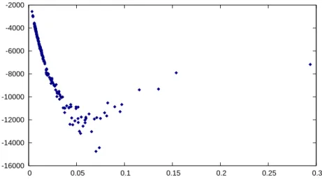
-16000 -14000 -12000 -10000 -8000 -6000 -4000 -2000 0 0.05 0.1 0.15 0.2 0.25 0.3
Figure 1:
Single name delta sensitivities of the sample bespoke CDO in Section 6 to a change of 0.10% in the CDS spread of each entity, plotted against the entity’s 5 year CDS spread (xaxis). The calcula-tion is based on data from 22 January 2009.Let’s now see how this algorithm can be adapted to the stochastic re-covery case. In the deterministic rere-covery case, the loss given default in equation (22) is given by
LGDj :=wj(1−Rj) (24)
wherewj is the corresponding weight in the portfolio andRjis the recovery
rate of entity j. In general, stochastic recovery translates into stochastic loss given default, therefore instead of a uniqued(i), we would end up with a range of possible target buckets. However, we can take advantage of the particular stochastic recovery specification described in Section 4: if recovery is a deterministic function of the copula factor as in (15), then it becomes deterministic once we set the factor equal to a fixed valuez for our conditional calculations. Loss given default is thus given by
LGDj :=wj(1−Rj(z)) (25)
whereRj(·) is the recovery rate function defined in equation (15).
To demonstrate a practical application of the algorithm, in Figure 1 we chart single name delta sensitivities for the bespoke CDO that we will use later on in Section 6 for our step-by-step mapping example. The single name deltas are obtained with a fast delta algorithm that calculates each sensitivity by removing the relevant entity from the portfolio loss distribu-tion and inserting it again with a shifted default probability as suggested in [3]. As Andersen et al point out, fast sensitivity algorithms represent a practical advantage of the recursion-based framework with respect to competing approaches (such as the Fast Fourier Transform).
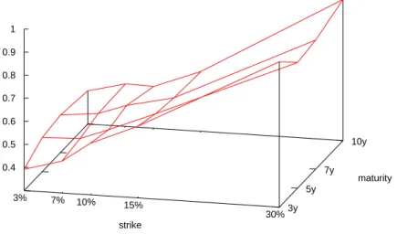
3y 5y 7y 10y 3% 7% 10% 15% 30% 0.4 0.5 0.6 0.7 0.8 0.9 1 maturity strike
Figure 2:
Base correlation surface for CDX IG Series 11 on 8 January 2009 obtained using the stochastic recovery model.4.2
Time and strike dimensions
One of the main limitations of the copula approach is that it only models the terminal distribution at a given time horizon and therefore it cannot be used consistently to introduce a dynamics for the underlying risks. To address this problem, in line with market practice we parameterize the factor copula in (13) with a single scalar parameter ρ, ie ρi = ρ ∀i. We
make ρ a function of time and strike and we calibrate its value to the price of market tradable instruments. In other words, we assume that for a given time horizonT and a given base tranche detachmentd, the terminal loss distribution can be constructed by imposing a flat pairwise correlation
ρ(d, T) among default indicators in the underlying pool. We callρ(d, T) the ‘correlation surface’ (see Figure 2 for an example), while for a fixed time horizon ¯T, we call the curve ρ(d,T¯) the ‘correlation skew’ for maturity
¯
T. The points on the correlation surface are obtained by reproducing the market prices of standard tranches, so it is normally possible for instance to build a correlation surfaceρEUs(d, T) for the iTraxx Europe index and
a correlation surfaceρNAs(d, T) for the CDX NA IG index, wheresis the
relevant index series. At the time of writing this paper, in a context of general illiquidity an active market was also available in other tranched indices, namely the CDX NA High Yield index and the LCDX index.
Before moving on to mapping methods, it’s important to clarify how the time and strike dimensions of the correlation surface impact the pric-ing of base tranches. The discounted payoff of the legs of a base tranche
in equations (9) and (10) depends on the loss distribution at all times be-tween time 0 and the maturity of the tranche. A common approximation consists in discretizing the leg payoffs at quarterly intervals in coincidence with the premium payment dates [16]. In order to preserve consistency, for the pricing of a base tranche we use the full term structure of (time dependent) correlations for a given detachment point from the time origin to the maturity of the deal. For example, we use the 5 year correlation at 6% detachment ρEU10(0.06,5) to build the loss distribution at the 5 year point in time for all three iTraxx Europe Series 10 standard base tranches detaching at 6%: with 5 year, 7 year and 10 year maturity. In contrast, for each time horizon only one point of the correlation skew is involved in the calculation of a base tranche cash flows: the correlation associated with the base tranche detachment point.
A corollary of the time dependent parameter structure is that extrapo-lation assumptions that extend the correextrapo-lation surface from the first avail-able tranche maturity backwards to the time origin have an impact on the pricing of the tranches in strike-interpolation region as well. For instance, given that the shortest available standard tranche maturity for the iTraxx Europe Seriessis 5 years, a common practice in the market is to build the relevant correlation surface on the assumption that
ρEUs(d, t) :=ρEUs(d,5) t <5 (26) for any detachment pointd, wheret is measured in years. In general this practice may lead to inconsistent expected loss surfaces (see also Section 4.3 for a discussion of consistency criteria). Time-extrapolation below the shortest available standard tranche maturity is better performed in the base expected loss space as in [16]. See also our comments in Section 5.4 on the possibility of using older series of an index to refine the maturity grid of the correlation surface.
We conclude this section by observing that one does not need any in-terpolation or extrapolation assumptions in the strike dimension when cal-ibrating the correlation surface to the market prices of standard tranches. In contrast, interpolation and extrapolation in the time dimension are nec-essary to produce quarterly loss distributions for the pricing of the standard base tranche legs.
4.3
Pillars and surface
Each point on the correlation surface provides a full specification of the factor copula parameter for a given time horizon. In other words, our port-folio loss model is non-prescriptive about how to join two points (or pillars) on the correlation surface. For indices, the surface is built from a set of pil-lars in correspondence of the liquid standard tranche detachment/maturity pairs (normally 15 for the iTraxx and 20 for the CDX as the 3 year matu-rity is also available1 ). One of the issues when evaluating non-standard
1In 2006 some major tranche dealers tried to develop a market for standard tranchelets
(index tranches with 1% thickness) and in particular for the 0-1%, the 1%-2% and the 2%-3% tranchelets, with the aim of improving price transparency and the resolution of the correlation
tranches is therefore how to extend the pillar information set to obtain the surface via interpolation or extrapolation of the skew as appropriate.
In the context of the base correlation surface setting, we can argue that a similar class of problems is the construction of volatility surfaces for op-tions on other underlying assets. For foreign exchange opop-tions for instance the Vanna-Volga approach [6] provides a consistent empirical procedure to construct implied volatility curves based on static replication and hedging arguments. In this regard, by striking a parallel with volatility surfaces we want to highlight a profound difference with the construction of correlation surfaces. Due to the incomplete-maket nature of the CDO pricing prob-lem, the hedging of a bespoke tranche using tranched exposure on different underlying portfolios necessarily leaves some open risk [17]. The only ar-bitrage constraints that one can impose are based on the requirement to build a consistent loss distribution for a given portfolio. In [11] Greenberg identifies two criteria of possible inconsistency:
BEL(d1, T)<BEL(d2, T) ford1≥d2 (capital structure inconsistency)
BEL(d, T1)<BEL(d, T2) forT1≥T2 (maturity inconsistency)
where Base Expected Loss BEL(d, T) is the expected value of terminal base tranche loss (6) at maturityT:
BEL(d, T) :=E[Ld(T)] (27)
These consistency conditions can be used to determine a range of no-arbitrage prices for non-standard tranches where a set of standard tranches exists for the underlying pool, as is the case for liquid CDS indices.
By looking at the problem in the base expected loss space, Parcell and Wood for instance [20] find that the correlation skew may turn to a smile below 3% attachment point. This finds supporting evidence in the shape of the 3-7% CDX skew, which has taken negative values starting from the last months of 2008 (see Figure 6 for an example). Looking at arbitrage costraints in the expected loss space has the advantage that the problem is always formulated as an interpolation problem and never as an extrap-olation one. However, the mapping methodology as we know it and as it will be detailed in the following sections is based on correlation surfaces. Therefore, although we are currently working on the definition of a map-ping methodology based on expected loss surfaces, for this paper we will stick to the correlation surface setting.
In this respect, the problem of extrapolating correlation skews below 3% attachment is a particularly sensitive issue. In the course of 2008, the considerable number of high profile credit events and low realized recoveries resulted in high incurred default loss in the underlying pool of many single tranche CDO deals in the market. As a consequence, these deals saw their subordination eroded. In some cases the attachment point of once AAA rated mezzanine deals became so low that they started mapping to extrap-olation region below 3% attachment point (or equivalent lowest abscissa in the mapping skew domain, see Section 5.2).
surface in the equity part of the capital structure [9]. These attemps appear to have been abandoned. See Section 3.2 of [5] for a sample calibration of the dynamical Generalized-Poisson Loss process to tranchelet prices on 1st March 2006.
The problem of building a consistent correlation surface from the pillars associated with a set of standard tranches is still elusive and possibly may not have a solution in the gaussian factor modelling framework.
5
Mapping
The exercise of inferring appropriate dependence parameter values for the pricing of bespokes from the market prices of standard tranches takes the name of ‘mapping’ [4] 2 . In a nutshell, mapping consists in adapting to
bespoke pools the dependence structure of CDS index pools. The method-ology is based on finding ‘equivalent strikes’: given two poolsP1 and P2,
the strikesd1 andd2 of two base tranches BP1(d1, T) andBP2(d2, T) are
said to have equivalent strikes if
M(BP1(d1, T)) =M(BP2(d2, T)) (28)
whereM is a real-valued function called ‘mapping method’. A key property of mapping methods is that they must be strictly monotonic functions of strike for a fixed maturity. In other words, for a given portfolioP if we fix
T then
d1> d2 ⇒ M(BP(d1, T))> M(BP(d2, T)) (29)
Mapping methods are in general a function of all the parameters of the portfolio loss model. For our mapping exercise we preserve the base tranche framework, this means that in order to map a single tranche CDO, both its attachment and detachment base tranches have to be separately mapped.
5.1
A list of alternative mapping methods
In this section we define some popular mapping methods. We first intro-duce some useful quantities or expected values that will be used for the definitions (all expectations will be taken at time 0).
We have already defined Base Expected Loss (27) in Section 4.3. Base Expected Discounted Loss BEDL(d, T), which is also sometimes referred to in the literature as ‘base expected loss’ [20], is the expected value of discounted base tranche loss. Equivalently, it is equal to the expected value of the protection leg of a base tranche (9) with detachment d and maturityT: BEDL(d, T) :=E " Z T 0 D(0, t)dLd(t) # =E[BaseProtection(d, T)] (30)
The two quantities just introduced are also defined for the underlying pool (or equivalently for the base tranche detaching at 100%) and take the names of Expected Pool Loss
EPL(d, T) := BEL(1, T) (31)
2 It came with a slight irony that the dealer which provided the most widely used reference
paper on mapping unwittingly forced many investors to think again about the value of their CDO exposure by falling a victim to the credit crisis on 15 September 2008.
and Expected Pool Discounted Loss
EPDL(d, T) := BEDL(1, T) (32) These two quantities are clearly not a function of the dependence structure imposed onP as they are equal to the sum of expected (discounted) losses on a linear basket of single name CDS contracts on the pool constituents.
At the time of writing this paper, among the mapping methods most widely used in the market (see [4] and [10]) were:
• No mapping (‘NM’)
MNM(BP(d, T)) :=d (33)
• At-The-Money (‘ATM’)mapping
MATM(BP(d, T)) := d
EPL(T) (34)
• Tranche Loss Proportion (‘TLP’)mapping
MTLP(BP(d, T)) :=
BEL(d, T)
EPL(T) (35)
• Tranche Discounted Loss Proportion (‘TDLP’)mapping
MTDLP(BP(d, T)) :=
BEDL(d, T)
EPDL(T) (36)
• Probability Matching (‘PM’)mapping
MPM(BP(d, T)) :=P[LP(T)≤d] (37)
An exhaustive comparative analysis of alternative mapping methods is be-yond the scope of this paper; we’re more interested in detailing the mod-elling framework and in highlighting potential pitfalls with the methodol-ogy. We refer to Section 5.5 for some considerations regarding the alterna-tive mapping functions.
5.2
Mapping surface
In Figure 3 we chart the points (M(BEU10(d, T), ρ), ρ) for all the standard
detachment pointsdof the iTraxx Europe Series 10 index withT equal to the five years maturity using three different mapping methods: NM, TDLP and PM. Thoughout the paper we’ll refer to this type of chart as a ‘mapping skew’. The mapping skews in Figure 3 clarify along what lines the mapping operates: the strike domain of the correlation skew is rearranged based on the mapping method, so that data points corresponding to the standard base tranches are effectively only moved horizontally in the plot.
The NM skew is actually equal to the correlation skew of the index as defined in Section 4.2. In the PM mapping skew, the correlation skew is transformed by mapping detachment points to quantiles of the portfolio
0 0.2 0.4 0.6 0.8 1 0 0.2 0.4 0.6 0.8 1 5y No Mapping 5y Tranche Discounted Loss Proportion 5y Probability Matching
Figure 3:
Mapping skew of iTraxx Europe Series 10 5y standard tranches for 6 January 2009 for the NM method, the TDLP method and the PM method.loss distributions. The structure of correlation parameters in our modelling approach further introduces a maturity dimension to the mapping skew in a natural way, so that we can talk about the ‘mapping surface’ of a particular portfolio. We can therefore introduce analogous notation to correlation surfaces where the detachment point variable is replaced by its image in the chosen mapping space. By way of example, the mapping surface for the PM mapping surface of iTraxx Europe Seriess index will be denoted
ρEUPMs(x, T).
The whole point about mapping is that one assumes that the mapping surface obtained from market prices of liquid index tranches can be applied by analogy to a bespoke portfolio. The mapping surface can then be used to back out a correlation surface for the bespoke pool, as the strike space is the most convenient for evaluation purposes in a base tranche setting. The process can be represented schematically as follows:
index tranche prices (→a) index corr surface (→b) index mapping surface
(c)
=:
bespoke tranche price (←e) bespoke corr surface (←d) bespoke mapping surface
base correlation surface ρI for index I is obtained by calibrating to the
market prices of standard tranches. In step (b) strikes are mapped using the method of choice:
(d, T)7→(M(BI(d, T)), T) (38)
where BI denotes index base tranches. If we fix maturity T and define fTI(d) = M(BI(d, T)) then the increasing property (29) implies that the
inverse function (fTI)−1 exists. Therefore the mapping surfaceρIM can be written in terms of the correlation surface:
ρIM(x, T) =ρ I
((fTI)−
1
(x), T) (39)
In step (c) the bespoke mapping surfaceρ∗
M is set equal to the index
map-ping surface
ρ∗M(x, T) :=ρIM(x, T) (40) Let’s denote with B∗ the base tranches of the bespoke pool and define fT∗(d) =M(B∗(d, T)) in an analogous fashion as in step (b). The bespoke
correlation surface is obtained from the bespoke mapping surface in step (d)
ρ∗((fT∗)−1(x), T) =ρ∗M(x, T) (41) If the index correlation surface is defined on a set {dI} of surface pillars
equal to the set of standard tranche detachment points, then the bespoke correlation surface is defined on a set of transformed pillars{d∗}, where for each detachment/maturity pair (dI, T)
d∗= (fT∗)−
1
(fTI(d I
)) (42)
Finally, in step (e) the bespoke correlation surface is interpolated to obtain the relevant term structures of correlations for the pricing of attachment and detachment base bespoke tranches.
5.3
Limits of correlation mapping
One of the first tests that are normally performed when discussing the rel-ative merits of different mapping methods is the mapping of iTraxx Europe tranches onto CDX tranches. The reasoning behind this is that correla-tion mapping consists in defining “market invariants” [10] that should be used for the pricing of tranched exposures. Usually these tests do not give encouraging results, showing if anything that the market uses different cor-relation assumptions for pricing the loss distribution of the two most liquid sets of standard tranches. Figure 4 shows for instance the PM mapping skew for both CDX and iTraxx on 10 November 2008: possibly reflect-ing the perception of a higher systemic risk component, it is evident that market is pricing in a higher correlation for loss quantiles in the North American pool.
We take a different view on the meaning of mapping, in that we believe that the two following considerations define a more transparent conceptual framework for the application of mapping methods:
0 0.2 0.4 0.6 0.8 1 0 0.2 0.4 0.6 0.8 1 5y iTraxx 5y CDX
Figure 4:
PM Mapping skew of 5y iTraxx Europe Series 10 and 5y CDX NA IG Series 11 on 10 November 2008.1. Rather than possible market invariants, we think that mapping meth-ods should represent possible ways of using all available market infor-mation on credit correlation for the pricing of non-standard tranched exposures. In other words, with mapping we’re looking for a way of analyzing the (scarce) market information on credit correlation and of incorporating it into our pricing problem.
2. In addition, and possibly more importantly, one should always keep in mind that the estimation of a price for an unmarketed CDO is an incomplete-market problem and that there is normally a broad range of prices that are consistent with no-arbitrage constraints. Neverthe-less, as pointed out by Walker [24], for reporting purposes practition-ers need a well-defined procedure for determining a definite estimate of the value of their CDO positions. This procedure will generally reflect the practitioner’s preferences with respect to the risk and re-turn of the relevant exposures. We consider mapping methods as a means of expressing our preferences via the definition of an acceptable evaluation procedure for bespoke CDOs.
Along the lines of the first consideration, the set of CDX tranche prices and the set of iTraxx tranche prices both represent complementary market information and should both be used for the mapping exercise. It is still possible that at some point in time a part the correlation skew for both liquid indices can be explained by the same ‘invariant’ transformation of -say - the distribution of single name CDS spreads in its underlying pool.
0 0.2 0.4 0.6 0.8 1 0 0.2 0.4 0.6 0.8 1 Series 9 Series 10
Figure 5:
PM mapping skew of 5y iTraxx Europe Series 9 and Series 10 on 12 November 2008.However, considering how scarce liquid tranche price information is and how different the European and North American credit markets are, it would be rather surprising if we were able to further reduce the rank of the correlation data set by mapping the two most liquid correlation surfaces onto each other.
5.4
A closer look at the data
We have seen in the previous section that different sets of correlation in-formation are normally associated with CDX and iTraxx indices. On the other hand, if we look at successive series of an individual credit index, we expect to find evidence of consistency of pricing assumptions in the market. After all, adjacent series of an index differ normally only by a handful of names. In Figure 5 we show the PM mapping skew for 5y iTraxx Europe Series 9 and Series 10 on 12 November 2008. The underlying pools of the two series differ by 6 entities on a total of 125. Despite the 6 month dif-ference in the maturity between the two index series, we observe that the relevant mapping skews were almost coincident on that particular day.
If we assume that different series of an index have very similar corre-lation data structures, we may even try to enlarge the data set for our calibration by including data from different series of the same index in or-der to obtain a finer maturity grid. In Figures 6 and 7 we show some data that seems to support this proposition. In both figures the skews have been calibrated separately for each index series. It is again quite evident that
0 0.2 0.4 0.6 0.8 1 0 0.2 0.4 0.6 0.8 1 IG S11 Dec-2011 IG S9 Dec-2012 IG S11 Dec-2013 IG S9 Dec-2014
Figure 6:
PM mapping skew for select maturities of CDX NA IG Series 9 and Series 11 on 22 January 2009.0 0.2 0.4 0.6 0.8 1 0 0.2 0.4 0.6 0.8 1 ITX S8 Dec-2012 ITX S10 Dec-2013 ITX S8 Dec-2014 ITX S10 Dec-2015
Figure 7:
PM mapping skew for select maturities of iTraxx Europe Series 8 and Series 10 on 22 January 2009.the correlation structure associated with the CDX index is quite different from the one associated with the iTraxx index.
5.5
Choice of mapping method
We refer to [4] for a list of desirable properties of mapping methods and for a discussion of the relative merits of alternative methods, with particular reference to ATM, PM and TLP.
As we’ve seen in Section 5.2, mapping methods only rearrange corre-lation surface pillars in a transformed domain. In this respect, an addi-tional desirable feature is that the mapping method of choice should avoid producing steep mapping skews. A steep skew increases the impact of in-terpolation assumptions and amplifies potential numerical noise together with the sensitivity of mapped correlation to a change in attachment point. In fact, producing a flat skew is generally a desirable property of credit correlation models, because a steep correlation skew may result in the pric-ing of mezzanine tranches uspric-ing very different parametric assumptions for the loss distribution at attachment and at detachment. Valuing different parts of the same payoffs with different model parameters may lead to in-consistencies and potentially to negative expected tranche loss as pointed out in [22]. We observe that if a model were able to produce a flat skew, then all mapping methods would produce the same result and would all be equivalent to applying the NM method.
In [4] the authors conclude that both the TLP and PM methods give reasonable results and are superior to ATM. Based on evidence available to them, TLP performed better than PM in some instances, such as mapping iTraxx Europe Series 6 to CDX NA IG Series 7. However, they mention that PM is the only method among the three that is continuous with respect to expected default events,ieto changes in the value of a tranche due to a name with a very high default probability actually defaulting (see discussion on “Value on Default” in [4] p. 11). In our experience the TLP method produces steeper and less stable skews with respect to PM. We note that a possible drawback of the PM method from the point of view of Baheti and Morgan might have beed represented by a potential issue with unstable risk parameters due to the fact that with deterministic recovery the loss distribution is discrete ([4] p. 6).
Overall, among the mapping methods that we tested, we favour PM mapping due to several considerations, including:
• it has a straightforward interpretation in terms of mapping quantiles of the terminal loss distribution;
• by producing a smooth loss distribution, the introduction of stochastic recovery specifications solves the issue with unstable risk parameters; • the method generally produces relatively flat and stable mapping
skews;
• it is continuous with respect to expected default events.
In any case, in order to reduce model risk, most practitioners calcu-late a range of bespoke tranche valuations by applying correlation surfaces
obtained using different mapping methods, if not different portfolio loss models.
6
A step-by-step example
In the previous sections we have detailed the modelling approach for con-structing the loss distribution in the underlying pool, we have defined a conceptual framework for mapping and we have discussed some related is-sues. We are now going to see how all the pieces fit together by reviewing step by step a possible evaluation process for a sample bespoke CDO. This will allow us to clarify our preferred valuation procedure and to identify potential weaknesses associated with it.
Let’s consider a CDO with a maturity T∗ of 20 December 2014 and a diversified underlying pool of 180 equally weighted investment grade names composed for 40% of European entities, for 50% of North American entities and for the remaining 10% of Asian and Australian entities. Attachment point isa∗= 2.25% and detachment point isd∗= 5.25%. Base tranches on our bespoke pool with detachment pointdand maturityT will be denoted
B∗(d, T).
Step 1. Select the mapping domain
The first step consists in choosing appropriate market correlation surfaces to map the deal to. This step already involves some discrimination in selecting the relevant market information set. For our sample deal we are clearly looking at the iTraxx and CDX correlation surfaces; however we can make here two considerations: the first is that these two sets of tranches are not the only ones that are traded in the market. For deals where the underlying pool is composed of speculative grade issuers for instance, including the CDX NA High Yield tranches in the information set may be more appropriate; LCDX tranches may also be used for the mapping of Collateralized Loan Obligations.
The second consideration is that one may assume that the latest series of an index, besides being the most liquid in the index CDS market, also constitutes the underlying pool of the most liquid set of standard tranches. However, at the time of writing this paper, standard tranches on Series 9 of both the iTraxx and CDX were more liquid than on the respective on-the-run index series (namely, iTraxx Europe Series 10 and CDX NA IG Series 11). This could be explained with the fact that the bulk of existing CDO exposure in the market was executed when iTraxx or CDX Series 9 was the on-the-run index. For this reason, Series 9 iTraxx and CDX tranches are still the most used in the market for hedging purposes, as in many cases they provide a better match for a seasoned bespoke deal in terms of maturity and underlying pool composition. In conclusion, one should select the standard tranches to be used as an input information set for the mapping problem by taking into account not only how well the bespoke pool can be represented by index constituents, but also what series of the index is the most liquid and best matches the characteristics of the bespoke tranche.
Step 2. Build implied correlation surfaces for the
rele-vant indices
Let’s assume that we have determined that the relevant indices in the map-ping domain for our sample bespoke are the iTraxx Europe Series 10 and the CDX NA IG Series 11. As a next step we calibrate the correlation pa-rameter in correspondence of standard tranche pillars for the two indices. We further assume that we have devised an appropriate method for build-ing the correlation surfacesρEU10andρNA11from the relevant set of pillars
(see considerations in Section 4.3), so that the two surfaces are defined for all strike/maturity pairs.
We observe that, given the value ofa∗, the lower strike of our bespoke tranche will likely map to extrapolation region below 3% attachment of the two indices.
Step 3. Apply mapping method of choice to each set of
standard tranches
Let’s assume that we have established that the market information set for evaluating our bespoke tranche should be composed of the current on-the-run standard tranches for iTraxx and CDX. The next step is apply our mapping method(s) of choice to obtain attachment and detachment base correlations for the bespoke deal. We further assume that our preferred mapping method is the Probability Matching method.
First of all we observe that the bespoke tranche can be mapped to only one tranched index at a time. Considering that we have two indices in our mapping domain, by applying the mapping we will obtain two correlation surfaces ρ∗(EU10) and ρ∗(NA11). Both correlation surfaces are obtained as
outlined in Section 5.2. For instance, for the correlation surface obtained by mapping to the iTraxx index, the process can be represented with the following diagram:
ρEU10 → ρEU10PM
=:
ρ∗(EU10) ← ρ∗PM(EU10)
While the set of base detachment points for each index correlation surface is defined by the relevant set of available liquid standard tranches, it is up to us to choose appropriate pillars for correlation surfacesρ∗(EU10) and
ρ∗(NA11). In terms of strikes, for our valuation problem we’re only inter-ested in two detachment points, namely a∗ and b∗. However, based on
the considerations we made in Section 4.2, a slightly different approach is required for choosing the relevant pillars in the time dimension.
Let’s take the CDX NA IG index to clarify this point. CDX standard maturities in years are{3,5,7,10}, while our bespoke tranche has a maturity of 6 years. Because we’re working with time-dependent correlations, we always need the full term structure up to the maturity of the tranche to be priced. Therefore we choose {3,5,7} as maturity pillars on ρ∗(NA11),
where we have included the 7 year maturity as it is needed to interpolate to 6 years, while we have excluded the 10 year maturity because it is not required for interpolation purposes.
Step 4.
Blend mapped correlation surfaces based on
index weights
At the end of step 3 we were left with the following relevant pillars on the mapped correlation surfaces for our sample deal:
ρ∗(EU10)(2.25%,5) ρ∗(EU10)(2.25%,7)
ρ∗(EU10)(5.25%,5) ρ∗(EU10)(5.25%,7)
ρ∗(NA11)(2.25%,3) ρ∗(NA11)(2.25%,5) ρ∗(NA11)(2.25%,7)
ρ∗(NA11)(2.25%,3) ρ∗(NA11)(5.25%,5) ρ∗(NA11)(5.25%,7)
We now have to blend these values to arrive at a single correlation set for our bespoke tranche valuation exercise. At the time of writing this paper, prevailing market practice was to assign a weight to surfaceρ∗(EU10)equal
to the aggregate weight wEU of European names in the underlying pool,
while surfaceρ∗(NA11) was assigned a weight of (1−w
EU). In particular,
for our example we can write:
ρ∗(d, T) =wEUρ∗(EU10)(d, T) + (1−wEU)ρ∗(NA11)(d, T) (43)
where wEU = 40% and ρ∗(EU10)(d,3) = ρ∗(EU10)(d,5). Although possibly
the rationale for allocating all non-European entities to the weight of the North American index was originally motivated with considerations regard-ing the composition and spread distribution of the relevant entities, it is evident that this is one of several steps in the mapping process where a degree of judgement is involved.
Step 5. Compute value of bespoke tranche
With the correlation values obtained in the previous step we can build a term structure of base correlations and price attachment and detachment base tranches of our bespoke deal.
We conclude the section by observing that at Step 1, depending on the composition of the underlying bespoke pool and on the relative liquidity of standard tranches in the market, we might have chosen iTraxx Europe Series 8 and CDX NA IG Series 9 as the mapping domain. The 7 year ma-turity of these two indices would have matched the mama-turity of the bespoke deal.
7
Diversification and skew adjustments
Risk managers may take the view that adapting index correlation surfaces to bespoke pools via mapping represents an addition source of model risk. Specific reserves may be set aside to provide a cushion against uncertainty in the determination of the correlation parameters.
The value of thin tranches,ietranches where the difference between de-tachment and atde-tachment strike is low (usually below 3% for high grade), is
particularly sensitive to the mapped skew, which is the difference between mapped detachment base correlation and mapped attachment base corre-lation. Especially in the case of bespoke tranches that are junior enough to map into extrapolation region, reserves may be added by conservatively applying a flat skew.
Another adjustment to mapped correlations is based on the consider-ation that a bespoke portfolio like the one that we used in the previous section appears to be more diversified than the individual indices, both geographically and in terms of the relative weight of each entity. A higher level of diversification is generally associated with a lower level of corre-lation, therefore index skews in the mapping domain should not only be rearranged horizontally (see Section 5.2), but they should also be shifted vertically by applying diversification haircuts to the mapped correlations. The haircuts, which (where applicable) are meant to account for higher diversification in the bespoke pool compared to individual indices, should be determined where possible by calibrating to prices of bespoke tranches available in the market.
Along the same lines, if a bespoke pool is less diversified than an in-dex in its mapping domain (consider for instance a portfolio limited to a few corporate sectors), then a risk manager may consider calculating re-serves based on adjusting mapped correlation upwards. Again, judgement is clearly involved together with all expedients of prudent risk management.
8
Conclusion
In this document we discuss a popular methodology for the pricing of sin-gle tranche CDOs in a recently proposed stochastic recovery setting. We highlight key assumptions and identify possible pitfalls. Areas of further investigation include consistent construction of correlation surfaces, the def-inition of a mapping methodology based on expected loss and research on mapping in a dynamic credit modelling framework.
The extreme market conditions that the credit markets in particular have experienced in 2008 provide invaluable insight for the advancement of the relatively young theory of credit correlation. We believe that the ratio-nale for a market in the loss distribution of portfolios of credit exposures remains solid. At the very least, CDO products helped to expose and cor-rect a flawed market consensus on the nature of multivariate default risk, in particular when associated with leverage. Part of the challenge is tech-nological and is connected to the complexity of the risks associated with CDO transactions and to the sheer amount of information to be managed and analysed.
References
[1] Amraoui S. and Hitier S., “Optimal Stochastic Recovery for Base Cor-relations”,BNP Paribas, June 2008.
[2] Andersen L. and Sidenius J., “Extensions to the Gaussian Copula: Random Recovery and Random Factor Loadings”, Bank of America, June 2004.
[3] Andersen L., Sidenius J. and Basu S., “All your hedges in one basket”, Risk November 2003, 67-72.
[4] Baheti P. and Morgan S., “Base Correlation Mapping”,Lehman Broth-ers Quantitative Credit Research Quarterly, March 2007.
[5] Brigo D., Pallavicini A. and Torresetti R., “Calibration of CDO Tranches with the Dynamical Generalized-Poisson Loss Model”, Banca IMI, May 2007.
[6] Castagna A. and Mercurio F., “The Vanna-Volga Method for Implied Volatilities”, Risk January 2007, 106-111.
[7] www.creditfixings.com/information/affiliations/fixings/auctions/2008.shtml [8] www.creditflux.com/resources/index+tranches.htm
[9] “Credit Houses Make Inroads Into Tranchelets Market”, Derivatives Week, 23 January 2006.
[10] Garcia J. and Goossens S., “Correlation Mapping Under L´evy and Gaussian Base Correlation”, Dexia Group, September 2008.
[11] Greenberg A., “Arbitrage-Free Loss Surface Closest to Base Correla-tions”, Rabobank International, July 2008.
[12] Gregory J., “A Decade of CDO Pricing”, Slides for the World Congress on Computational Finance, March 2007, available at http://www.riskwhoswho.com/Resources/GregoryJon1.ppt#2 [13] Hull J. and White A., “Valuation of a CDO and an nth to Default
CDS Without Monte Carlo Simulation”, Joseph L. Rotman School of Management, University of Toronto, September 2004.
[14] Hull J. and White A., “An improved implied copula model and its application to the valuation of bespoke CDO tranches”, Joseph L. Rotman School of Management, University of Toronto, April 2008. [15] Krekel M., “Pricing distressed CDOs with Base Correlation and
Stochastic Recovery”, UniCredit Markets & Investment Banking, May 2008.
[16] Krekel M. and Partenheimer J., “The Implied Loss Surface of CDOs”, December 2006.
[17] Laurent J.-P., “A note on the risk management of CDOs”, ISFA Ac-tuarial School & BNP Paribas, February 2007.
[18] Laurent J.-P. and Gregory, J., “Basket Default Swaps, CDO’s and Factor Copulas”, September 2003.
[19] Morini M. and Brigo D., “Arbitrage-free pricing of Credit Index Op-tions. The no-armageddon pricing measure and the role of correlation after the subprime crisis”, December 2007.
[20] Parcell E. and Wood J., “Wiping the smile off your base (correlation curve)”, Derivative Fitch, June 2007.
[21] Scheicher M., “How has CDO market pricing changed during the tur-moil? Evidence from CDS index tranches”, European Central Bank, Working Paper Series No. 910 / June 2008.
[22] Torresetti R., Brigo D. and Pallavicini A., “Implied correlation in CDO tranches: a paradigm to be handled with care”, Banca IMI, November 2006.
[23] Torresetti R., Brigo D. and Pallavicini A., “Implied Expected Tranched Loss Surface from CDO Data”, Banca IMI, May 2007. [24] Walker M. B., “An Incomplete-Market Model for Collateralized Debt