Forecasting monthly airline passenger numbers with small datasets using feature engineering and a modified principal component analysis

(1)

Forecasting Monthly Airline Passenger

Numbers with Small Datasets Using

Feature Engineering and a Modified

Principal Component Analysis

Sara Al-Ruzaiqi

A Doctoral Thesis

Submitted in partial fulfilment

of the requirements for the award of

Doctor of Philosophy

of

(2)

2019

Dedication

I dedicate this Thesis to the two most important people in my life my father and my mother (my beloved parents) for their endless support and unconditional love. My parents always believed in me even in times when I was full of doubt in myself. They were always there cheering me up and stood by me through the good and bad times.

(3)

Abstract

In this study, a machine learning approach based on time series models, different feature engineering, feature extraction, and feature derivation is proposed to improve air passenger forecasting. Different types of datasets were created to extract new features from the core data. An experiment was undertaken with artificial neural networks to test the performance of neurons in the hidden layer, to optimise the dimensions of all layers and to obtain an optimal choice of connection weights – thus the nonlinear optimisation problem could be solved directly. A method of tuning deep learning models using H2O (which is a feature-rich, open source machine learning platform known for its R and Spark integration and its ease of use) is also proposed, where the trained network model is built from samples of selected features from the dataset in order to ensure diversity of the samples and to improve training. A successful application of deep learning requires setting numerous parameters in order to achieve greater model accuracy. The number of hidden layers and the number of neurons, are key parameters in each layer of such a network. Hyper-parameter, grid search, and random hyper-parameter approaches aid in setting these important parameters. Moreover, a new ensemble strategy is suggested that shows potential to optimise parameter settings and hence save more computational resources throughout the tuning process of the models. The main objective, besides improving the performance metric, is to obtain a distribution on some hold-out datasets that resemble the original distribution of the training data. Particular attention is focused on creating a modified version of Principal Component Analysis (PCA) using a different correlation matrix – obtained by a different correlation coefficient based on kinetic energy to derive new features. The data were collected from several airline datasets to build a deep prediction model for forecasting airline passenger numbers. Preliminary experiments show that fine-tuning provides an efficient approach for tuning the ultimate number of hidden layers and the number of neurons in each layer when compared with the grid search method. Similarly, the results show that the modified version of PCA is more effective in data dimension reduction, classes reparability, and classification accuracy than using traditional PCA.

Keywords: Feature Engineering; Deep Learning; Principle Component Analysis (PCA); algorithm; prediction.

(4)

Acknowledgements

First of all, I would like to address my most precious appreciation to my supervisor Dr Christian Dawson for his guidance and encouragement through this work. His profound knowledge, positive attitude, patient guidance, and valuable suggestions on my work guaranteed the completion of this Thesis. One simply could not wish for a better or friendlier supervisor. He has set an example of excellence as an instructor and a mentor. I have been extremely lucky to have a supervisor who cared so much about my work. My special acknowledgements go to all those people who provide me with data for my experiments. My warm appreciation is due to the Public Authority for Civil Aviation, Directorate General of Meteorology, and Ministry of Tourism in Oman.

My warmly acknowledge go to his majesty Sultan Qaboos government the Ministry of Higher Education (my sponsor) and Cultural Attaché (Embassy of Oman) for providing the financial assistance and support throughout the research period.

I cannot find proper words to express my deep gratitude to my family and friends for their sincere encouragement and inspiration during this period, which helped to bring me into this stage of my life.

And, last but not least, I would like to thank all who have knowingly and unknowingly helped me and been involved in the successful completion of this report.

Sara Al-Ruzaiqi

Loughborough, England 20.09.2019

(5)

Abbreviations

ACF Auto correlation function

GDP Gross Domestic Product

ANN Artificial neural network model

AR Autoregressive models

ARIMA Autoregressive Integrated Moving Average

ARIMAX Auto Regressive Integrated Moving Average with Exogenous Input

BSM Basic Structural models

CRM Customer relationship management

DGP Data generating process

H2O Open source machine learning platform

MA Moving Average models

MAD Mean Absolute Deviation

MAE Mean Absolute Error

MAPD Mean Absolute Percentage Error

MAPE Mean Absolute Percentage Division

MASE Mean Absolute Scaled Square Error

MECA Ministry of Environmental and Climate Affairs

MSA Mean Absolute Error

MSE Mean Square Error

MSPE Mean Squared Prediction Error

PCA Principal Component Analysis

PACF partial auto correlation function

RAE Relative Absolute Error

RMSE Root Mean Squared Error

RRSE Root Relative Squared Error

SES Simple exponential smoothing

SMAPE Symmetric Absolute Percentage Error

S Seasonal component of a time series

T Trend component of a time series

(6)

yˆ Vector of time series forecasts

ω Combination weight vector

e Unity vector

ε Forecast error

yˆ Time series forecast

yˆc Combined time series forecast

ω Weights for linear forecast combination

(7)

List of Figures

FIGURE 3-1LOCATION OF OMAN’S FOUR AIRPORTS. ... 69

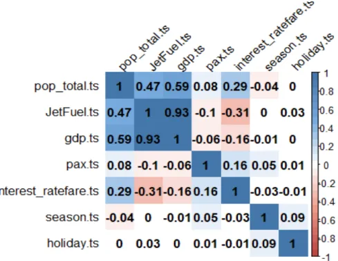
FIGURE 3-2CORRELATIONS BETWEEN TOTAL PASSENGER AND THE OTHER VARIABLES. ... 79

FIGURE 3-3MONTHLY DEPARTING PASSENGERS (IN 1000S). ... 84

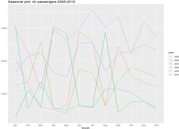
FIGURE 3-4SEASONAL PLOT:AIR PASSENGERS. ... 85

FIGURE 3-5THE TRANSFORMED DATA SERIES. ... 86

FIGURE 3-6BENCHMARK MODEL. ... 89

FIGURE 3-7MONTHLY AVERAGE BASE FARE EFFECT ON PASSENGER FLOW. ... 92

FIGURE 3-8MODEL1:ARIMA((PAX.TS.)=FARE.TS). ... 92

FIGURE 3-9JET FUEL PRICE EFFECT ON PASSENGER FLOW. ... 93

FIGURE 3-10MODEL2:ARIMA((PAX.TS.)=JETFUEL.TS). ... 93

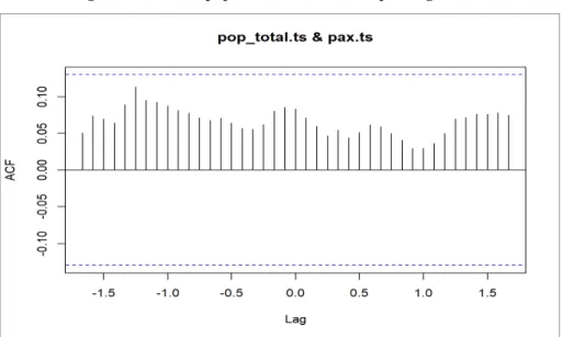
FIGURE 3-11OMAN POPULATION SIZE EFFECT ON PASSENGER FLOW. ... 95

FIGURE 3-12MODEL3:ARIMA((PAX.TS.)=POP_TOTAL.TS). ... 95

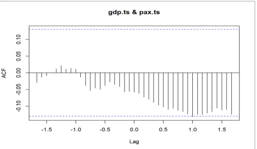
FIGURE 3-13OMAN’S GDP EFFECT ON PASSENGER FLOW. ... 96

FIGURE 3-14MODEL4:ARIMA((PAX.TS.)=GDP.TS). ... 97

FIGURE 3-15OMAN'S UNEMPLOYMENT SIZE EFFECT ON PASSENGER FLOW. ... 97

FIGURE 3-16MODEL5:ARIMA((PAX.TS.)=UNEMPLOYMENT.TS). ... 98

FIGURE 3-17OMAN’S REAL INTEREST EFFECT ON PASSENGER FLOW. ... 99

FIGURE 3-18MODEL6:ARIMA((PAX.TS.)=INTERESTRATE.TS). ... 99

FIGURE 3-19OMAN'S MONTHLY PUBLIC HOLIDAY EFFECT ON PASSENGER FLOW. ... 100

FIGURE 3-20MODEL7:ARIMA((PAX.TS.)=HOLIDAY.TS). ... 100

FIGURE 3-21THE ACTUAL MONTHLY PASSENGERS IN 2016 AND THE PREDICTIONS OF THE BENCHMARK MODEL, BENCHMARK + AVERAGE BASE FARE MODEL AND RANDOM FOREST MODEL. ... 104

FIGURE 4-1FEATURE ENGINEERING TECHNIQUES FOR AEROPLANES DATASET. ... 116

FIGURE 4-2MODEL 1:VARIABLE IMPORTANCE ON ORIGINAL FEATURES (%VAR EXPLAINED:33.43). ... 119

FIGURE 4-3MODEL2:VARIABLE IMPORTANCE WITH SEASON ON ORIGINAL FEATURES (%VAR EXPLAINED:37.13). ... 122

FIGURE 4-4MODEL3:VARIABLE IMPORTANCE WITH SEASON AND HOLIDAY ON ORIGINAL FEATURES (% VAR EXPLAINED:49.61). ... 123

FIGURE 4-5VARIABLE IMPORTANCE WITH SEASON, HOLIDAY AND GDP ON ORIGINAL FEATURES (%VAR EXPLAINED:67.06). ... 125

FIGURE 4-6VARIABLE IMPORTANCE WITH SEASON, HOLIDAY,GDP, AND JET FUEL ON ORIGINAL FEATURES (%VAR EXPLAINED:69.18). ... 127

FIGURE 4-7VARIABLE IMPORTANCE WITH SEASON, HOLIDAY,GDP, JET FUEL, POPULATION, AND INTEREST RATE ON ORIGINAL FEATURES (%VAR EXPLAINED:68.55). ... 129

FIGURE 4-8VARIABLE IMPORTANCE WITH SEASON, HOLIDAY,GDP, JET FUEL, POPULATION, INTEREST RATE, AND DISTANCE ON ORIGINAL FEATURES (%VAR EXPLAINED:67.74). ... 130

(12)

FIGURE 4-10THE ORIGINAL DISTRIBUTION OF TARGET. ... 137

FIGURE 4-11PREDICTED VALUES ON THE UNSEEN TEST SET AGAINST GROUND TRUTH-VALUES. ... 140

FIGURE 4-12THE ORIGINAL DISTRIBUTION OF TARGET. ... 141

FIGURE 4-13THE DISTRIBUTION OF PREDICTED VALUES. ... 141

FIGURE 4-14VARIABLE IMPORTANCE ON GENERATED FEATURES. ... 146

FIGURE 4-15FEATURES IMPORTANCE OBTAINED FROM DEEP LEARNING HIDDEN LAYERS. ... 147

FIGURE 5-1AIR PASSENGER NUMBERS DATA WITH PEARSON CORRELATION. ... 166

FIGURE 5-2TRAIN PASSENGER NUMBERS DATA WITH KINETIC CORRELATION. ... 166

FIGURE 5-3PRINCIPAL COMPONENT ANALYSIS FEATURES (KINETICPCA1 AND KINETICPCA2). ... 169

FIGURE 5-4FEATURES IMPORTANCE OBTAINED FROM TRAINING DATA ONLY ... 172

FIGURE 5-5FEATURES IMPORTANCE OBTAINED FROM DEEP LEARNING HIDDEN LAYERS. ... 174

FIGURE 5-6TREE-LIKE STRUCTURES OF THE GENETIC ALGORITHM. ... 177

FIGURE 5-7FEATURES IMPORTANCE OBTAINED FROM GENETIC ALGORITHM. ... 179

FIGURE 5-8FEATURES IMPORTANCE OBTAINED FROM ONE-HOT ENCODING. ... 181

(13)

List of Tables

TABLE 2-1FEATURES ARE DATE AND VISITORS; EXTRACTED FEATURE IS ISWEEKENDDAY ... 66

TABLE 3-1DOMESTIC AND INTERNATIONAL AIRPORTS IN OMAN. ... 70

TABLE 3-2POSITIVE CHANGE IN PASSENGER TRAFFIC. ... 70

TABLE 3-3EXPLORATORY DATA ANALYSIS. ... 73

TABLE 3-4ALL PROCESSED DATA. ... 75

TABLE 3-5CONSIDERATION OF MODEL AR AND/OR MA MODEL CONDITION. ... 88

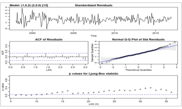
TABLE 3-6THE REGRESSION COEFFICIENT FOR ARIMA(1,0,2)X(2,0,0). ... 90

TABLE 3-7THE EVALUATION METRICS OF THE MODEL. ... 103

TABLE 4-1FEATURE MATRIX DIAGRAM.EACH ROW REPRESENTS AN EXAMPLE, AND EACH COLUMN REPRESENTS A FEATURE DESCRIBING THAT EXAMPLE. ... 109

TABLE 4-2MEMBERS TABLE FOR AIRLINE CLIENTS. ... 110

TABLE 4-3INTERACTION TABLE WITH AN E-COMMERCE AIRLINE WEBSITE. ... 111

TABLE 5-1CORRELATION MATRIX WITH THE FUNCTION O(). ... 164

TABLE 5-2CORRELATION MATRIX CORRELATION MATRIX ON BASIS OF ‘PEARSON R’ MODEL. ... 165

TABLE 5-3THE MEAN VALUES OF FEATURES OBTAINED FROM KINETIC ENERGY PCACOMPONENTS. ... 168

TABLE 5-4PREDICTION MODEL USING KINETICPCA1 AND KINETICPCA2). ... 170

TABLE 5-5THE MEAN VALUES OF FEATURES OBTAINED FROM TRAINING DATA ONLY. ... 170

TABLE 5-6PREDICTION MODEL USING TRAINING DATA ONLY. ... 172

TABLE 5-7THE MEAN VALUES OF FEATURES OBTAINED FROM DEEP LEARNING HIDDEN LAYERS. ... 174

TABLE 5-8PREDICTION MODEL USING DEEP LEARNING HIDDEN LAYERS. ... 175

TABLE 5-9THE MEAN VALUES OF FEATURES OBTAINED FROM GENETIC ALGORITHM. ... 178

TABLE 5-10PREDICTION MODEL USING GENETIC ALGORITHM. ... 179

TABLE 5-11THE MEAN VALUES OF FEATURES OBTAINED FROM ONE-HOT ENCODING. ... 180

TABLE 5-12PREDICTION MODEL USING ONE-HOT ENCODING. ... 182

TABLE 5-13THE MEAN VALUES OF FEATURES OBTAINED FROM CONDITIONAL PROBABILITY. ... 182

TABLE 5-14PREDICTION MODEL USING CONDITIONAL PROBABILITY. ... 184

TABLE 8-1FIRST FIVE ROWS OF TARGET FEATURE (PASSENGER NUMBER) ... 231

TABLE 8-2ACTUAL DATA OF NUMBER OF PASSENGERS WITH OUTLIERS 1 ... 232

(14)

(15)

Chapter 1

2.1 Introduction

Knowing the future trend of passengers travelling through air transportation is of immense importance in today’s world (Adrangi et al., 2001). It is important to ‘forecast’ the number of airline passengers as accurately as possible as such predictions can be used in many contexts ranging from simple initial planning to complicated business decisions (Carson et al., 2011). The airport facility of a country indicates the economic standard of that country (Kincaid, 2016). A global rise in overseas travel has meant that the number of passengers using airport facilities has sharply increased. In 2017, the International Air Transport Association (IATA, 2017) published their 62nd annual travel statics report based on data from its 290 airline members. IATA reports that a record number of travellers flew in 2017 between more city pairs than ever, and that a record-breaking 4.1 billion passengers flew on scheduled airline services that year. That was 280 million more than in 2016, representing a 7.3% increase year on year.

A number of different airlines operate within an airport, and to maintain a supply of facilities to meet demand accurate business and economic decisions need to be made (Tsui et al., 2011). Accurate forecasts of air transport activity are essential in the planning processes of states, airports, airlines, and other relevant bodies (Riga et al., 2009). Accurate forecasts also assist aircraft manufacturers in planning future aircraft types (in terms of size and range) and when to develop them (Cho, 2003; Cuhadar, 2014; Kulendran & Witt, 2003). Since passenger transport demand forecasting greatly affects the effectiveness of investment efficiency by adequacy and accuracy of the performance estimation, it is seen as a critical criterion for investors as well as for airlines (Market Research.com, 2017).

Air traffic forecasts are a key input into an airline's fleet planning and route network development, and are also used in the preparation of the airline's annual operating plan (Coshall, 2006). Furthermore, analysing and forecasting air travel demand may also assist an airline in reducing its risk through an objective evaluation of the demand side of the airline business (Cho, 2003; Cuhadar, 2014; Kulendran & Witt, 2003).

(16)

Identifying the potential impact of the future trend of airline passengers, this study intends to thoroughly analyse the pattern of airline passengers travelling through Muscat International Airport in Oman. The study aims to establish a prediction mechanism for future values of airline passenger numbers of this airport, which has experienced significant growth over recent years, as passenger numbers have more than doubled since 2009, when the airport served 4,556,502 passengers for the calendar year (OAMC, 2017). Oman is heavily reliant upon its air transport industry (ONA, 2016), due to the vast distances across the country, as well as between its urban centres, and also its location at the centre of the Middle East – lying at the junction of key trade routes leading north/south and east/west. According to the report of National Centre for Statistics and Information, Oman tourism is expected to be one of the largest industries in the country, since the number of tourists increased to 1.96 million in 2013 from 1.36 million in 2007 (NCSI, 2017). Based on the data reported by the World Travel & Tourism Council, the direct contribution of Oman tourism to national GPD is 3.3 percent in 2014; it generated 37,000 job positions, which is 3.5 percent of total employment (WTTC, 2014). These data indicate that Oman is still behind the UAE and Bahrain, but ahead of Kuwait, Saudi Arabia and Qatar. The Oman government has invested heavily in tourism and is currently implementing a major project of expanding and upgrading Muscat International Airport.

Air transport stimulates the growth of local economies, contributing to the development of companies, and increasing the competitiveness of businesses. It generates jobs, which also translates into the society's wealth. This creates possibilities of boosting the ease and flow of goods and people. All of this favours higher living standards, increasingly greater travel comfort and a wider choice of services offered by the aviation market.

However, Omani aviation is faced with the challenge of effectively satisfying the society's demand for air transport. Such demand is not limited to the throughput of air infrastructure, but also involves fitting it effectively into both the Omani and, primarily, the Middle Eastern transport systems. The biggest changes affecting the size and structure of demand for transport are taking place in the technological and innovative aspects of transport, in the structure and technologies of manufacturing, and in the society's lifestyle.

(17)

Opening the market to new carriers, greater competition and decreasing ticket prices attracts more people to air travel. The trend is expected to continue in the next few years, provided new airports appear and old ones are modernised. Accordingly, there is a need to make predictions in the form of passenger flow forecasts at existing and new civil airports that would give, even to a limited extent, an overview of future scenarios. It is therefore important to stress the significance of airline forecasts as the basis for not only financial planning, but investment and infrastructure planning. For example, the number of passengers in various categories (e.g. arrivals, departures, in transit) determines requirements concerning a terminal's throughput. Passenger traffic is linked to many factors, and the inclusion of the time factor alone is a considerable simplification. It is a well-known fact that air passenger transportation will be influenced by various factors, including the population of the country, future amount of the Gross Domestic Product (GDP), consumption levels, the value and volume of foreign exchanges, etc. To a certain extent, such forecasts enable the right decisions on future activities in the analysed area to be taken. Thanks to the use of suitable forecasting methods, key decisions become more justified and substantiated with an appropriate analysis.

The traditional approach to generating long-term forecasts consists of statistical methods involving time series and econometric models in order to extrapolate observable growth patterns (gravity models, analyses and variants) (Gardner & Mckenzie, 1985; Gardner & Mckenzie, 1988; Gardner & Mckenzie, 1989). Forecasting airline passenger numbers intensity using (regional) air models involves determining the demand for air transport in the region. Another important aspect is the seasonality of air transport. Seasonal variations make it necessary to monitor passengers’ intensity, which include: number of passengers (current traffic, traffic incoming from other airports, generated traffic), airfare (if applicable), classification of travel according to origin/destination (for origin-destination and connecting flights), in each month of the year, and on each day of the month. Currently, there are many applications of data mining in the aviation sector as research has been undertaken to forecast passenger flows on domestic or international flights in specific cities and airports (Cho, 2003; Kulendran & Witt, 2003; Chen, 2006; Feldhoff et al., 2012; Kim et al., 2003; Lu et al., 2009; Cuhadar, 2014; Boccaletti et al., 2014; Huang et al., 2015; Zou et al., 2014) (Wang et al., 2014).

(18)

Researchers are engaged in a long-term quest to predict airline passenger numbers through analysing past patterns (Van der Maaten & Hinton, 2008). The choice of method used largely depends on the research question and data available (Armstrong & Collopy, 1992). An important aspect to be addressed is the viability of measuring techniques. This Thesis investigated the process of finding practical knowledge from an immense amount of data saved on databases, data warehouses and different information repositories (Fayyad et al., 1996), a process known as “data mining”, as an alternative to previously known mechanisms. Such approaches have been used in various application domains, such as in sentiment analysis, object recognition, online advertisement, and social marketing. The capability of data mining for machine learning is using combinations of different techniques from various ﬁelds, such as artiﬁcial intelligence, statistics, database systems, and pattern recognition (Riga et al., 2009). This ability to data mine can significantly improve the forecasting capabilities of current methods.

A vast amount of literature exists relating to approaches to modelling airline passenger movement, as this has important business implications in real life. Sometimes a whole group of factors is considered in order to model historical passenger movements, and sometimes these movements are modelled on their own. The data structure is complicated, and the historical observation period should be sufficiently long for any data-hungry machine learning technique (Yang & Wu, 2006). A large set of training data is required for this type of method to capture the relationship among factors that could be observed. In the case of those movements that are modelled on their own, the passenger data are modelled by several methods based on different feature engineering, feature extraction, feature derivation, multivariate and univariate time series to capture their movement over time, and from this the expected future movement can be predicted (Bose & Mahapatra, 2001; Opitz & Maclin, 1999).

In this study, the subject of the analysis is Muscat International Airport, with passenger flights being the focus. Four techniques are commonly used for forecast calculations: seasonal exponential smoothing, seasonal ARIMA, artificial neural networks (ANN) using deep learning for the optimisation issues and principal component analysis (PCA). It was decided that PCA would be used for this study.

(19)

PCA is an easy, classical multivariate data analysis technique, which is popular within linear feature extraction as well as the data dimension reduction of numerous uses (Bengio, 2013). It has been applied in numerous areas of information processing to prepare data due to its distinctive error reducing and correlating properties. PCA starts with compressing most of the information in the first data space with fewer features, then maximising the variances in a subspace (Timmerman, 2003) The PCA subspace is distributed through the corresponding top eigenvalues of the sample covariance matrix. PCA also can be applied in data preparation for both supervised and unsupervised learning and recognition processes (Turk & Pentland, 1991). Despite its simplicity compared with other techniques such as seasonal exponential smoothing, seasonal ARIMA, and artificial neural networks (ANN), PCA is flexible enough to process a wide range of factors, such as an airline’s requirements, traffic flow, land uses, and meteorology. Although other algorithms do help, they often lack one or more functionalities that are fulfilled by PCA. This study tests the ability of several models for predicting the number of international airline passengers in Oman to a better understanding of forecast model selection and combination approaches. The choice of methods requires a detailed study on the research questions, data structure, availability of information, forecasting horizon, etc. The methods chosen for this study have greater flexibility in terms of data size, as PCA can be applied to both large and small datasets. The results are easy to interpret, and the model can be updated as soon as new data points are available. Moreover, it is a non-parametric and direct method of obtaining relevant information from unclear datasets. PCA provides a roadmap for reducing dimensions of a complex dataset and reveal the simplified structures behind it. However, most PCA methods are not able to realise the desired benefits when they handle real-world, nonlinear data. Here is where the challenge lies. Current implementations of PCA use a correlation matrix, which is obtained by the Pearson correlation coefficient. However, in some cases the Pearson correlation coefficient could be limited in the sense that it fails to capture other properties of the data except the linear relation. Therefore, in order to conduct further analysis, a modified version of PCA with kinetic correlation matrix using kinetic energy is proposed.

The research period covers the years 1998 to 2016. Data were presented in monthly cycles. The study consisted of 51,983 observations of numeric variables. Despite the significance of Oman's domestic airline market sector, little to no work has been done

(20)

to understand the behaviour of passengers travelling by air transportation in the Oman region. Moreover, there has been no previously reported study that has developed and empirically tested PCA algorithm-based models for forecasting airline passenger demand. The primary objective of this study is to address this apparent research gap in the literature. In order to address the research objective, various forms of mathematical expressions were proposed and tested. The study also sought to examine whether the combined approach based on PCA and ANN approaches are useful tools for this application.

2.2 Research Aims and Objectives

The study aims to develop a novel method, which will introduce a new modification version of PCA with kinetic correlation matrix using kinetic energy and forecast the number of airline passenger as accurately as possible as there are many forecasting methods discussed in the literature. The efficiency of the modified and traditional version of PCA is compared, by applying them to an airline passenger dataset. Again, the choice of competing methods should depend on the structure of the data, accuracy and reliability of the forecast values obtained from those methods, and ease of use (Kao et al. 2013; Jammazi. 2012; He et al. 2012; Pal & Mitra 2009; Goyal & Mehra 2017). A users’ preference also plays a vital role while selecting one from a pool of closely competing models.

Numerous studies have applied machine learning and deep learning forecasting models to air passenger forecasting (Mueller & Chatterji 2002; Tu et al. 2008; Zonglei et al. 2008; Xu et al. 2005; Khanmohammadi et al. 2016), however, most published studies concentrate on three specific regions, USA, Europe and Asia Pacific. To our knowledge, no such studies have been conducted using Oman airport data. All previous studies used only the point forecasts while comparing the forecasting performance of methods. While choosing a forecasting model for future use it is very important to consider the confidence bands around the point forecasts value to evaluate the performance of the selected model on the unforeseen data (Gao et al. 2013; 2016; Deising et al. 2015). This study will reduce this gap in the literature by considering the prediction interval as well as point forecasts while propose forecasting models for Muscat airport.

(21)

It is understood that this study must consider a larger subset of forecasting models available in the literature due to the data available in hand is big and consists of several observations of airline passenger’s data. However, a broader model class can be considered when more features are available. Armstrong and Collopy (1992), discussed that a good forecasting model ideally has less prediction error and quantifies the risk associated with the forecasted value in terms of prediction intervals. Other modelling approach other than feature engineering, time series, and univariate can be used if some variables related to the airline passenger data can be measured and available to model. That may range from using multiple regression models to advanced machine learning algorithms.

The airport authority may interested to know the forecast for airline passenger for some frequencies other than monthly, for example daily, weekly etc. The current models can be updated for data measured with various frequencies or some advanced model can be applied as the data length increases. Along with airline passenger movement, the authorities may be interested to know the future behavior of some other important variable, for example, predicting flight delays, as it is a tremendous economy cost and dissatisfaction can be brought to airline passengers.

Proper forecasts for air traffic passengers are of great matter for Oman as tourism is considered as one of the most profitable industries (UNWTO, 2016). Initial this study keeping in mind the great need of forecasting models for the airport of Oman and finding the gap in the literature about not using prediction interval around point forecasts. This report will help Muscat airport to build their inaugural forecasting models to track the future trend of air travellers and make intelligent and wise business decisions. It should be kept in mind that forecasting tasks can vary in many dimensions, the length of the forecast horizon, the size of the test set, forecast error measures, the frequency of data, etc.

It is unlikely that once selected, a forecasting method will be better than all other plausible methods all the time. Generally, the sensible likelihood coming from the forecast model should be frequently analyzed depending on the current task and when a new data set is available.

(22)

1. Review the literature to identify the potential forecasting models that can be applied on Airplanes data sets;

2. Propose forecasting models for the airline passenger numbers travelling through Muscat airport of Oman;

3. Quantify the uncertainty around the forecasted value in terms of the prediction interval.

2.3 Research Hypotheses

Given the above discussion, the research proposed and presented in this Thesis could immensely benefit the air transportation community in the future by providing the means to use the modified version of principal component analysis in forecasting airline passenger numbers, especially when coping with real-world nonlinear data. Motivated by the above reasoning, the proposed research will focus on answering the following research questions:

1. Are current data mining techniques useful tools for measuring airline passenger numbers?

2. Is the modified version of PCA operative in data dimension reduction, class reparability and classification accuracy than traditional PCA?

3. Does a combined approach based on PCA and ANN enable better prediction in forecasting air passenger numbers?

4. Can machine learning and the modified version of PCA be effectively used, replacing existing statistical and conceptual analysis approaches, in forecasting air passenger numbers?

2.4 Research Contributions

The research conducted within the context of this Thesis has met all of the above objectives and has led to the following original contributions:

2.4.1 Conceptual Contribution

Previous research with respect to the efficiency of the principal component analysis multivariate technique has not been sufficiently detailed and rigorous enough in the field of air passenger forecasting. PCA has been chosen due to its flexibility in terms of data size, as PCA can be applied to both large and small datasets (Turk & Pentland, 1991). This lack of detailed investigation leads one to a number of open research

(23)

questions. Chapter 5 of this Thesis defines a novel method that concentrates largely on the research topic proposed, which involves feature engineering using PCA and its implementation to deep neural networks.

2.4.2 Technical Contributions

There are two main technical contributions to the state of the art from this Thesis:

a) A machine learning approach based on time series models, different feature engineering, feature extraction, and feature derivation is proposed to improve air passenger forecasting. Correspondingly a modified version of principal component analysis (PCA) using a different correlation matrix is proposed – obtained by a different correlation coefficient based on kinetic energy to derive new features (when carrying out this study).Chapter 5 proposes the use of a modified version of PCA, which is a statistical approach with kinetic correlation matrix using kinetic energy, to forecast the number of airline passengers as accurately as possible. The novel approaches of MVPCA supported by linear and non-linear regression in machine learning proposed in this chapter not only benefit the research community within the airline sector, but beyond, specifically those who carry out medical, material inspection and environmental monitoring. This contribution has resulted in the following conference paper.

S. Alruzaiqi, C.W. Dawson, (2018) Modification Version of Principal Component Analysis with Kinetic Correlation Matrix using Kinetic Energy, Future of Information and Communication Conference (FICC), Singapore, 5th_-6th_{April 2018, and appeared in Volume 886 of the}

Advances in Intelligent Systems and Computing series in Springer. (Appendix 1).

b) Predicting airline passenger numbers is one of the main concerns of airline services. This Thesis presents a possible combined approach between PCA and artificial neural networks (ANN) for forecasting airline passenger numbers. Due to the small size of the available dataset, PCA is used to reduce the dimensions and the required principal

(24)

components (PCs) are selected based on the given rules. These PCs are then treated as inputs to an ANN to make forecasts of the airline passenger numbers. Data from the Oman Management Airport Company (OMAC) are used to compare the results of the proposed model with that of traditional regression models. To the best of our knowledge, there is no existing work that utilises artificial neural networks combined with PCA to predict airline passenger numbers in the Oman Region. Therefore, this study will discuss the concept of using ANN to examine several external features that enable better prediction and demand forecasting based on such approaches. These approaches are not only tedious but will also not be able to identify the presence of fine-detail discriminative features between data captured from different groups. In Chapter 4, an experiment is carried out to test the performance of neurons in the hidden layer of an ANN to solve the nonlinear optimisation problem. This approach is work-intensive; therefore, a method is also introduced for improving the prediction performance of metrics by ensemble method predictions made on different engineered feature spaces, replacing outliers that were not predicted correctly. The research outcomes prove the capability of machine learning algorithms using the combined approach based on PCA and ANN to carry out such discriminate tasks with a very high degree of accuracy.This contribution has resulted in the following conference paper.

S. Alruzaiqi, C.W. Dawson, (2019) Optimizing Deep Learning Model for Neural Network Topology, Computing Conference, London, 16th -17th July 2019, and appeared in Volume 997 of the Advances in Intelligent Systems and Computing series in Springer. (Appendix 2).

2.4.3 Comprehensive Literature Investigation

Chapter 6 provides an insight into how the outcomes of the research conducted within the context of this Thesis were effectively used to improve the performance of the principal component analysis algorithm, enabling the algorithms to be re-designed using different feature engineering methods, showing improvements in the accuracy of the tasks carried out. This work proves the usefulness of the novel research work

(25)

carried out for this Thesis and its potential contributions to airline research. The research conducted within the remit of this Thesis has resulted in the following secondary contribution:

• A comprehensive review of the literature to investigate existing work on principal component analysis applied to forecasting airline passenger numbers (Chapter 2).

2.4.4 Data Collection

It was noted that a dataset of similar nature in which the forecast of the airline passenger numbers, based on feature engineering, and principal component analysis, has not been conducted prior to this research and hence no public database is available to support the original research presented in this Thesis. The recent dataset has thirteen years’ worth of monthly data, eight years’ worth of monthly tourism data, and more than twenty years’ worth of other data. The main distinction of this study to the studies undertaken to forecast airline passenger for other airports is that this study has a good amount of airline passenger data – with each set such as population size represented in a different time frame, i.e. 1980-2015 – yet want to identify the future trend of airline passenger movement and to develop predictive models to forecast the number of airline passengers for Muscat airport situated in Oman. Therefore, the outcome from this research will have a profound impact on the knowledge by reducing the dimensionality of data space for airline forecasting field. Hence it was essential to carry out the tasks relevant to capturing this novel dataset. The primary impact of this work can be grouped into:

a. Analysing different feature extraction and selection strategies, as these are highly effective methods of feature extraction involving a mathematical process which transforms a selection of (possibly) correlated variables right into a (smaller) selection of uncorrelated variables known as principal components.

b. Implementing modified version of PCA: The dataset collected during this research will be made publicly available and this will be itself contribute to the future research committee (Chapter 5).

(26)

2.5 Thesis Overview

The remainder of this Thesis is organised as follows:

Chapter 2 provides a review of relevant studies that used the time series method of prediction; that explained the components that could be present in airline passenger data; and, since we are mostly interested in forecasting airline passenger numbers, a description on some of the widely used forecasting methods. Furthermore, a review of time series, feature engineering, and deep learning studies are discussed in this chapter. Chapter 3 introduces the research background and covers details of the forecasting models used in the field of aviation and the theoretical background of various statistical and machine learning algorithms used in this Thesis for data analysis. Multiple evaluation metrics are used to measure the forecast accuracy. It provides details of the analysis design, the processes adopted in carrying out the subjective experiments, and data preparation for the analysis to be conducted in the contributory chapters that follow.

Chapter 4 proposes the use of machine learning algorithms based on time series models, different feature engineering, feature extraction, and feature derivation to improve air passenger forecasting. An experiment was undertaken with artificial neural networks to test the performance of neurons in the hidden layer to optimise the dimensions of all layers and to obtain an optimal choice of connection weights – thus the nonlinear optimisation problem could be solved directly. A method of tuning deep learning models using H2O is also proposed.

Chapter 5 proposes the novel use of PCA, involving the use of a modified version named Modified Version of Principle Component Analysis, for the prediction analysis when conducting the tasks assigned. Evaluation performance is also proposed.

Finally, Chapter 6 concludes with an insight into future work, including details of a separate project conducted to prove the concepts that are the outcomes of the research presented in this Thesis.

(27)

Chapter 2 : Literature Review

3.1 Introduction

The aim of this chapter is to provide an extensive review of the research areas that are relevant to the work undertaken in this Thesis. To this end, the chapter presents previous research on passenger flow forecast using a number of methodologies and techniques with varying degrees of success. The methodologies used in this work include both “top-down” and “bottom-up” approaches. The top-down approach is based on a single aggregated forecast which is forecasting the total passenger number of a country. This method can be applied to individual airports using their historical passenger data. On the other hand, the bottom-up approach can be applied to individual airports to obtain an aggregate forecast. Both top-down or bottom-up methods are widely used to forecast passenger flows nowadays. The typical applications, attributes and limitations of these methods are discussed in this chapter.

3.2 Traditional Time Series Forecasting

Numerous studies have been attracted by the rapidly grown global air traffic. The annual growth of global air passenger traffic increased by 5.4% between 1970 and 2012 (IBRD-IDA, 2012). In the past four decades, many studies on air traffic demand have been performed, providing abundant literature dealing with determinants of air traffic demand. Prediction of future traffic demand based on different forecasting techniques has become an important factor in airport development planning (Suryan et al., 2016). In order to determine the feasibility of an airport, it is necessary to forecast its demand over its design life (Hyndman & Athanasopoulos, 2013). Air traffic forecasting has a long history because of the importance of how future traffic demand has a direct effect on the airline industry (Profillidis, 2000). There are many methods available for improving the forecast result, two of which have been studied in the research works presented in this Thesis, applying and improving conventional time series methods and obtaining information from the dataset. A statistical model based on time series is a state-of-art method for predicting demand. It can be summarised in three approaches – the univariate time series smoothing and forecasting approach; the multivariate

(28)

approach based on Principal Component Analysis (PCA); and approaches based on econometric modelling (Box & Jenkins, 1976).

One advantage of a univariate method is that it is simple to explain and straightforward to apply compared with other data-greedy machine learning algorithms. Application to small dataset and ease of use in real-life scenarios are other important reasons that univariate time series forecasting methods are used (Tsui et al., 2011).

Forecasting using traditional time series is a well-researched area (Taneja, 1987; Nam & Schaefer, 1995; Weatherford et al., 2003; Hyndman & Koehler, 2006). Time series forecasting tries to find patterns and regularities which are used for applying future values from a sequence of data points. It has different degrees of flexibility and complexity so that many ways to generate forecasts are available and it is possible to come up with more than one forecasting result for the same problem. Therefore, it will come to a question of whether or not all or some of the individual forecasts can be used in combination for obtaining a superior forecast. The general forecasting methods and combinations thereof will be presented in Sections Two, Three and Four of this chapter, while Section Three also presents a popular and easy-to-use empirical evaluation approach.

This section continues with describing the selection method of popular time series forecasting techniques (Makridakis et al., 1998; Box et al., 2015). The background for this method will be introduced in the later sections of this Thesis.

3.3 Simple Forecasting Methods

Some forecasting methods are very simple yet provide accurate forecasts. Usually, they are used as benchmarks for more complicated models. If a complex model does not provide better forecasts than these simple models, then it is not worth considering. These methods are discussed in the following sections of this chapter.

3.3.1 Average Method

Setting the forecast to the average level of the observed data can produce the best prediction. If is the observed series for , then the forecast is set to the average value:

T

y y

(29)

3.1

where, is the forecasting period (Cleman, 1989).

3.3.2 Naïve Method

In this method, all future values are set to the last observed values.

3.2

This method as stated by (Winkler & Cleman, 1992) often provides accurate forecasts for different economic and financial time series datasets in practice.

3.3.3 Seasonal Naïve Method

For seasonal data, the forecast is set to the same value observed in the same period of the previous year, for example, using the same quarter of the previous year in the case of quarterly data.

The forecast equation can be written as:

3.3

and denotes the integer part of . For monthly data, the forecast values for all Julys in the future are the same as the value observed in last July (see Makridakis, 1993)

3.3.4 Drift Method

The forecasts from the naïve method are controlled by allowing the forecasts to move upward or downward gradually.

The number of variations over a period of time, also known as drift, is equal to the average variation observed in the previous data. The forecasts can be calculated using:

3.4 T y y y y y T T h T + + + + | = = 1 2 … ˆ H h=1,…, ˆ y_T₊_h_|_T=y_T, for all h

y_T₊_h₋_km wherem= seasonal period, k=⎣(h−1)

m ⎦+1, ⎦ ⎣u u ) 1 ( = ) ( 1 1 1 2 = − − + − − +

∑

− _T y y h y y y T T h y T T t t t T

(30)

Even though these methods are very simple, they can be very effective for small datasets and short forecast horizons. These methods also serve as benchmarks for more sophisticated models (Clemen & Winkler, 1986;Graham, 1996; Zarnowitz, 1984 ).

3.4 Exponential Smoothing

Proposed in the late 1950s, exponential smoothing became one of the most successful forecasting methods for univariate time series. In this method, forecasts are weighted averages of historical observations, in which weights decrease exponentially as they get older. Consequently, the more recent observations attract higher weights (Holt, 1957). It is necessary to identify the intrinsic seasonal structure in the airline traffic data if one is interested in monthly or quarterly forecasts. This method generates reliable forecasts quickly and is quite useful if the data to hand is small. The exponential smoothing approach includes various types of forecasting models that can be applied to time series with various characteristics (additive or multiplicative manner). Using the statistical framework of these models, point forecasts as well as prediction intervals can be obtained. The prediction interval is a useful piece of information in planning services needed to provide for the expected passengers’ travel through an airport (Gardner & Mckenzie, 1985; Gardner & Mckenzie, 1988; Gardner & Mckenzie, 1989). Various models under the exponential smoothing family are described in the following subsections.

3.4.1 Simple Exponential Smoothing

Simple exponential smoothing (SES) is the most elementary form of the exponential smoothing modelling approach. It is also known as single exponential smoothing in some literature. This model is applicable if the time series has a linear evolution (Hyndman & Athanasopoulos, 2013). In this case, the forecasts can be calculated through the weighted average of the historical data. The equation of a one-step-ahead forecast from this model is:

3.5

where _{is the smoothing parameter. The parameter regulates the rate of the} weights’ diminution. Hence, the one-step-ahead forecast for time shows a weighted average, considering the findings in the series .

, ) (1 ) (1 = ˆ 2 ₂ 1 | 1 + − − + − − +… +t t t t t y y y y α α α α α 1 0≤α ≤ α 1 + t t y y y₁, ₂,…,

(31)

Equation 2.5 can also be rewritten in component form. Having only one component, level ( ) the forecast equation and the smoothing equation takes the form:

3.6

3.7

where is the level (or the smoothed value) at time . The forecast equation gives the value at time as nil but the calculated level at time . The smoothing equation applies the smoothing factor on all previous historical observations and provides an approximate calculation of the level of the series at each time period (McNees, 1992; Armstrong, 2001). Through this exponential process, it is possible to have a ‘flat’ forecast function (Hyndman & Athanasopoulos, 2013), and according to the period considered the model becomes:

3.8

3.4.2 Holt’s Linear Trend Method

Holt extended simple exponential smoothing to apply to time series with trend (Holt, 1957). This method has two smoothing parameters and is also referred to as double exponential smoothing. This method requires a forecast equation, one smoothing equation for each level examined, and a second smoothing equation for the trend:

3.9

3.10

3.11

In this case:

• indicates an approximate calculation of the level of the series at time ; t l Forecast equation yˆ_t₊_1|_t=l_t Smoothing equation l_t=αy_t+(1−α)l_t₋₁, t l t 1 + t t t … 2,3, = ; ˆ = ˆ _| y ₁_| h y_t₊_h_t _t₊_t Forecast equation yˆ_t+h_|_t=l_t+hb_t Level equation l_t=αy_t+(1−α)(l_t₋₁+b_t₋₁) Trend equation b_t=β(l_t−l_t₋₁)+(1−β)b_t₋₁ t l t

(32)

• indicates an approximate calculation of the trend (i.e., slope) of the series at time ;

• ( ) represents the smoothing parameter for the level; and

• ( ) indicates the smoothing parameter for the trend.

The forecast function is trending rather than being flat. It is growing linearly with , when the -step-ahead-forecast equals the last estimated value plus times the last approximate trend value.

(Önder & Kuzu, 2014) used Holt’s linear exponential smoothing method to forecast air traffic passenger numbers for 15 airports in Turkey for the years 2013 to 2023 using ten years’ worth of historical data from 2002 to 2012. They found that Holt’s linear exponential smoothing technique was a successful predicting method regarding to the monthly time series data, however, this study deals with the point forecast only and did not incorporate the risk associated with the forecasted value.

3.4.3 Exponential Trend Method

In Holt’s linear trend model, the trend in the forecast function is linear and the estimated trend is added to the estimated level. A variation of this method is to multiply the estimated slope with the estimated level in order to have a linear growth rather than a constant slope, making the forecast function exponential. The method takes the form:

3.12

3.13

3.14

where represents an estimated relative growth rate (Holt, 1957).

3.4.4 Damped Trend Methods

Both Holt’s linear method and the exponential trend method tend to over-forecast, especially when the forecast horizon is large. This is because Holt’s linear method has a constant trend (while the increase or the decrease is indefinite) and the exponential

t b t α 0≤α ≤1 β 0≤

β

≤1 h h h Forecast equation yˆ_t₊_h_|_t=l_t+b_th Level equation l_t=αy_t+(1−α)(l_t₋₁b_t₋₁) Trend equation b_t=β (lt l_t₋₁+(1−β)bt−1 t b

(33)

trend method has an exponential growth rate, which can grow or decline indefinitely. To overcome this shortcoming of these useful methods, the additive damped trend method, which adds a new ‘damping’ parameter to Holt’s linear method, has been proposed (Gardner & Mckenzie, 1985; Gardner & Mckenzie, 1988; Gardner & Mckenzie, 1989). The dampen parameter makes the trend flatter after a time when the forecast horizon is too long.

3.4.5 Additive Damped Trend

If the damping parameter is ( ), the additive damped trend method has following specification as stated by (Makridakis & Hibon, 2000 ):

3.15

3.16

3.17

The additive damped trend model is identical to Holt’s linear model if . For values between and , dampens the trend so that it settles to a constant value sometime in the future. The forecasts converge to as for any value of . The addition of a damped trend has been demonstrated advantageous if forecasts are required automatically for various series (Hyndman & Athanasopoulos, 2013).

3.4.6 Multiplicative Damped Trend

Taylor proposed a multiplicative damped trend model by adding a damping parameter to the exponential trend method (Taylor, 2003). This is driven by the forecast efficiency observed in the additive trend case. Moreover, if compared with Holt’s linear method, the multiplicative damped trend method produces fewer conservative forecasts than the additive damped one. The model takes the form:

3.18 φ 0≤φ≤1 Forecast equation yˆ_t₊_h_|t=l_t+(ϕ+ϕ2₊_…₊_ϕh_)b t Level equation l_t=αy_t+(1−α)(l_t₋₁+ϕb_t₋₁) Trend equation b_t=β(l_t−l_t₋₁)+(1−β)ϕb_t₋₁ 1 =

φ

0 1 φ ) /(1 φ φ − + t t b l h→Inf 1 0≤φ≤ Forecast equation yˆ_t₊_h_|_t=l_tb_t(ϕ+ϕ2+…+ϕh)

(34)

3.19

3.20

3.4.7 Holt-Winters Seasonal Method

In Holt’s linear model, only the trend or the trend-cycle component is modelled (Holt, 1957). It is extended to include seasonality, consisting of the forecast equation along with three more equations, and specifically: one indicating the level ( ), the second indicating the trend ( ) and the last one indicating the seasonal component ( ). The corresponding smoothing parameters are , and , while is used to indicate information about the seasonal period per year, for example, for quarterly data, and for monthly data. Like the exponential trend method, there are two variations of the Holt-Winters seasonal method: the additive method and the multiplicative method. The choice of the two variations depends on the nature of the seasonal component present in the dataset.

3.4.8 Holt-Winters Additive Seasonal Method

In the additive method:

• The scale of the analysed series shows the seasonal component in absolute terms;

• The series are set by subtracting the seasonal component in the level equation;

• The seasonal component will add up to nearly zero for each year.

3.21 3.22 3.23 3.24 Level equation l_t=αy_t+(1−α)l_t−1b_t−1ϕ Trend equation b_t=β lt l_t₋₁+(1−β)bt−1 ϕ t l t b s_t α β γ m 4 = m 12 = m Forecast equation yˆ_t₊_h_|_t=l_t+hb_t+s t−m+h m+ Level equation l_t=α(y_t−s_t₋_m)+(1−α)(l_t₋₁+b_t₋₁) Trend equation b_t=β(l_t−l_t₋₁)+(1−β)b_t₋₁ Seasonal equation s_t=γ(y_t−l_t₋₁−b_t₋₁)+(1−γ)s_t₋_m,

(35)

where , which takes into account that the final year of the sample feeds the estimates of the seasonal indices needed to forecast. The notation is the largest integer number not greater than . In the level equation, it is shown a weighted average coupling the non-seasonal forecast and observations , which are the seasonally adjusted for time . The trend equation is as same as Holt’s linear model. The seasonal equation shows the weighted average coupling the current seasonal index of the season and the index of the same season of the previous year (i.e., time periods before). Therefore, if the seasonal variations are nearly constant within the series, the additive method is preferred (Clemen, 1989).

3.4.9 Holt-Winters Multiplicative Seasonal Method

The multiplicative version is suitable when the variations change seasonally with the level of the series. As opposed to the additive version, in multiplicative method:

• The seasonal component is given in percentage.

• The series is changed seasonally by dividing the seasonal component. The seasonal component will add up to nearly per year.

The multiplicative method is represented in the following form:

3.25 3.26 3.27 3.28 See (Holt, 1957). 1 mod 1) ( =⎣ − ⎦+ + _h _m h_m ⎦ ⎣u u ) (lt−1+bt−1 ) (y_t −s_t₋_m t ) (yt−lt₋₁−bt₋₁ m m Forecast equation yˆ_t₊_h_|_t=(l_t+hb_t)s t−m+h m+ Level equation l_t=α yt s_t−m+(1−α)(lt−1+bt−1) Trend equation b_t=β(l_t−l_t₋₁)+(1−β)b_t₋₁ Seasonal equation s_t=γ yt (l_t₋₁+b_t₋₁)+(1−γ)st−m,

(36)

3.4.10 Holt-Winters Damped Method

For many seasonal time series, the Holt-winter method with a damped trend and

multiplicative seasonality performs better than any other competing forecasting methods (Holt, 1957).

3.5 Regression

In the regression approach, a forecast or dependent variable is expressed as one or more outcome related independent or explanatory variables. Formula (2.33) expresses a simple linear regression on a single variable, where a is the intercept, b the slope of the line and ε the error, which is caused from the actual observation on the deviation of the linear relationship.

y = a + bx +ε 3.33

In Eq.(2.33), x represents the time index. The regression parameters can be estimated by using the standard least squares approach (Clemen & Winkler, 1986; Graham, 1996; Zarnowitz, 1984).

3.5.1 Decomposition and Theta-Model

The aim of decomposition is to separately project the isolated components of a time series into the future data, then produce a final forecast by recombining them. Traditionally, the components are:

• a cycle with a trend of long-term changes;

3.29 3.30 3.31 3.32 Forecast equation yˆ_t₊_h_|_t=[l_t+((ϕ+ϕ2₊ …+ϕh_))b t]s_t₋_m₊_h m+ Level equation l_t=α yt s_t₋_m +(1−α)(lt−1+ϕbt−1) Trend equation b_t=β(l_t−l_t₋₁)+(1−β)ϕb_t₋₁ Seasonal equation s_t=γ yt (l_t₋₁+ϕb_t₋₁)+(1−γ)st−m,