University of Huddersfield Repository
Iorkyase, E. T., Tachtatzis, Christos, Lazaridis, Pavlos, Glover, Ian and Atkinson, R.
Radio Location of Partial Discharge Sources: A Support Vector Regression Approach
Original Citation
Iorkyase, E. T., Tachtatzis, Christos, Lazaridis, Pavlos, Glover, Ian and Atkinson, R. (2017) Radio
Location of Partial Discharge Sources: A Support Vector Regression Approach. IET Science,
Measurement & Technology. ISSN 17518830
This version is available at http://eprints.hud.ac.uk/id/eprint/33819/
The University Repository is a digital collection of the research output of the
University, available on Open Access. Copyright and Moral Rights for the items
on this site are retained by the individual author and/or other copyright owners.
Users may access full items free of charge; copies of full text items generally
can be reproduced, displayed or performed and given to third parties in any
format or medium for personal research or study, educational or notforprofit
purposes without prior permission or charge, provided:
•
The authors, title and full bibliographic details is credited in any copy;
•
A hyperlink and/or URL is included for the original metadata page; and
•
The content is not changed in any way.
For more information, including our policy and submission procedure, please
contact the Repository Team at: [email protected].
http://eprints.hud.ac.uk/
1
Radio Location of Partial Discharge Sources: A Support Vector
Regression Approach
E. T. Iorkyase1, C. Tachtatzis1, P. Lazaridis2, I. A. Glover2,R. C. Atkinson1
1 Department of Electronic and Electrical Engineering, University of Strathclyde, Royal College Building, 204
George Street, Glasgow, G1 1XW, UK
2 Department of Engineering and Technology, University of Huddersfield, HD1 3DH, Huddersfield, UK *[email protected]
Abstract:Partial discharge (PD) can provide a useful forewarning of asset failure in electricity substations. A significant proportion of assets are susceptible to PD due to incipient weakness in their dielectrics. This paper examines a low cost approach for uninterrupted monitoring of PD using a network of inexpensive radio sensors to sample the spatial patterns of PD received signal strength. Machine learning techniques are proposed for localisation of PD sources. Specifically, two models based on Support Vector Machines (SVMs) are developed: Support Vector Regression (SVR) and Least-Squares Support Vector Regression (LSSVR). These models construct an explicit regression surface in a high dimensional feature space for function estimation. Their performance is compared to that of artificial neural network (ANN) models. The results show that both SVR and LSSVR methods are superior to ANNs in accuracy. LSSVR approach is particularly recommended as practical alternative for PD source localisation due to it low complexity.
1. Introduction
Electrical substation assets such as transformers are known to be susceptible to partial discharge (PD). PD occurs when an electrical discharge partially bridges the dielectric between conductors; it tends to be highly focused where electric field strength is greater than the breakdown strength of the insulator. Example locations of local defects include air pockets in solid insulation, gas bubbles or particles in liquid insulation [1] [2] [3]. Regardless of the underlying cause, PD is indicative of degraded insulation. The discharges themselves further deteriorate the quality of the insulation thereby giving rise to a vicious circle of atrophy until failure [4]. Instituting a monitoring process permits PD activity to be detected at an early stage and proactive maintenance can be employed to avoid catastrophic failure of assets. Thus, unplanned outages and expensive repair costs can be significantly ameliorated.
The occurrence of partial discharge can be determined using protection equipment that monitors changes in the electric current [5]. The discharges also produce acoustic emissions [6] [7]; consequently, ultrasonic detectors have been used to determine their location. This is particularly useful in small indoor installations. Another approach is to monitor the radio spectrum for RF pulses emitted by the discharges [8] [9]; the method is more suited to larger transmission substations.
In recent past, effort towards accurate PD localization has been reported. Hou proposed a PD location method based on L-shaped array [1], which composed of four UHF omnidirectional antennas. In [4] and [10], remote radiometric technology was used to locate PD source in two-dimension (2-D). In [11] and [12], time delay method based on energy accumulation was employed to estimate the location of a PD source in three dimension (3-D). The setup
composed of four omnidirectional micro-strip antennas and four omnidirectional discrete disk-cone antennas. [13] used four omnidirectional antennas to capture the UHF signals radiated by PD and the principle of signal time delay estimate based on high order statistics to locate PD sources. In [8], omnidirectional and directional antennas were both used to locate PD source in air-insulated substation. The time-delay was computed using the cross-correlation algorithm based on wave-front. A vehicle, such as a van, furnished with the necessary equipment can be taken periodically to substations to monitor for the presence of discharge [14] [15]. In previous works, radiolocation-based approaches for localisation of PD sources used Time Difference of Arrival (TDoA)/Time Delay Estimation (TDE) and Direction of Arrival (DoA) [16] [17] [18] [19] of the RF signal as the basic principles. However, time based methods require accurate temporal synchronisation, making it expensive and complex, and hence too costly to deploy for continuous monitoring of PD. The DoA method is also complex, requiring directional antenna array. Consequently, alternative solution to network relatively low-cost sensors for continuous monitoring an entire substation are of practical interest and are being explored. The cost/complexity of other approaches prompts an investigation into methods based solely on the use of Received Signal Strength (RSS) measurements due to their simplicity, low-power consumption and cost effectiveness. Theoretical RSS-based methods require knowledge of the underlying radio propagation environment (e.g. path loss) such that a suitable propagation model that defines the relationship between RSS and distance to an antenna can be built. It is not appropriate to use a ready-made propagation model due to multipath problem that often characterise the real-life radio environments in which PD is experienced. Alternative methods based on radio fingerprinting present themselves [20] [21]. These consist of identifying radio signatures (finger prints) from discharges at known locations,
2 and sophisticated machine learning algorithms can be used
to estimate the location of true discharge. Fingerprinting often involve a resource intensive survey stage where a new radio map (of signatures) is needed each time a change occur in the propagation environment in order to maintain the needed accuracy.
In this work we suggest a low-cost Wireless Sensor Network (WSN) approach where the network itself builds the spatial RSS map of signatures autonomously and continually. With this approach PD monitoring system can be permanently deployed and thus monitor the substation in real-time at low cost without interruption.
The key challenge of the above described PD localisation procedure is how to effectively and efficiently model RSS/location relation and hence derive PD location from RSS. The complexity of this inverse problem motivates the use of flexible models based on machine learning. This approach not only obviate the need for a propagation model but can also improve localisation precision.
The rest of this paper is organized as follows. Section 2 presents the statement of the problem. In section 3, a description of the PD localisation learning algorithms is presented. The experimental set up and data preparation procedure are addressed in section 4. The experimental results are discussed in section 5. Finally, the concluding remarks are stated in section 6.
2. Problem Statement
This low-cost approach is based on the deployment of wireless sensors at arbitrary but known locations in the substation compound; these sensors can record radio emission from PD sources in real-time. The locations of these sources can be inferred by sophisticated algorithms. Due to the topography of assets in a substation, PD localisation in this setting can be regarded as a 2 dimensional problem. The compound is modelled as a finite location space
L
{
l
1,...,
l
n}
of n discrete locations where)
,
(
ix iyi
l
l
l
represents the 2D coordinate of a PD source in physical space. In this paper we exploit the mathematical relationship between PD location and signal attenuation to estimate a function which provides PD source location)
,
(
ix iyi
l
l
l
from measured signal strength. This can be modelled as;)
(
)
(
r
e
r
f
l
(1) where rR is the vector containing the RSS from M known locations captured by Q antennas,f
R
MQ
L
and e accounts for the noise.
Each of the sensors take a turn at emitting a radio pulse, which is monitored by the others. Given that they are at known locations, this permits a database of to be built which implicitly characterises the radio environment of the substation. The database is defined as
D
{
D
1,...,
D
M}
with
D
m
(
r
m,
l
m)
wherer
m
[
r
m1,...
r
mQ]
are the RSS measurement from the Q antennas at locationl
m . The transmission power of a true PD source is dependent on agreat many factors and cannot be known a priori, furthermore, it increases in severity over time. Therefore, the ratio of RSS components between pairs of sensor nodes is preferred to absolute values of RSS in our model. It is assumed that for any pair of PD sources close in the physical location space, their RSS, hence RSS ratio vectors should be similar compare to sources far away. This assumption is based on the fact that these locations may have relatively similar propagation channels and may exhibit comparable RF characteristics. Suppose
]
,...,
[
i1 iQi
r
r
r
andr
j
[
r
j1,...,
r
jQ]
are the signal strength vectors from locationsl
i andl
j. If||
l
i
l
j||
is small, then||
r
i
r
j||
should also be small.The key challenge is to develop a model that can determine as accurate as possible the planar location of PD sources based on the location data at low cost. Both the receiving sensor nodes and the PD sources are made stationary during measurement.
3. Modelling ANN and SVM for PD Location
3.1 Artificial Neural Network
The artificial neural network (ANN) [22] approach for PD localisation is regarded as a function approximation problem consisting of a nonlinear mapping of the PD signal strength input onto dual output variables representing the location coordinates of the PD source. In this work, two variants of ANN; the multilayer perceptron (MLP) [23] [24] and the radial basis function neural network (RBFN) [25] [26] models are adopted for PD localization.
3.1.1 PD Localisation Based on Multilayer Perceptron
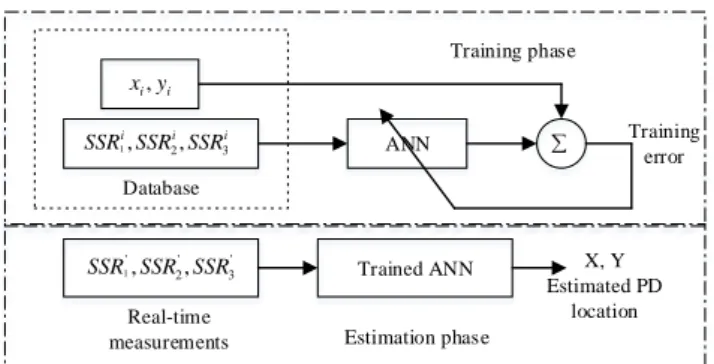
The MLP network consists of an input layer, hidden layer(s) and an output layer. An MLP with a single hidden layer can be represented graphically as shown in Fig. 1. A sigmoidal activation function is used in the hidden layer to provide robustness against outliers and a linear activation function in the input and output layers. The MLP-type ANN is based on the back propagation [24] training of error estimate. It is generally an iterative non-linear optimisation technique. In this study, the MLP approach has been processed in two phases: a training phase and location estimation phase. During the training phase, the MLP network is trained to form a set of fingerprints as a function of PD location.
Input layer Output layer Hidden layer . . . . . . O u tp u t Input vector Fig. 1. MLP Architecture
3 i i i SSR SSR SSR1, 2, 3 ' 3 ' 2 ' , , 1 SSR SSR SSR i i y x, Trained ANN ANN Training error Database Real-time measurements X, Y Estimated PD location Training phase Estimation phase
Fig. 2. MLP model for PD localisation
A set of training examples (fingerprint (RSS) and their corresponding locations) is applied to the network to learn the relation between fingerprints and their locations. This involves tuning the values of the weights and biases of the network to optimise network performance. The batch mode training is implemented in this work. All the inputs in the training set are applied to the network before weights are adjusted to minimise the error between the network output and the desired output. The MLP model developed for PD localisation is as shown in Fig. 2.
During the estimation phase, the PD signal strength values from unknown locations are applied to the input of the trained network to give output corresponding to the PD location. To develop an appropriate MLP model for PD localisation, cross validation is used to determine a suitable network structure in terms of number of hidden neurons. The available training data is randomly partitioned into k disjointed sets. The network is trained for each set of parameters, on all the subsets except for one and the validation error is measured on the subset left out. The procedure is repeated for a total of k trials, each time using a different subset for validation. The average of MSE under validation represent the performance of the network. This process is repeated for different network architecture in terms of number of hidden neurons. The 3-4-2 network model with 3 inputs nodes, 4 hidden neurons and 2 outputs nodes has the best performance and is adopted in this work. In order to improve the generalisation of the model (that is model’s ability to do well on unseen data rather than just training set) and avoid overfitting, Bayesian regularisation [23] is used to train the network.
3.1.2 Radial Basis Function Network Method
Radial Basis Function (RBF) networks are ANNs that have single hidden layer with nonlinear radial basis function. The general structure of an RBF network is shown in Fig. 3 In this work, the RBF network architecture used for PD localisation consist of three inputs, corresponding to the RSS measurement data from the three sensors, a hidden layer and an output layer with two neurons, representing PD location coordinates
(
x
,
y
)
. The structure of a fully connected PD localisation RBF network is as shown in Fig. 4. A radial basis type activation function (Gaussian function) is used for neurons in the hidden layer and a linear activation function for the output layer. The fully connected RBF network is used to approximatef
R
MQ
L
, amapping of PD RSS fingerprints onto PD locations in the physical space.
Fig. 3. General RBFN Architecture
The RBF network consist of two phases: a learning phase and an estimation phase. In the learning phase, the RBF network is trained to form a set of RSS fingerprints as a function of PD location. Each fingerprint is applied to the input of the network and corresponds to the measured RSS-location data. The weights between the hidden layer and the output layer are iteratively adjusted to minimise location error. In the real-time estimation phase, measured PD RSS is applied to the input of the RBF network (acting as a pattern matching algorithm). The output of the RBF network which is the weighted sum of the radial basis function is the PD location estimate.
Given a PD fingerprint r(RSS), the estimated location
l
ˆ
given by the weighted sum of Gaussian basis function [25] is
H k k ku
r
h
w
r
f
r
l
1)
(
)
(
)
(
ˆ
(2)Where
(
r
h
k)
exp(
r
h
k 2)
is the Gaussianradial basis function.H is the number of neurons (basis functions) in the hidden layer which corresponds to the number of training samples,
h
kis the 3-dimensional center for hidden layer neuronk
, andw
kare the 2-dimensional weights for the linear output layer.
is the spread or width of the Gaussian function. For improved performance, the normalized basis function can be used in the model. The weights can be determined in order to optimize the model.
4 Each fingerprint defines the center of a neuron and the width
is obtained via cross validation. Thus, forming the following set of equations;
H k k i k iw
u
r
l
m
h
i
L
m
M
l
1...
,
1
,
,
...
,
1
),
)
,
(
(
(3) This system of linear equations can be written in matrix form asUw
d
and the weights are easily obtained by.
1d
U
w
U
{
u
(
r
j
h
i)
(
j
,
i
)
1
,
...,
R
}
and)
(
u
is the normalised Gaussian basis function. The computed weights are then used during the estimation phase to locate PD. RBF networks suffer from high memory requirements since all reference fingerprints are used as centers for the basis functions and required for localisation.3.2 Support Vector Machine
Support Vector Machines (SVM) [3] [27] [28] are kernel-based learning techniques applicable to both classification and regression problems. SVMs are based on the idea of mapping the original input data point to a high dimensional feature space where a separating hyper-plane can be easily identified. SVMs have shown tremendous success in applications such as data classification, time series prediction, identification systems and data clustering [28] [29] [30] [31] [32]. In the context of PD localisation, SVM is formulated as a regression task, which consist of training a model that defines the non-linear mapping function between the PD RSS and its geo-spatial location in high dimensional feature space, leading to Support Vector Regression (SVR) [33] [34] [35].
3.2.1 Support Vector Regression:
3.2.1.1 Theory of SVR
The support vector regression technique is a learning procedure based on statistical learning theory which employs structural risk minimisation principles [33]. SVR uses training data to build its prediction model. This method can solve both linear and nonlinear regression problems. If the training samples are nonlinear, SVR maps the samples into a high-dimensional feature space by a nonlinear mapping function, where samples become linearly separable and the optimal regression surface is constructed [36]. Given our training dataset of RSS values and locations
)}
,
{(
r
il
iD
withr
i
R
andl
i
L
, the goal of SVR is to find the mappingf
R
L
and makef
(
r
i)
~
l
i, wherer
is input feature vector. For nonlinear problem, the training patterns are pre-processed by a map into some feature space before SVR is applied. SVR finds the best or optimal regression surfacef
(
r
)
within a deviation
as the prediction model, leading to epsilon-SVR [37]. The model can be expressed asb
r
w
r
f
(
)
,
,w
n,
b
(4)Where
.,
.
denotes the dot-product and w and b are the support vector weight and bias respectively. A small w is desired to get an optimal regression surface. This can be achieved by solving the following optimisation problem with the training dataD
[
R
,
L
]
:
i i i il
b
r
w
b
r
w
l
to
subject
w
,
,
min
12 2 (5)Where
w
2
w
,
w
.
The problem in (5) might be restrictive by bounding the range of errors of the training data within
. Thus, to deal with otherwise infeasible constraints, introduce slack variables
i,
i* for each point. The slack variables allow errors to exist up to the value ofi
and
i* without degrading performance. With slack variables the problem becomes [38]:
0
,
,
,
)
(
min
* * 1 * 2 2 1 i i i i i i i i N i i il
b
r
w
b
r
w
l
to
subject
C
w
(6)Where C is the box constraint, a positive numeric value that controls the penalty imposed on data points that lie outside the
margin and helps to prevent overfitting (regularisation). To solve the problem in (6), a standard dualisation method with Lagrange multipliers
i,
i* can be used [36]. By solving the dual problem,w
can be expanded as
N i i i ir
w
1 *)
(
(7)Where
i
0
and
i*
0
. Substituting (7) in (4), andreplacing the dot-product
.
,
.
with a kernel function)
,
(
r
r
k
i [38] to simplify the nonlinear mapping from the input space to the feature space in SVR, the model can be expressed as
N i i i ik
r
r
b
r
f
1 *)
,
(
)
(
)
(
(8) i
are the Lagrange multipliers which satisfyC
i
*0
,r
i are the support vectors whose
i is not zero, andN
is the number of support vectors. Equation (8) shows that the decision function depends on support vectors. This means optimal regression surface is constructed by these support vectors. The idea of support vectors form a sparse subset of the training data that can be used and is5 particularly useful for resource constraint applications such
as the one under investigation.
3.2.1.2 PD Localisation based on SVR
In PD localisation problem, sensors are deployed at arbitrary but known locations in a two-dimensional substation compound; these sensors record radio emission from PD sources in real-time and estimate the location of the PD. The compound is divided into a
1
1
squared grid. Each grid point represented by x-y coordinate is considered a PD location (source). Therefore, to compute PD location, two SVR models are required; one for each x-y coordinates The PD features/patterns used to develop the SVR models is the received signal strength. Firstly, RSS from known locations are gathered by the three sensors deployed in the substation compound. These RSS and their locations form a database for the compound. Suppose the true coordinates of PD locationl
i are(
x
i,
y
i)
and the corresponding values of RSS for the PD from this location are(
r
i1,
r
i2,
r
i3)
.The vector
[
1,
2,
3]
i i i i
r
r
r
R
is taken as the SVR input feature vector and used to infer the locationl
i(
x
i,
y
i)
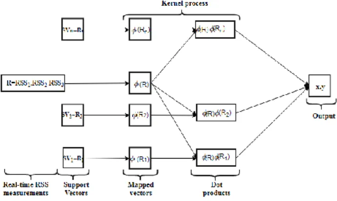
. All the feature vectors from known locations and their corresponding location coordinates constitute the SVR training sample set. Using this training set, the SVR is trained to build a PD localisation models that would subsequently be used to predict or estimate PD location given RSS vector. During training, the input features (RSS) from each known location are transformed to a new feature space with N features, one for each support vector. That is to say that, they are represented only in terms of their dot products with support vectors (special data points chosen by the SVR optimisation algorithm). Gaussian kernel function is employed in the transformation to provide a nonlinear mapping from the input space to the new feature space. In the location estimation phase, for a given RSS vector the kernel finds the similarity or a distance measure between the vector and the support vectors stored after training. The corresponding coordinates of the support vectors closest to the RSS vector are used to compute the PD location for the given RSS vector. The SVR PD location model is as shown in Fig. 5.Fig. 5. SVR PD Localisation model
However, when the electromagnetic environment changes due to external influences, for example change in the location of an electrical equipment, the localisation model would be retrained by the latest collected data. The retraining process can be done automatically, triggered by the location error analysis. If the location error exceeds a predefined threshold, the retraining begins.
The optimal combination of the RBF kernel based SVR hyper-parameters (kernel parameter, insensitive loss function and regularisation parameter) is obtained via cross validation/grid search method.
3.2.2 Least Squares Support Vector Regression:
Least squares support vector regression (LSSVR) algorithm [32] [39] is a reformulation of the standard SVR algorithm described in section 3.2.1.1, which leads to solving a system of linear equations. The idea of linear equations makes LSSVR more appealing and computationally more economical compare to solving the convex quadratic programming (QP) for standard SVR. LSSVR algorithm for PD localisation consist of two phases: Training and Localisation. During the training phase, the parameters of LSSVR algorithm are estimated using PD measurements at known locations (training points). In the localisation phase, PD measurements taken at unknown locations are analysed, and their locations obtained using the parameters estimated in the training phase. Given a training data set
n n nl
r
l
r
l
r
,
),
(
,
),
.
.
.,
(
,
)}
{(
1 1 2 2 of n points, withPD input (RSS) data
r
i
n, and output (PD location coordinate) datal
i(
x
i,
y
i)
2 in 2-dimension, the LSSVR based PD location optimisation problem in the primal weight space is formulated as:
n i i e b wJ
w
e
w
e
1 2 2 1 2 2 1 , ,(
,
)
min
(9) s.tn
i
e
b
r
w
l
i
,
(
i)
i,
1
,...,
with
(
)
:
n
nha function which non-linearly map the input space into the so-called higher dimensional feature space, weight vector
w
nh in primal weight space, bias term b and error variablee
k
. The error term here represents the true deviation between actual PD location and estimated location, rather than a slack variable which is needed to ensure feasibility (as in SVR case).
0
is a regularisation constant.To solve the optimisation problem in the dual space, one defines the Lagrangian
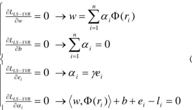
n i i i i T i w r b e l e w J e b w L 1 } ) ( { ) , ( ) ; , , ( (10)with Lagrange multipliers
i
. The conditions for optimality are given by6
0
)
(
,
0
0
0
0
)
(
0
1 1 i i i L i i e L n i i b L n i i i w Ll
e
b
r
w
e
r
w
i S VR LS i S VR LS S VR LS S VR LS
(11)After eliminating w and e, the solution yields the following linear equations:
l
b
v T v0
1
1
0
1
(12) wherel
(
l
1,...,
l
n)
T,
1
v
(
1
,...,
1
)
T and T n)
,...,
(
1
the Lagrange multipliers. Appling Mercer’s condition [32] , the ik-th element of is given by
ik
(
r
i)
T
(
r
k)
K
(
r
i,
r
k)
i
,
k
1
,...,
n
, where is a positive definite matrix and ik-th element of the matrix
ik
K
(
r
i,
r
k)
is a symmetric, continuous function. The resulting LSSVR model for PD location estimation becomes:
n i i i iK
r
r
b
r
f
1)
,
(
)
(
(13)where
,
b
are obtained during the training phase by solving (10). In LSSVR, there are only two parameters to be tuned: the kernel setting and the regularisation constant. Cross-validation/grid search is used to determine the optimal combination of the parameters.4. Experimental Procedure
4.1 Experimental Set Up
In order to verify the effectiveness of the PD localisation system that is based on the deployment of a network of sensor nodes, a systematic test experiment was conducted in a 19.20m x 8.40m laboratory at the University of Strathclyde.
Fig. 6. Measurement grid for measurement campaign
The laboratory contained a great deal of clutter including metallic objects which gives rise to a multipath rich radio environment. Within the accessible area of the laboratory, 144 distinct training locations and 32 testing locations were uniformly selected to form a grid such that the spacing between adjacent training locations is 1 m and the spacing between a training location and its nearest testing location is 0.7 m which represent an array of sensor nodes. Pulse emulated PD sources were set up and 20 RF PD measurements collected at each training and testing location, resulting in 2880 training and 640 testing cases. In real life however, the electrical equipment in which PDs are most likely to appear are not evenly arranged in substations. Given that machine learning algorithms should be trained with representative data, this implies more training samples should be taken where PD is most likely to occur. In practice this would be achieved by positioning a greater concertation of sensor nodes in these areas. An interpolation algorithm can be explore to automatically estimate PD signal strength at unobserved locations based on the representative data. The training process would be repeated at regular intervals such that any changes in the radio environment (due to changes in substation topography) can be incorporated into the model.
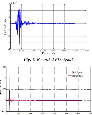
The duration and the repetition frequency of the discharge pulses were 10ps and 100 kHz respectively. Three omnidirectional antennas used for capturing the RF signals were deployed at predefined locations. The arrangement of this procedure is shown in Fig. 6. A high-speed multichannel oscilloscope with memory function was used as a signal-acquisition system to capture and store the PD traces. The oscilloscope has a bandwidth of 9GHz. The PD data acquired from measurement were sampled at 2GS/s. A sample waveform of the received PD signals is shown in Fig. 7. The injected PD pulse waveform and the sensor response are shown in Fig. 8.
4.2Data Preparation
RF signals collected during the measurement campaign are corrupted by noise/interference and this needs to be removed before the PD signals are analysed. In this work, the process of noise removal is accomplished using a wavelet multivariate noising technique [6]. This de-noising scheme combines the decomposition of information given by wavelet transform and the ability of decorrelation among variables given by the Principal Component Analysis (PCA) [40]. The objective is to obtain better de-noised data so as to extract meaningful information from the raw data for PD location. The energy (defined here as the signal strength) contained in each PD trace is then calculated. The average of the 20 individual measurements taken at each training and test locations is computed. Fig. 9 shows PD signal strength variation with respect to location for each of the antennas. The unique signatures created by PD signal strength at different locations facilitate the application of machine learning algorithms for PD localisation. In order to provide more robustness to our system, the ratio of the averaged signal strength components between pairs of receiving antennas is computed and used as fingerprint input vectors to the developed models.
7 Fig. 7. Recorded PD signal
Fig. 8. Response of the receiver sensor for the injected PD
pulse
Fig. 9. Spatial variation of RSS for each antenna
5. Results and Discussions
The performance of SVM-based models (SVR and LSSVR) on the PD data collected is presented and compared with the ANN method. The empirical evaluation of the models is based on statistical operators of location error as well as their cumulative distribution functions (CDFs).
Fig. 10. Model localisation error in x-coordinate The localisation error is computed as the Euclidean distance between the true location and the estimated location of the PD source. CDF describes the probability of locating PD within a specify range of localisation error. This shows how consistent the models perform and capture both the accuracy and precision of the models.
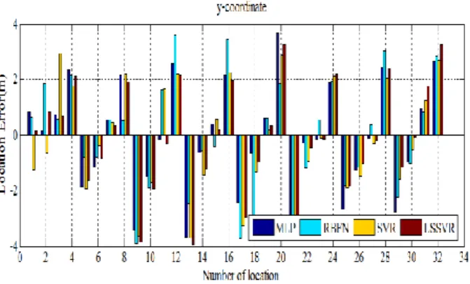
Fig. 10 and Fig. 11 show the errors in each coordinate (x and y) of the test locations for the three models. This result shows that the location errors in x and y vary from -3.5 m to 1.9 m and -3.7 m to 3.7 m respectively for the MLP model and from -5.2 m to 2.3 m in x and -3.9 m to 3.6 m in y for RBFN. For SVR model, the errors in x and y vary from -3.4 m to 1.5 m and -3.7 m to 2.9 m respectively. The result for LSSVR model is similar to that for the other models with errors in x and y varying from -3.3 m to 1.5m and -3.9 m to 3.3 m respectively. It is observed that the overall accuracy of each of the models will be affected mostly by the y-coordinate predictions.
Fig. 12 shows the localisation error in Euclidean distance for each test location. The maximum localisation error for MLP, RBFN, SVR and LSSVR models is found to be 3.90 m, 6.20 m, 4.5 m and 3.99 m respectively with LSSVR model producing location estimate with the lowest error of 0.2 m. Fig. 13 shows CDFs of localisation error for the models. The LSSVR model has a precision of 72 % within 2.5 m compare to SVR, RBFN and MLP models with precision of 69 %, 54% and 60 % within 2.5 m respectively. In other words, the localisation error is less than 2.5 m with probability of 72 %, 69 %, 54% and 60 % for LSSVR, SVR, RBFN and MLP respectively. 0 500 1000 1500 2000 2500 3000 3500 -4 -3 -2 -1 0 1 2 3x 10 -3 Time (ns) A mp lit ud e (mV )
8 Fig. 11. Model localisation error in y-coordinate
Fig. 12. Model localisation errors
Fig. 13. CDF of model localization errors
Fig. 14. Model location accuracy
Table. 1. Cumulative error probability of model location
error
MLP RBFN SVR LSSVR CEP=0.25 1.09 1.40 1.43 1.46 CEP=0.50 2.14 2.43 2.03 1.97 CEP=0.75 2.83 3.39 2.76 2.94
Comparison of the performance of the models based on localisation error corresponding to 0.25, 0.50, and 0.75 overall cumulative error probabilities (CEP) is presented in Table. 1. This clearly shows that half of the time PD sources were located with error less than 2 m when LSSVR algorithm is used for localisation.
The results of localisation accuracy for the models are shown in Fig. 14. It is clear that there is a steady improvement in location accuracy in terms of median error when the SVM-based models are used compared to ANN models. LSSVR model particularly shows an 8.32 % and 22.8 % reduction in median location error when compared with MLP and RBFN models respectively.
6. Conclusion
Machine learning technique for locating PD sources
based on RSS measurement have been considered. The principle and computational realisation of the methods based on support vector machine have been described. Support vector regression (SVR) as well as least squares support vector regression (LSSVR) approach uses the spatial pattern of received signal strength to construct a regression surface in a high dimensional feature space where PD location is determined. This approach models PD location as a linear combination of RSS measurement. In this study, signal strength ratio is used as location fingerprints rather than absolute RSS. The performance of the proposed methods have been evaluated and compared with ANN in terms of statistical operators of localisation error. The results indicate that SVM-based approaches are superior to ANN in accuracy showing a reduction in median location error and represent practical alternatives for PD source localisation. It is believed that the superior performance of SVM-based approaches is due to their ability to converge to a global minimum whereas neural networks are susceptible to converging to local minima. Given the rich complexity of the underlying radio environment convergence to a local minima is highly likely; therefore, SVM-based approaches are more appropriate in this environment. This PD localisation system can monitor and locate discharges from several items of plant concurrently making it suitable for substation-wide PD localisation.7. Acknowledgments
The authors acknowledge the Engineering and Physical Sciences Research Council for their support of this work under grant EP/J015873/1 and Tertiary Education Trust Fund (TETFund) Nigeria.
8. References
[1] Hou, H., Sheng, G., Jiang, X.: “Localization algorithm for the PD source in substation based on L-shaped antenna array signal processing,” IEEE Trans. on Power Del., vol. 30, no. 1, pp. 472--479,
9
2015.
[2] Illias, H. A., Tunio, M. A., Bakar, A. H. A., et al.: “Partial discharge phenomena within an artificial void in cable insulation geometry: experimental validation and simulation,” IEEE Trans. on Dielectr. and Electr. Insul., vol. 23, no. 1, pp. 451--459, 2016.
[3] Rostaminia, R., Saniei, M., Vakilian, M., et al.: “Accurate power transformer PD pattern recognition via its model,” IET Science, Meas. & Tech., vol. 10, no. 7, pp. 745-753, 2016.
[4] Moore, P. J., Portugues, I. E., Glover, I. A.: “Partial discharge investigation of a power transformer using wireless wideband radio-frequency measurements,” IEEE Trans. on Power Del., vol. 21, no. 1, pp. 528--530, 2006.
[5] Mohamed, F. P., Siew, W.H., Soraghan, J.J.: “Online partial discharge detection in medium voltage cables using protection and instrument current transformers,” 2nd UHVNet Colloquium on high voltage
measurement and insulation research, Glasgow, 2009.
[6] Evagorou, D., Kyprianou, A., Lewin, P.L. et al.: “Feature extraction of partial discharge signals using the wavelet packet transform and classification with a probabilistic neural network,” IET Science, Meas.& Tech., vol. 4, no. 3, pp. 177-192, 2010.
[7] Lu, Y., Tan, X., Hu, X.: “PD detection and localisation by acoustic measurements in an oil-filled transformer,” IEE Proceedings - Science, Meas. & Tech., vol. 147, no. 2, pp. 81-85, 2000.
[8] Li, P., Zhou, W., Yang, S., et al.:, “Method for partial discharge localisation in air-insulated substations,” IET Science, Meas. & Tech.,
2017.
[9] Mohamed, F. P., Siew, W. H., Soraghan, J. J., et al.: “Remote monitoring of partial discharge data from insulated power cables,”
IET Science, Meas. & Tech., vol. 8, no. 5, pp. 319-326, 2014.
[10] Portugues, I. E., Moore, P. J., Glover, I. A., et al.: “RF-based partial discharge early warning system for air-insulated substations,” IEEE Trans. on Power Del., vol. 24, no. 1, pp. 20--29, 2009.
[11] Hou, H., Sheng, G., Miao, P., et al.:“Partial discharge location based on radio frequency antenna array in substation,” High Voltage Eng.,
vol. 38, no. 6, pp. 1334-1340, 2012.
[12] Tang, J., Xie, Y.: “Partial discharge location based on time difference of energy accumulation curve of multiple signals,” IET Electric Power App., vol. 5, no. 1, pp. 175-180, 2011.
[13] Hou, H., Sheng, G., Jiang, X.: “Robust Time Delay Estimation Method for Locating UHF Signals of Partial Discharge in Substation,”
IEEE Trans. on Power Del., vol. 28, no. 3, pp. 1960-1968, 2013.
[14] Judd, M. D.:, “Radiometric partial discharge detection,” Int. Conf. on Condition Monitoring and Diagnosis, Beijing, 2008.
[15] Portugues, I. E., Moore , P. J., Carder, P.: “The use of radiometric partial discharge location equipment in distribution substations,” 18th Int. Conf. and Exhibition on Electricity Distribution, Turin, 2005.
[16] Zhu, M. X., Wang, Y. B., Liu, Q., et al.: “Localization of multiple partial discharge sources in air-insulated substation using probability-based algorithm,” IEEE Trans. on Dielectr. and Electr. Insul., vol. 24, no. 1, pp. 157-166, 2017.
[17] Hooshmand, R. A., Parastegari M., Yazdanpanah, M.: “Simultaneous location of two partial discharge sources in power transformers based on acoustic emission using the modified binary partial swarm optimisation algorithm,” IET Science, Meas. & Tech., vol. 7, no. 2, pp. 112-118, 2013.
[18] Boya, C., Rojas-Moreno, M. V., Ruiz-Llata, M., et al.: “Location of partial discharges sources by means of blind source separation of UHF signals,” IEEE Trans. on Dielectr. and Electr. Insul., vol. 22, no. 4, pp. 2302--2310, 2015.
[19] Sinaga, H. H., Phung, B. T. Blackburn, T. R.: “Partial discharge localization in transformers using UHF detection method,” IEEE Trans. on Dielectr. and Electr. Insul., vol. 19, no. 6, pp. 1891--1900, 2012.
[20] Iorkyase, E. T., Tachtatzis, C., Atkinson, R. C., et al.: “Localisation of partial discharge sources using radio fingerprinting technique,”
Loughborough Antennas Propag. Conf. (LAPC), Loughborough, 2015.
[21] Genming, D., Zhang, J., Zhang, L., et al.: “Overview of received signal strength based fingerprinting localization in indoor wireless LAN environments,” IEEE 5th International Symposium on Microwave, Antenna, Propagation and EMC Technologies for
Wireless Communications (MAPE), 2013.
[22] Chuang, P. J., Jiang, Y. J.: “Effective neural network-based node localisation scheme for wireless sensor networks,” IET Wireless Sensor Systems, vol. 4, no. 2, pp. 97-103, 2014.
[23] Roj, J.: “Estimation of the artificial neural network uncertainty used for measurand reconstruction in a sampling transducer,” IET Science, Meas. & Tech., vol. 8, no. 1, pp. 23-29, 2014.
[24] Mohanty, S., Ghosh, S.: “Artificial neural networks modelling of breakdown voltage of solid insulating materials in the presence of void,” IET Science, Meas. & Tech., vol. 4, no. 5, pp. 278-288, 2010.
[25] Laoudias, C., Kemppi, P., Panayiotou, C. G.: “Localization using radial basis function networks and signal strength fingerprints in WLAN,” IEEE Global telecomm. conf., Honolulu, 2009.
[26] Nerguizian, C. , Despins, C., Affes, S.: “Indoor geolocation with received signal strength fingerprinting technique and neural networks,” Int. Conf. on Telecomm., Berlin, 2004.
[27] Jiang, E., Zan, P., Zhu, X., et al.: “Rectal sensation function rebuilding based on optimal wavelet packet and support vector machine,” IET Science, Meas. & Tech., vol. 7, no. 3, pp. 139-144, 2013.
[28] Hao, L., Lewin, P. L.: “Partial discharge source discrimination using a support vector machine,” IEEE Trans. on Dielectr. and Electr. Insul.,
vol. 17, no. 1, pp. 189--197, 2010.
[29] Ravikumar, B., Thukaram, D., Khincha, H. P.: “Application of support vector machines for fault diagnosis in power transmission system,” IET Gen., Transm. & Distr., vol. 2, no. 1, pp. 119-130, 2008.
[30] Khan, Y., Khan, A. A., Budiman, F. N., et al.: “Partial discharge pattern analysis using support vector machine to estimate size and position of metallic particle adhering to spacer in GIS,” Electric Power Systems Research, vol. 116, pp. 391--398, 2014.
[31] Ben-Hur, A., Horn, D., Siegelmann, H. T., et al.: “Support vector clustering,” The Journal of Machine Learning Research, vol. 2, pp. 125--137, 2002.
[32] Bessedik, S. A., Hadi, H.: “Prediction of flashover voltage of insulators using least squares support vector machine with particle swarm optimisation,” Electric Power Systems Research, vol. 104, pp. 87-92, 2013.
[33] Basak, D., Pal, S., Patranabis, D. C.: “Support vector regression,”
Neural Infor. Processing-Letters and Reviews, vol. 11, no. 10, pp. 203--224, 2007.
[34] Zhang, H. R., Wang, X. D., Zhang, C. J., et al.: “Robust identification of non-linear dynamic systems using support vector machine,” IEE Proceedings - Science, Meas. & Tech., vol. 153, no. 3, pp. 125-129, 2006.
[35] Clarke, S. M., Griebsch, J. H., Simpson, T. W.: “Analysis of support vector regression for approximation of complex engineering analyses,” Journal of Mechanical Design, vol. 127, no. 6, pp. 1077--1087, 2005.
[36] Shi, K., Ma, Z., Zhang, R., et al.: “Support Vector Regression Based Indoor Location in IEEE 802.11 Environments,” Mobile Infor. Systems, vol. 2015, p. 14, 2015.
[37] Bennett, K. P., Campbell, C.: “Support vector machines: hype or hallelujah?,” ACM SIGKDD Explorations Newsletter, vol. 2, no. 1, pp. 1-13, 2000.
[38] Junshui, M., James, T., Simon, P.: “Accurate On-line Support Vector Regression,” Neural Comput., vol. 15, no. 11, pp. 2683--2703, 2003.
[39] Wu, Z., Li, C., Yang, Z., et al.: “Research on tourists' positioning technology based on LSSVR,” IEEE Advanced Infor. Tech., Electronic and Automation Control Conf., Chongqing, 2015.
[40] Mohanty, S., Gupta, K. K., Raju, K. S.: “Adaptive fault identification of bearing using empirical mode decomposition-principal component analysis-based average kurtosis technique,” IET Science, Meas. & Tech., vol. 11, no. 1, pp. 30-40, 2017.