Improving Deep Representation Learning with Complex and Multimodal Data.

(1)

Improving Deep Representation Learning

with Complex and Multimodal Data

by Kihyuk Sohn

A dissertation submitted in partial fulfillment of the requirements for the degree of

Doctor of Philosophy (Electrical Engineering:Systems)

in the University of Michigan 2015

Doctoral Committee:

Assistant Professor Honglak Lee, Chair Professor Alfred O. Hero III

Professor Benjamin Kuipers

(2)

(3)

(4)

ACKNOWLEDGEMENTS

First of all, I would like to express my sincere gratitude to my advisor, Professor Honglak Lee, for his guidance, encouragement and continuous support throughout my graduate studies. Luckily for me, I was admitted as his first Ph.D. student when he started his career as an assistant professor at the University of Michigan, and had more than enough opportunities to discuss, execute, and publish our work over the years. All my achievements have benefited from his knowledge, insight and inspiration. I would like to extend my appreciation to other members of my dissertation committee, Professor Alfred O. Hero III, Professor Benjamin Kuipers, and Professor Clayton D. Scott for their motivating suggestions and valuable comments. My thanks also extend to many other faculty members and staffs in the Department of Electrical Engineering and Computer Science for their teaching, advice and kindness.

My sincere appreciation is extended to Professor Erik G. Learned-Miller of the Uni-versity of Massachusetts Amherst for his invaluable advice and support, which played a crucial role in motivating the second part of the Ph.D. thesis. Many thanks to my colleagues, Scott Reed, Yuting Zhang, Wenling Shang, Ruben Villegas, Junhyuk Oh, Xinchen Yan, Ye Liu, Guanyu Zhou, Chansoo Lee (from UM machine learning group), and Andrew Kae (from UMass), for their valuable discussions and warm friendship. To my friends that I have met in Ann Arbor, thanks for the memories and great times we shared over the years. Specifically, I would like to thank Sungjoon Park, Donghwan Kim, Dae Yon Jung, Kyunghoon Lee and the members of “Invaders”, Jongjin Park, Taehyung Kim, Yelin Kim, who shared my 7 years of journey at Michigan from

(5)

begin-ning to end. I am also thankful to Gyouho Kim, Suyoung Bang, and the members of our football club “A.K. United” for our team workouts and other moments we shared. I am truly indebted to the members of Korean Presbyterian Church of Ann Arbor, including Pastor Jae Joong Hwang, executive board members, Hyungmin Baek, Hanna Song, Myungjoon Choi, and the “For God” worship team and the “Hesed” choir team, who helped enriching my life in God.

I would like to express my deepest gratitude to my family for their countless love and support. My parents have always been a source of comfort and hope in difficult times. I also thank my sister, brother-in-law, and my lovely nephew, Onew Yang, for being there. Your presence has been great pleasure and encouragement.

Lastly, I gratefully acknowledge the financial support from the National Science Foundation (contract No. 1247414), Office of Naval Research (contract No. N00014-13-1-0762) and Samsung Digital Media and Communication Lab, and the donation of GPUs from NVIDIA.

(6)

LIST OF FIGURES

Figure

2.1 Pipeline for constructing features in object recognition. . . 12 2.2 Illustration of CRBM.NV andNH refer to the size of visible and hidden

layer, and ws to the size of convolution filter. The convolutional filter for the l-th channel (of size ws ×ws) corresponding to k-th hidden group is denoted as Wk,l. . . 15

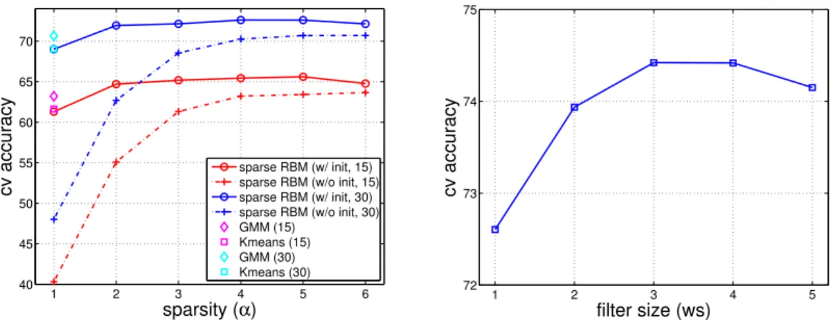
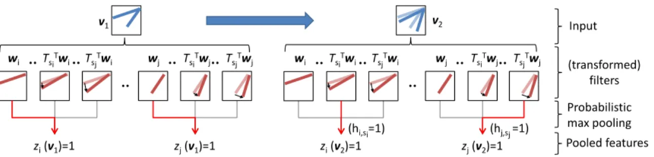
2.3 (Left) Average cross-validation accuracy on Caltech 101 dataset with 1024 bases using K-means, GMM, and sparse RBM with different spar-sity values. The “sparse RBM (w/ init)” denotes the sparse RBM ini-tialized from GMM as described in Section 2.4; the “sparse RBM (w/o init)” denotes the sparse RBM initialized randomly (baseline). Blue and cyan represent settings with 30 training images per class. Red and magenta represent settings with 15 training images per class. (Right) Average cross-validation accuracy on the Caltech 101 dataset with 1024 bases and different convolution filter sizes (ws). . . 27 3.1 Feature encoding of TI-RBM. Shaded pattern inside thev2 reflects the

v1, while the shaded patterns in transformed filters show the

corre-sponding original filters wi or wj. The filters selected via probabilistic

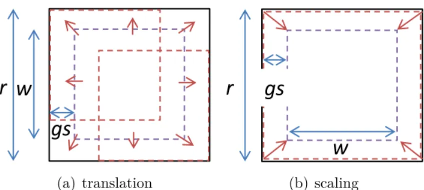
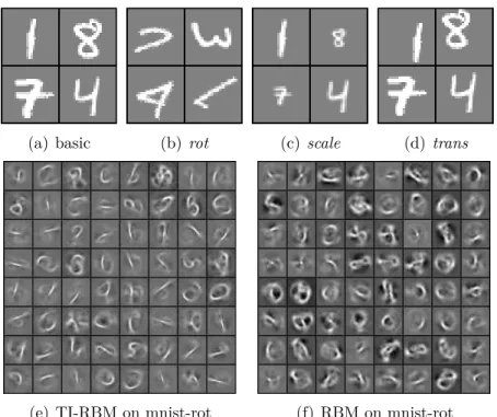
max pooling across the set of transformations are depicted in red arrows (e.g., in the rightmost example, the hidden unit hj,sj corresponding to the transformation Tsj and the filter wj contributes to activate zj(v2).) 32 3.2 Translation and scale transformations on images. . . 36 3.3 (top) Samples from the handwritten digit datasets with (a) no

trans-formations, (b) rotation, (c) scaling, and (d) translation. (bottom) Learned filters from mnist-rot dataset with (e) the sparse TI-RBM and (f) the sparse RBM, respectively. . . 38 3.4 Visualization of filters trained with RBM and TI-RBMs on natural

images. We trained 24 filters and used nine translations with a step size of 1 pixel, five rotations with a step size ofπ/8 radian, and two-level scale transformations with a step size (gs) of 2 pixels, respectively. . . . 39

(11)

4.1 Graphical model representation of the (a) PGBM and (b) supervised PGBM with two groups of hidden units. The Bernoulli switch unit zi

specifies which of the two components models the visible unit vi. In

other words, when zi = 1, vi is generated from the hidden units in the

first group (shown in red); whenzi = 2,vi is generated from the hidden

units in the second group (shown in green). . . 49 4.2 Visualization of (a, b) filters corresponding to two components learned

from the PGBM, (c) activation of switch units, and (d) corresponding original images on bg-image dataset. Specifically, (a) represents the

group of hidden units that activates for the foreground digits (task-relevant), and (b) represents the group of hidden units that activates for the background images (task-irrelevant). See text for details. . . . 54 4.3 Architecture of the two-layer CPGDN model. We use the CRBM for

the first layer, and the CPGBM with two mixture components for the second layer. We also visualize the filters for each mixture component learned from the “Face” category. In this figure, we use ¯z for binary variable z to denote its complement, i.e., ¯z = 1−z. . . 61 4.4 Visualization of the second layer CPGBM features from “Faces” (a, b)

and “Car side” (c, d) classes. . . 62 4.5 Visualization of the pairs of examples for switch unit activation map and

the corresponding image below overlayed with the predicted (red) and the ground truth bounding boxes (green). The first row of examples are generated using the CPGDN trained only on either “Face” (left four examples) or “Car” (right four examples) classes. The second and third rows of examples are generated using the CPGDN trained on all categories of images from Caltech 101 dataset. . . 63 5.1 The left image shows a “funneled” or aligned LFW image. The center

image shows the superpixel version of the image which is used as a basis for the labeling. The right image shows the ground truth labeling. Red represents hair, green represents skin, and the blue represents background. 66 5.2 The GLOC model. The top two layers can be thought of as an RBM

with the (virtual) visible nodes ¯yr and the hidden nodes. To define

the RBM over a fixed-size visible node grid, we use an image-specific “projection matrix” {p(_rsI)} that transfers (top-down and bottom-up)

information between the label layer and the virtual grid of the RBM’s visible layer. See text for details. . . 73 5.3 Generated samples from the RBM (first row) and the closest matching

examples in the training set (second row). The RBM can generate novel, realistic examples by combining hair, beard and mustache shapes along with diverse face shapes. . . 77

(12)

5.4 Sample segmentation results on images from the LFW data set. The images contain extremely challenging scenarios such as multiple distrac-tor faces, occlusions, strong highlights, and pose variation. The left of Figure 5.4(a) shows images in which the GLOC model made relatively large improvements to the baseline. The right of Figure 5.4(a) shows more subtle changes made by our model. The results in Figure 5.4(b) show typical failure cases. The columns correspond to 1) original image which has been aligned to a canonical position using funneling [48], 2) CRF, 3) spatial CRF, 4) GLOC and 5) ground truth labeling. Note that the CRBM model results are not shown here. . . 78 5.5 The filter visualization in each column show that the GLOC model

learns latent structure or visual attribute automatically from the data that can be interpreted as (from left to right) “no hair showing”, “look-ing left”, “look“look-ing right”, “beard/occluded chin”, “big hair”. In each column, we retrieve the images from LFW (except images used in train-ing and validation) with the highest activations for each of 5 hidden units, and provide their segmentation results. Although the retrieved matches are not perfect, they clearly have semantic, high-level content. 82 6.1 An instance of MDRNN with target y given x. Multiple iterations of

bottom-up updates (y → h(3)_{; Equation (6.11) and (6.12)) and}

top-down updates (h(3) _→ _y; Equation (6.13)) are performed. The arrow

indicates encoding direction. . . 94 6.2 Visualization of samples with inferred missing modality. From top to

bottom, we visualize ground truth, left or right halves of digits, gen-erated samples with inferred missing modality using MRBM with ML objective, MinVI objective using CD-PercLoss and MP training methods. 96 6.3 Retrieval results with multimodal queries. The leftmost image-text

pairs are multimodal query samples and those in the right side of the bar are retrieved samples with the highest similarities to the query sample from the database. . . 100 7.1 (a) A graphical model representation of the condVAE describing the

generative (left) and recognition (right) processes, (b) a schematic flowchart of the condVAE during the training, and (c) that of the condVAE with recurrent prediction network. . . 105 7.2 Multi-scale training. . . 109 7.3 Visualization of generated samples with (left) 1 quadrant and (right)

2 quadrants for an input. We show (first) the input and the ground truth output overlaid with gray color, and (second) samples generated by the baseline NNs, and (rest) samples drawn from the condVAEs. . . 111 7.4 Visualization of (first row) input image with omission noise (noise level:

50%, block size: 8), (second row) ground truth segmentation, and (third) prediction by CNN, and (fourth to sixth) the generated samples by condVAE on (left) CUB and (right) LFW database. . . 116

(13)

LIST OF TABLES

Table

2.1 Average test classification accuracy for Caltech 101. . . 24 2.2 Average test classification accuracy for Caltech 256. . . 25 3.1 Test classification error on MNIST transformation datasets. The

best-performing methods for each dataset are shown in bold. . . 37 3.2 Test classification accuracy on CIFAR-10 dataset. 1,600 filters were

used unless otherwise stated. The numbers with † and ‡ are from [21]

and [19], respectively. . . 40 3.3 Test classification accuracy on STL-10. 1,600 filters were used for all

experiments. . . 41 3.4 Phone classification accuracy on the TIMIT core test set using linear

SVMs. . . 42 3.5 Phone classification accuracy on the TIMIT core test set using

RBF-kernel SVMs. . . 43 4.1 Test classification errors of (top) single-layer and (bottom) multi-layer

models on MNIST variation datasets. We used 10,000/2,000/50,000 splits for train, validation and test sets, and report the test classification errors without retraining the model after hyperparameter search over the validation set. For all RBM variants including imRBM, discRBM, and PGBM, we used sparsity regularizer [82]. The best performers among the single-layer models and the deep network models are both in bold. . . 59 4.2 The mean and the standard deviation of the test classification errors of

semi-supervised PGBM, supervised PGBM, RBM, and RBM-FS. We repeated 5 times with randomly sampled 1,000 labeled training exam-ples in addition to the remaining 9,000 unlabeled training examexam-ples. The best model and those within the standard deviation are in bold. . 60 4.3 Test classification accuracy on Caltech 101. . . 62 5.1 Labeling accuracies for each model. We report the mean of

superpixel-wise labeling accuracy and corresponding 95% confidence interval in the second column, and the error reduction over the CRF on test set in the third column. . . 80

(14)

6.1 Test set errors on handwritten digit recognition dataset using MRBMs with different training objectives and learning methods. The joint rep-resentation was fed into linear SVM for classification. . . 96 6.2 Test set mAPs on MIR-Flickr database. We implemented autoencoder

following the description in [99]. Multimodal DBM† _{is supervised}

fine-tuned model. See [122] for details. . . 98 6.3 Validation set mAPs on MIR-Flickr database with different number of

mean-field iterations. . . 99 7.1 The negative CLL on the validation/test sets of MNIST database. We

increase the number of quadrants for an input from 1 to 3, and estimate the CLL using generative sampling by default. The performance gap between the condVAE (IS) and the baseline NN is reported. . . 111 7.2 The negative CLL on CUB database. We used importance sampling to

estimate the CLL of condVAE and hybrid models. . . 112 7.3 Labeling results on CUB database. We report both pixel-wise labeling

accuracy and IoU score of the foreground region. The term “recur.” refers the network with recurrent prediction architecture, which is used as opposed to the “flat”, and “ssc” and “msc” refers single-scale and multi-scale prediction training, respectively. The “NI” refers the noise-injection training. . . 113 7.4 Labeling results and the negative CLL on LFW database. We report

the pixel-wise 4-way (skin, hair, clothes, background) prediction accu-racy. We used recurrent architecture and the models are trained with multi-scale prediction training and noise-injection methods. We used importance sampling to estimate the CLL of condVAE and hybrid models.114 7.5 Interactive segmentation results with input omission noise and weak

supervision on CUB (left) and LFW (right) database. We report the pixel-level accuracy on the first validation set. . . 115

(15)

LIST OF APPENDICES

Appendix

A. Supplementary material of Chapter II . . . 124

B. Supplementary material of Chapter IV . . . 130

C. Supplementary material of Chapter V . . . 134

(16)

ABSTRACT

Improving Deep Representation Learning with Complex and Multimodal Data by

Kihyuk Sohn

Chair: Honglak Lee

Representation learning has emerged as a way to learn meaningful representation from data and made a breakthrough in many applications including visual object recognition, speech recognition, and text understanding. However, learning representation from complex high-dimensional sensory data is challenging since there exist many irrelevant factors of variation (e.g., data transformation, random noise). On the other hand, to build an end-to-end prediction system for structured output variables, one needs to incorporate probabilistic inference to properly model a mapping from single input to possible configurations of output variables. This thesis addresses limitations of current representation learning in two parts.

The first part discusses efficient learning algorithms of invariant representation based on restricted Boltzmann machines (RBMs). Pointing out the difficulty of learning, we develop an efficient initialization method for sparse and convolutional RBMs. On top of that, we develop variants of RBM that learn representations invariant to data transformations such as translation, rotation, or scale variation by pooling the filter responses of input data after a transformation, or to irrelevant patterns such as random or structured noise, by jointly performing feature selection and feature learning. We

(17)

demonstrate improved performance on visual object recognition and weakly supervised foreground object segmentation.

The second part discusses conditional graphical models and learning frameworks for structured output variables using deep generative models as prior. For example, we combine the best properties of the CRF and the RBM to enforce both local and global (e.g., object shape) consistencies for visual object segmentation. Furthermore, we develop a deep conditional generative model of structured output variables, which is an end-to-end system trainable by backpropagation. We demonstrate the importance of global prior and probabilistic inference for visual object segmentation. Second, we develop a novel multimodal learning framework by casting the problem into structured output representation learning problems, where the output is one data modality to be predicted from the other modalities, and vice versa. We explain as to how our method could be more effective than maximum likelihood learning and demonstrate the state-of-the-art performance on visual-text and visual-only recognition tasks.

(18)

CHAPTER I

Introduction

1.1

Motivation

In recent years, representation learning algorithms (e.g., clustering [2, 32, 74, 140], sparse coding [15, 147, 143, 101, 81], restricted Boltzmann machine (RBM) [117], au-toencoders [9, 91, 73, 6], and deep learning [46, 111, 84, 11, 78, 68]) have emerged as a way to learn useful features from unlabeled and labeled data.

Representation learning algorithms can be classified into two categories, supervised and unsupervised learning, depending on the use of supervision during the training. In unsupervised learning, the goal is to learn features that capture underlying struc-tures (e.g., statistical dependencies such as co-occurrence) in data, and feastruc-tures that are learned complement or sometimes outperform manually designed domain-specific features (e.g., SIFT [88], HOG [22] in computer vision, MFCC [23] in speech process-ing). Furthermore, these methods make minimal assumptions about the data, and they have been successfully applied to many tasks in different domains, including vi-sual recognition [68], speech processing [103], and text understanding [34]. However, learning representation from complex unlabeled sensory data is still a very challenging problem due to many reasons; first, raw input data is usually very noisy and highly variable, and does not provide useful information for the target task. Second, there are many factors of variation that are not necessarily relevant to the target tasks, such

(19)

as low-level domain-specific transformation (e.g., pixel-level translation or rotation) or external sources of variation (e.g., lighting condition). To achieve a good recognition performance, it is important to learn robust feature representations that are invariant

to such kinds of irrelevant intrinsic or extrinsic factors of variation. Finally, it is often the case that the unsupervised learning algorithms with high expressive power (e.g., RBM) are difficult to train and thus require much of an expert’s knowledge and efforts to train.

On the other side of the story, the supervised representation learning algorithms have made a significant progress in recent years. Specifically, the convolutional neu-ral network (CNN) has shown impressive performance on large-scale visual recognition tasks [68]. Behind the scenes, there are several ingredients that contributed to make a breakthrough: 1) powerful GPUs that can train very deep (convolutional) neural net-works with a reasonable time cost, 2) huge number of labeled training examples such as the ImageNet database [24], 3) stochastic gradient descent with advanced optimization techniques (e.g., adaptive learning rate schedule algorithms [128, 26], rectified linear units [149, 97], dropout [123]). Although deep neural networks have been so successful for simple recognition tasks, not much has been shown yet for complex structured output prediction problems. Unlike simple recognition problems, the distribution of structured outputs have multiple modes, i.e., there could be several possible outcomes that can be derived from the same input, and deep neural networks, which are extremely powerful function approximators, may not be the optimal for modeling complex outputs. Simi-lar challenge can often be found in multimodal joint representation learning problems, where we have input data from multiple channels during the training. The promise of multimodal representation learning is that the performance improvement is guaranteed over the single data modality counterpart. However, it becomes non-trivial when we have a missing data modality for testing, and it is important to learn a generative model that has an ability to predict or reason about a missing data modality conditioned on

(20)

the observation.

In this thesis, we aim to solve the following research questions to build a robust and intelligent agent that can effectively learn representations from complex and multiple heterogeneous data sources:

1. How to make the learning procedure of the highly expressive representation learn-ing methods a black-box by avoiding extensive hyperparameter search?

2. How to learn representations that are invariant to intrinsic data transformation from complex sensory data?

3. How to learn representations that are robust to irrelevant input patterns or ran-dom noise?

4. How to develop a generic supervised learning algorithm for structured output prediction that incorporates long-range, higher-order interactions among output variables?

5. How to learn a better joint representation of multiple heterogeneous data that can reason about a missing data modality?

6. How to develop an end-to-end system for structured output representation learn-ing and prediction, and multimodal representation learnlearn-ing with deep convolu-tional neural networks?

1.2

Organization of the Thesis

This thesis is organized in 8 chapters including the introduction (Chapter I), and the conclusion and future work (Chapter VIII). The main chapters (II – VII) are divided into 2 parts, 3 chapters each. The first part (Chapter II, III, IV) discusses on efficient learning algorithms of invariant feature representations from complex sensory data. We

(21)

change gears in the second part (Chapter V, VI, VII) towards learning representations of structured output or multimodal data using (a combination of) conditional generative objectives. We briefly state the problem, our approach and contributions for each chapter.

Chapter II. Efficient Learning of Sparse, Distributed, Convolutional Feature Representations for Object Recognition.

Informative feature representations are important for achieving state-of-the-art perfor-mance in machine learning tasks. The RBM has been successfully applied to automati-cally learn useful patterns from large amount of unlabeled data. Although it has a great potential due to its rich expressive power and capability to build a deep network, the difficulty of training RBMs has been a barrier to their wide use. In this chapter, we ad-dress this difficulty by showing the connections between mixture models and RBMs and deriving an efficient training method for RBMs from these connections. Along with this efficient training, we evaluate the importance of convolutional training that can cap-ture a larger spatial context with less redundancy, as compared to non-convolutional training. Overall, our method achieves state-of-the-art performance on visual object recognition benchmarks.

Chapter III. Learning Invariant Representations with Local Transforma-tions.

The difficulty of developing representation learning algorithms that are robust to data transformations (e.g., scale, rotation, or translation) has been a challenge in many applications (e.g., object recognition problems). In this chapter, we address the problem of learning transformation invariant features by introducing the transformation matrices into the energy function of the RBMs. The proposed transformation-invariant RBMs not only learn the diverse patterns by explicitly transforming the weight matrix, but

(22)

they also achieve the invariance of the representation via probabilistic max pooling of hidden units over the set of transformations. We evaluate our algorithm on several benchmark on visual recognition, such as the variations of MNIST, or CIFAR-10 and STL-10, as well as the customized digit datasets with significant transformations, and show competitive classification performance to the state-of-the-art. Besides the image data, we apply our method to phone classification task on the TIMIT database to show the wide applicability of our proposed algorithms to other domains, also achieving state-of-the-art performance.

Chapter IV. Learning and Selecting Features Jointly with Point-wise Gated Boltzmann Machines.

Learning useful high-level features is still challenging when the data contains a sig-nificant amount of irrelevant patterns. In this chapter, we propose a point-wise gated Boltzmann machine, a unified generative model that combines feature learning and

feature selection. Our model performs not only feature selection on learned high-level features (i.e., hidden units), but also dynamic feature selection on raw features (i.e.,

visible units) through a gating mechanism. For each example, the model can adap-tively focus on a variable subset of visible nodes corresponding to the task-relevant patterns, while ignoring visible units corresponding to the task-irrelevant patterns. In experiments, our method achieves improved performance over state-of-the-art in several visual recognition benchmarks.

Chapter V. Augmenting CRFs with Boltzmann Machine Priors for Struc-tured Output Prediction.

CRFs provide powerful tools for building models to label image segments. They are particularly well-suited to model local interactions among adjacent regions (e.g., su-perpixels). However, CRFs are limited in dealing with complex, global (long-range)

(23)

interactions between regions. Complementary to this, RBMs can be used to model global shapes produced by segmentation models. In this chapter, we present a new model that combines these two network types to build a state-of-the-art region labeler. Although the CRF is a good baseline labeler, we show how an RBM can be added to the architecture to provide aglobalshape bias that complements the local modeling

pro-vided by the CRF. We demonstrate the labeling performance for the parts of complex face images from the Labeled Faces in the Wild data set. This hybrid model produces results that are both quantitatively and qualitatively better than the CRF alone. In addition, we demonstrate that the hidden units in the RBM portion of our model can be interpreted as face attributes that have been learned without any attribute-level supervision.

Chapter VI. Improved Multimodal Deep Learning with Variation of Infor-mation.

It is important to capture high-level associations between multiple data modalities with a compact set of latent variables, and deep learning has been successfully applied to this problem of multimodal representation learning. Nonetheless, there still remains an important question how to learn a good association between multiple data modalities, in particular, to reason about the missing data modalities in the testing time. In this chapter, we propose a novel multimodal representation learning objective that explicitly aims this goal. Instead of maximum likelihood learning, we train the networks to minimize thevariation of information, an information theoretic measure that computes

the information distance between data modalities. In experiments, we demonstrate the state-of-the-art visual-textual and visual recognition performance on MIR-Flickr database and PASCAL VOC 2007 database.

(24)

Chapter VII. Learning to Predict Structured Outputs using Stochastic Con-volutional Networks.

To build an end-to-end system for structured output prediction one needs to incorporate probabilistic inference, as it may not be a simple many-to-one function approximation problem (e.g., recognition and classification), but could be a task of mapping input to many possible outputs. In this chapter, we propose a stochastic convolutional neural networks with Gaussian latent variables for structured output prediction and represen-tation learning. In light of recent development in variational inference and learning of directed graphical models [62, 107, 63], we propose a conditional variational auto-encoder (condVAE). We demonstrate the importance of stochastic neurons in modeling the distribution with multiple major modes using the toy example of MNIST database. In addition, we demonstrate the effectiveness of our proposed model on several image segmentation and region labeling database.

1.3

List of Publications

Here, we enumerate the list of publications relevant to each chapter:

[1] Efficient Learning of Sparse, Distributed, Convolutional Feature Representations for Object Recognition. Kihyuk Sohn, Dae Yon Jung, Honglak Lee, and Alfred Hero III. InProceedings of the International Conference on Computer Vision, 2011. (Chapter II)

[2]Learning Invariant Representations with Local Transformations. Ki-hyuk Sohn and Honglak Lee. In Proceedings of the International Conference on Machine Learning, 2012. (Chapter III)

[3]Learning and Selecting Features Jointly with Point-wise Gated Boltz-mann Machines. Kihyuk Sohn, Guanyu Zhou, Chansoo Lee, and Honglak Lee. In Proceedings of the International Conference on Machine Learning, 2013.

(25)

(Chapter IV)

[4]Augmenting CRFs with Boltzmann Machine Shape Priors for Image Labeling. Kihyuk Sohn∗, Andrew Kae∗, Honglak Lee, and Erik Learned-Miller. In Proceedings of the IEEE Conference on Computer Vision and Pattern Recog-nition, 2013 (∗ indicates equal contribution) (Chapter V)

[5]Improved Multimodal Deep Learning with Variation of Information. Kihyuk Sohn, Wenling Shang, and Honglak Lee. In Advances in Neural Infor-mation Processing Systems, 2014 (Chapter VI)

There are few more publications that I have published during my Ph.D. years: [6]Online Incremental Feature Learning with Denoising Autoencoders. Guanyu Zhou, Kihyuk Sohn, and Honglak Lee. In Proceedings of the Interna-tional Conference on Artificial Intelligence and Statistics, 2012.

[7]Learning to Disentangle Factors of Variation with Manifold Interac-tion. Scott Reed,Kihyuk Sohn, Yuting Zhang and Honglak Lee. InProceedings of the International Conference on Machine Learning, 2015.

[8]Improving Object Detection with Deep Convolutional Networks via Bayesian Optimization and Structured Prediction. Yuting Zhang,Kihyuk Sohn, Ruben Villegas, Gang Pan and Honglak Lee. In Proceedings of the IEEE Conference on Computer Vision and Pattern Recognition, 2015

For reproducible research, the code will be made available in my personal website:

(26)

CHAPTER II

Efficient Learning of Sparse, Distributed,

Convolutional Feature Representations

2.1

Introduction

Object recognition poses a significant challenge due to the high pixel-level variability of objects in images. Therefore, having higher-level, informative image features is a nec-essary component for achieving state-of-the-art performance in object classification and detection. In the last decades, many efforts have been made to develop feature repre-sentations that can provide useful low-level information from images [88, 22]. However, these feature representations are often hand-designed and require significant amounts of domain knowledge and human labor.

Therefore, there has been much interest in developing unsupervised and supervised feature learning algorithms for image representations that address these difficulties. No-table successes include clustering [2, 32, 74, 140], sparse coding [15, 147, 143], and deep learning methods [46, 9, 91, 60]. These methods are nonlinear encoding algorithms that provide new image representations from inputs. For instance, unsupervised learning algorithms (e.g., sparse coding [101]) can learn representations for low-level descrip-tors (e.g., SIFT, HOG) and provide discriminative features for visual recognition [143]. From another perspective, these methods can be viewed as generative models with

(27)

la-tent variables that learn salient structures and patterns from inputs. In this view, the posterior probabilities of the latent variables can be used as features for discriminative tasks.

Although recently developed models provide powerful feature representations for visual recognition, some of these models are difficult to train, which has been a barrier to their wide use in many applications. For example, while the RBM has rich expressive power and capability to build a deep network, it is difficult to train due to its intractable partition function and the need to tune many hyperparameters through expensive cross-validation.

In this section, we investigate black-box training of RBMs. The main idea of our

approach is to examine theoretical links among the unsupervised learning algorithms and take advantage of simple models to train more complicated models. We provide a theoretical analysis showing the equivalence between GMM and Gaussian RBM under specific constraints. This link has far-reaching implications on existing algorithms. For example, sparse RBMs [82] can be viewed as an approximation to a relaxation of clustering algorithms, and thus can provide richer image representations than clustering methods. Using these equivalence and implications, we enhance the training of RBMs by utilizing Kmeans as a way of initializing the model parameters of RBMs. This allows for faster training and greater classification performance. We evaluate clustering methods and sparse RBMs on standard computer vision benchmarks, showing that sparse RBMs outperform clustering algorithms by allowing distributed and less sparse

encoding.

Furthermore, we provide a simple connection between CRBM and non-convolutional RBMs. For example, the CRBM becomes equivalent to its non-convolutional counter-part when the convolution filter size is 1 (i.e., no spatial context). Not surprisingly, the CRBM thus can capture larger spatial contexts and reduce the redundancy of feature representations.

(28)

Based on our efficient training method, we systematically evaluate the performance of CRBMs on standard object recognition benchmarks, such as Caltech 101 and Caltech 256. We also provide an analysis of hyperparameters, such as target sparsity and convo-lutional filter size, to demonstrate the effectiveness of sparse, distributed, convoconvo-lutional feature learning. Overall, our approach leads to enhanced feature representations that outperform other learning-based encoding methods [143, 135] and achieve state-of-the-art performance.

The main contributions of this section are as follows:

• We provide a theoretical analysis showing an equivalence between mixture models and RBMs with specific constraints. We further show that sparse RBMs can be viewed as an approximation to a relaxation of such mixture models.

• Using these connections, we propose an efficient training method for sparse RBMs and CRBMs. To the best of our knowledge, this is the first work showing that the RBM can be trained with almost no hyperparameter tuning to provide clas-sification performance similar to or significantly better than GMM.

• We evaluate the importance of convolutional training that can capture larger spatial contexts with less redundancy (compared to non-convolutional training). Specifically, we learn a feature representation based on SIFT and CRBM. In the experiments, we show that such convolutional training provides a much better representation than its non-convolutional counterparts.

• Overall, our method achieves state-of-the-art performance on both Caltech 101 and 256 datasets using a single type of feature.

2.2

Related Work

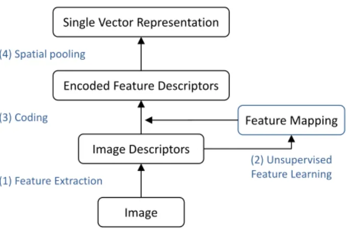
Recently, researchers have tried to improve image features for object classification via unsupervised learning. A common unsupervised feature learning framework for classification is as follows: (1) densely extract image descriptors (e.g., SIFT [88] or

(29)

Image Image Descriptors Encoded Feature Descriptors Single Vector Representation

Feature Mapping (1) Feature Extraction (2) Unsupervised Feature Learning (3) Coding (4) Spatial pooling

Figure 2.1: Pipeline for constructing features in object recognition.

HOG [22]); (2) train a feature mapping using an unsupervised learning algorithm; (3) once the feature mapping is learned, encode the descriptors to obtain “mid-level features” [15, 143]; (4) pool the single vector from multi-scaled sub-regions (e.g., spatial pyramid matching [74]) that characterize the entire image. The representations are then provided as inputs for linear or nonlinear classifiers (e.g., support vector machines). This pipeline is shown as a diagram in Figure 2.1.

Indeed, advanced encoding algorithms for image descriptors can provide significant improvements in object recognition. For example, Yang et al. [143] applied patch-based (non-convolutional) sparse coding on densely extracted SIFT descriptors to obtain sparse feature representations (ScSPM). Similarly, Wang et al. [135] proposed LLC based on locality. Boureau et al. [15] also used sparse coding, but they considered macrofeatures, which encode neighboring low-level descriptors to incorporate the spatial information. While these models arenottrained convolutionally, we use the CRBM [83]

as an unsupervised learning algorithm on top of the SIFT descriptors. Our feature representation is robust to translation variations of images and effectively captures the larger spatial context, as shown in the experiments.

Convolutional extensions of unsupervised learning algorithms, such as sparse coding and RBMs, have been successful in developing powerful image representations. For example, [148] and [60] developed algorithms for convolutional sparse coding, which

(30)

approximately solves the L1-regularized optimization problem to minimize the

recon-struction error between the data and the higher layer features convolved with the fil-ters. Our approach is different from these methods in that we used CRBM instead of convolutional sparse coding. Further, we verified the advantage of convolutional train-ing through the experimental comparison between convolutional and non-convolutional training.

Compared to sparse coding, the RBM can compute posterior probabilities in a feed-forward way, which is usually orders of magnitude faster. This computational efficiency provides a significant advantage over sparse coding since it scales up to a much larger number of codes. Furthermore, CRBMs are amenable to GPU computation resulting in another order of magnitude speedup.

2.3

Preliminaries

2.3.1 Restricted Boltzmann machines

The restricted Boltzmann machine is a bipartite, undirected graphical model with visible (observed) units and hidden (latent) units. The RBM can be understood as an MRF with latent factors that explains the input visible data using binary latent variables. The RBM consists of visible data vof dimensionL that can take real values or binary values, and stochastic binary variables h of dimensionK. The parameters of the model are the weight matrix W ∈ _RL×K that defines a potential between visible

input variables and stochastic binary variables, the biases c∈_RL for visible units, and

the biases b∈_RK _{for hidden units.}

(31)

its joint probability distribution can be defined as follows: P(v,h) = 1 Z exp(−E(v,h)), (2.1) E(v,h) = 1 2σ2 X i (vi−ci)2− 1 σ X i,j viWijhj− X j bjhj. (2.2) where Z =R v P

hexp (−E(v,h)) is a normalization constant. The conditional

distribu-tion of this model can be written as follows:

P(hj = 1|v) = exp 1 σ P iWijvi+bj P hj∈{0,1}exp 1 σ P iviWijhj+hjbj = exp 1 σ P iWijvi+bj 1 + exp 1 σ P iWijvi+bj = sigm( 1 σ X i Wijvi+bj), (2.3) P(vi|h)∝ exp   1 2σ2(vi−ci) 2 ₋ 1 σ X j viWijhj   = exp   1 2σ2(v 2 i +c 2 i −2vici−2σ X j viWijhj)   ∝ exp   1 2σ2(vi−σ X j Wijhj−ci)2  =N(v_i;σ X j Wijhj+ci, σ2). (2.4)

where sigm(s) = _1+exp(1 ₋_s₎ is the sigmoid function, and N(·;·,·) is a Gaussian

distribu-tion. Here, the variables in a layer (given the other layers) are conditionally independent, and thus we can perform block Gibbs sampling in parallel.

The RBM can be trained using sampling-based approximate maximum-likelihood, e.g., contrastive divergence (CD) approximation [44]. After training the RBM, the posterior (Equation (2.3)) of the hidden units (given input data) can be used as feature representations for classification tasks.

2.3.2 Convolutional RBMs

The Gaussian restricted Boltzmann machine is defined for input data in the form of vectors and does not model spatial context effectively. Thus, to make the RBMs

(32)

NH (= NV –ws+ 1)

NV

Visible layer Hidden layer

k=1,…,K(K=6) l=1,…,L(L=4) hk ij + ws(ws=4) vl ij Wk,l

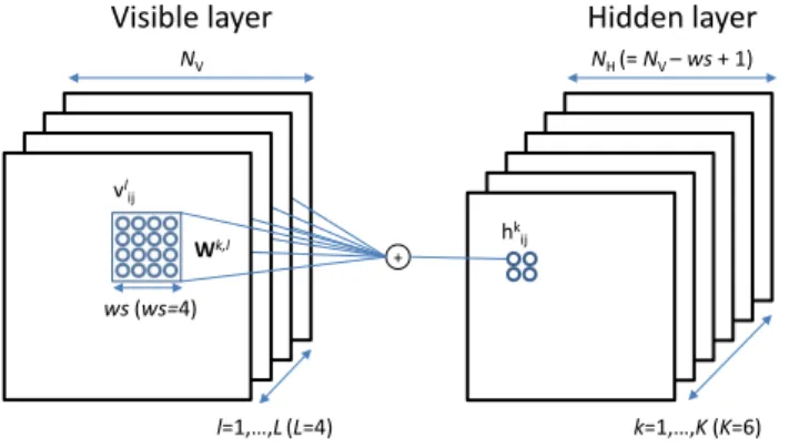
Figure 2.2: Illustration of CRBM. NV and NH refer to the size of visible and hidden

layer, and ws to the size of convolution filter. The convolutional filter for the l-th channel (of size ws×ws) corresponding to k-th hidden group is denoted as Wk,l_.

scalable to more realistic and larger images, [84] proposed the convolutional restricted Boltzmann machine (CRBM). The CRBM can be viewed as a convolutional learning algorithm that can detect salient patterns in unlabeled (image) data. A schematic description of the Gaussian CRBM is provided in Figure 2.2, whose energy function is defined as follows: E(v,h) = 1 2σ2 L X l=1 X i,j (v_i,jl −cl)2− 1 σ K X k=1 L X l=1 X i,j,r,s hk_i,jW_r,sk,lv_il₊_r₋₁_,j₊_s₋₁ − K X k=1 bk X i,j hk_i,j (2.5) = ₂1 σ2 L X l=1 X i,j (v_i,jl −cl)2− L X l=1 X i,j v_i,jl K X k=1 1 σ(W k,l_∗_hk₎ i,j ! − K X k=1 bk X i,j hk_i,j (2.6) = ₂1 σ2 L X l=1 X i,j (v_i,jl −cl)2− K X k=1 X i,j hk_i,j L X l=1 1 σ(Wf k,l_∗_vl₎ i,j+bk ! , (2.7)

wherev∈_RNV×NV×Ldenotes the visible nodes with_Lchannels,1,2 and_h ∈

RNH×NH×K denotes the hidden nodes withKgroups. The visible nodes and hidden nodes are related by the 4-d weight matrix W∈ _Rws×ws×L×K_{. More precisely,}_Wk,l _∈

Rws×ws represents

the connection between the units ink-th hidden group andl-th visible channel, and it is shared among the hidden units in the k-th group across all spatial locations. We define 1_{For the simplicity of presentation, we assume that input images are “square” shaped; however, the}

algorithm is applicable to images of arbitrary aspect ratios.

(33)

f

Wk,l _{as the 2-d filter matrix} _Wk,l _{flipped vertically and horizontally, i.e., in Matlab}

notation, Wfk,l =f liplr(f lipud(Wk,l)). The visible units in thel-th channel share the

bias cl, and the hidden units in thek-th hidden group share the bias bk.

The conditional probability of the CRBM can be written as follows:

P(hk_i,j = 1|v) = sigm X l 1 σ(Wf k,l_∗_vl₎ i,j+bk ! , (2.8) P(vl|h) =N vl;σX k Wk,l∗hk+cl, σ2I ! . (2.9)

The convolutional RBM can be trained like the standard RBM using CD. Since the CRBM is highly overcomplete, sparsity regularization [82] is used to encourage the hidden units to have sparse activations.

2.4

Efficient Training of RBMs

Although the RBM has shown promise in computer vision problems, it is not yet as commonly used as other unsupervised learning algorithms primarily because of its difficulty in training. To address this issue, we provide a novel training algorithm by exploiting the relationship between clustering methods and RBMs.

2.4.1 Equivalence between mixture models and RBMs with a softmax con-straint

In this section, we show that a Gaussian RBM with softmax hidden units can be converted into a GMM, and vice versa. This connection between mixture models and RBMs with a softmax constraint completes the chain of links between Kmeans, GMMs, Gaussian-softmax RBMs, sparse RBMs, and CRBMs. This chain of links will motivate an efficient training method for sparse RBMs and CRBMs.

(34)

Gaussian mixture model is a directed graphical model where the likelihood of visi-ble units is expressed as a convex combination of Gaussian distributions. The likelihood of a GMM with K+ 1 Gaussians can be written as follows:

P(v) =

K X

k=0

πkN(v;µk,Σk) (2.10)

For the rest of this section, we denote the GMM with shared spherical covariance as GMM(µ_k, σ2_I_{), when}_Σ

k=σ2Ifor all k∈ {0,1, . . . , K}. For the GMM with arbitrary

positive definite covariance matrices, we will use the shorthand notation GMM(µ_k,Σk).

Gaussian-softmax RBM is a Gaussian RBM with a constraint that at most one hidden unit can be activated for each input, i.e., P

jhj ≤1. The energy function of the

Gaussian-softmax RBM can be written in a vectorized form as follows:

E(v,h) = 1 2σ2kv−ck 2₋ 1 σv T_Wh₋_bT_h _{subject to} X j hj ≤1 (2.11)

The conditional probabilities can be computed as follows:

P(v|h) = N(v;σWh+c, σ2I) (2.12) P(hj = 1|v) = exp(1 σw T jv+bj) 1 +P j0exp(1 σw T j0v+b_j0) , (2.13)

where wj is thej-th column of theWmatrix, often denoted as a “basis” vector for the

j-th hidden unit. In this model, there areK+ 1 possible configurations (i.e., all hidden units are 0, or only one hidden unit hj is 1 for some j).

Equivalence between GMMs and Gaussian-softmax RBMs. The conditional probability of visible units given the hidden unit activations of Gaussian-softmax RBM follows a Gaussian distribution, as seen in Equation (2.12). From this perspective, the Gaussian-softmax RBM can be viewed as a mixture of Gaussians whose mean

(35)

components correspond to possible hidden unit configurations.3 _{In this section, we}

show an explicit equivalence between these two models by formulating the conversion equations between GMM(µ_k, σ2_I_{) with} _K_{+ 1 Gaussian components and the}

Gaussian-softmax RBM with K hidden units.

Proposition II.1. The mixture of K + 1 Gaussians with shared spherical covariance of σ2I is equivalent to the Gaussian-softmax RBM with K hidden units.

Proof. We prove by constructing the following conversions.

(1) From Gaussian-softmax RBM to GMM(µ_k, σ2_I): _{We begin by the}

decompo-sition using a chain rule:

P(v,h) =P(v|h)P(h), where P(h) = 1 Z Z dvexp(−E(v,h)).

Since there are only a finite number of hidden unit configurations, we can explicitly enumerate the prior probabilities:

P(hj = 1) = R dvexp(−E(v, hj = 1)) P j0R dvexp(−E(v, h_j0 = 1)) If we define ˜πj = R

dvexp(−E(v, hj = 1)), then we have P(hj = 1) =

˜

πj

P

j0π˜j0 ,πj. In fact, ˜πj can be analytically calculated as follows:

˜ πj = Z dvexp(−E(v, hj = 1)) = Z dvexp(− 1 2σ2kv−ck 2₊ 1 σv T_w j +bj) = (√2πσ)Lexp(bj + 1 2kwjk2+ 1 σc T_w j)

3_{In fact, the Gaussian RBM (without any constraints) can be viewed as a mixture of Gaussians with}

an exponential number of components. However, it is nontrivial to use this notion itself to develop a useful algorithm.

(36)

Using this definition, we can show the following equality:

P(v) = X

j

πjN(v;σwj+c, σ2I).

(2) From GMM(µ_k, σ2_{I) to Gaussian-softmax RBM:} _{We will also show this by}

construction. Suppose we have the following GMM with K + 1 components and the shared spherical covariance σ2_I:

P(v) = K X j=0 πjN(v;µj, σ 2_I₎_. _(2.14)

We can convert from this GMM(µ_k, σ2_I_{) to a Gaussian-softmax RBM using the}

follow-ing transformations: c=µ₀ wj = 1 σ(µj −c), j = 1, ..., K bj = log πj π0 −1 2kwjk2− 1 σw T jc. (2.15)

It is easy to see that the conditional distribution P(v|hj = 1) can be formulated as

a Gaussian distribution with mean µ_j = σwj +c, which is identical to that of the

Gaussian-softmax RBM. Further, we can recover the posterior probability of hidden units given the visible units as follows:

P(hj = 1|v) = πjexp(−₂1_σ2kv−σwj −ck2) PK j0₌₀π_j0exp(− 1 2σ2kv−σwj0−ck2) = exp( 1 σw T jv+bj) 1 +PK j0₌₁exp(1 σw T j0v+b_j0)

Therefore, a GMM can be converted to Gaussian RBM with a softmax constraint. Similarly, the GMM with shared diagonal covariance is equivalent to the Gaussian-softmax RBM with a slightly more general energy function, where each visible unit v

(37)

has its own noise parameter σi, as stated below.

Corollary II.2. The mixture of K + 1 Gaussians with a shared diagonal covariance matrix (with diagonal entries σ_i2, i = 1, ..., L) is equivalent to the Gaussian-softmax RBM with the following energy function: E(v,h) =P

i ₂_σ12

i(

vi−ci)2−Pi,j _σ1_iviWijhj − P

jbjhj.

Further, the equivalence between mixture models and RBMs can be shown for other settings. For example, the following corollaries can be derived from Proposition II.1. Corollary II.3. The binary RBM (i.e., when the visible units are binary) with a softmax constraint on hidden units and the mixture of Bernoulli models are equivalent.

Corollary II.4. GMM(0,Σk) with arbitrary covariance matrices and the factored

3-way RBM [104] with a softmax constraint on hidden units are equivalent.

We provide proofs for Corollary II.3 and II.4 in Appendix A.

Implication. Proposition II.1 has important ramifications. First, it is well known that K-means can be viewed as an approximation of a GMM with spherical covariance by letting σ→0 [12]. Compared to GMMs, the training of K-means is highly efficient;

therefore, it is plausible to train K-means to provide an initialization of a GMM.4 Then,

the GMM is trained with expectation-maximization (EM) algorithm, and we convert it to an RBM with softmax units. As will be discussed, this provides an efficient initialization for training sparse RBMs and CRBMs.

2.4.2 Activation constrained RBMs, sparse RBMs, and convolutional RBMs We extend the Gaussian-softmax RBM to more general Gaussian RBMs that allow at most α≥1 hidden units to be active for a given input example. We call this model

4_{K-means learns cluster centroids and provides hard-assignment of training examples to the cluster}

centroids (i.e., each example is assigned to one centroid). This hard-assignment can be used to initialize GMM’s parameters, such asπ andσ, by running one M-step in the EM algorithm.

(38)

the activation constrained RBM, and its energy function is written as follows: E(v,h) = 1 2σ2kv−ck 2₋ 1 σv T_Wh₋_bT_h _{subject to} X j hj ≤α (2.16)

Note that the number of possible hidden configurations grows polynomial with α.5

Therefore, such relaxation provides more expressive power than GMMs. However, there is a trade-off between the expressive power (or capacity), and the tractability of exact inference and maximum-likelihood training. For example, an exact EM algorithm will require polynomial time complexity ofO(Kα), which may be computationally expensive. To address such difficulties, we approximate the activation constrained RBM to the sparse RBM [82]. Specifically, the sparse RBM is a variant of the RBM trained with a regularizer that encourages the average activation to be low (i.e., with target sparsityp0)

in the hidden representations. By setting p0 =α/K, the sparse RBM can be regarded

as an approximation to the activation constrained RBM with a constraint P

jhj ≤α.

The inference and training of sparse RBMs is much more efficient as α increases. We further observe that the CRBM is a generalization of the sparse RBM. Specifi-cally, the two algorithms are equivalent when (1) the filter size of the CRBM is 1 (i.e., the convolution does not smooth the image); or (2) the filter size is the same as the image size (i.e., this is essentially equivalent to vectorizing the whole image, which is usually not interesting). For example, note that non-convolutional feature learning al-gorithms (e.g., sparse RBM) on SIFT descriptors would have a weight matrix of size 128×K, which is equivalent to that of convolutional algorithms (1×1×128×K, i.e., no interactions between adjacent hidden units). In general, CRBMs can model a larger spatial context using ws×ws×L as weights for each hidden unit.

Predictions. Based on the connections described, we make the following predictions: 5_If _α_{→ ∞} _{or there is no such constraint, the model is equivalent to the Gaussian RBM that has}

(39)

Algorithm 1 Efficient training algorithm for sparse or convolutional RBMs

1: Train K+ 1 centroids µ_k via K-means.

2: Initialize GMM(µ_k, σ2_I_{) parameters from K-means.}

3: Train GMM(µ_k, σ2_I) via EM.

4: Initialize the RBM parameters (see Proposition II.1). 5: Train sparse or convolutional RBMs (e.g., via CD).

• K-means, GMM, and Gaussian-softmax RBM (with the same K) should have similar expressive power and show similar classification performance.

• When α > 1, sparse RBMs can give better classification performance than K-means or GMMs due to their increased expressive power.

• When convolutional filter size is larger than 1, CRBMs can give better classi-fication performance than non-convolutional RBMs since they can learn spatial context more efficiently.

These predictions will be verified with our efficient training method in the following section.

2.4.3 Algorithm and implementation details

The overall procedure for training sparse or convolutional RBMs is shown in Algo-rithm 1. In addition, we used the following methods to select hyperparameters.

Setting the σ automatically. As in Equation (2.4),σ roughly controls the noise in the visible units. Typically, σ is fixed during training and treated as a hyperparameter that needs to be cross-validated. As an alternative, we used the following heuristic to automatically tune the σ value. Suppose that we are given a fixed set of hidden unit values ˆh, then we have the following conditional probability distribution for the Gaussian RBM:

(40)

If we apply the maximum likelihood estimation of σgiven ˆh fixed, thenσshould be the sample standard deviation of v−(σWhˆ+c). Here, we use ˆh as the expectation ofh given input v. Thus, we update σ so that it becomes close to the reconstruction error of the training data.6 The same method also applies to convolutional training.

Setting the L2 regularization. When training RBMs, a hyperparameter for L2

regularization (that penalizes high L2 norm of W) typically has to be determined via

cross validation. However, due to the connections between mixture models and RBMs discussed in section 2.4.1, setting the L2 regularization is straightforward. Specifically,

the clustering-based initialization justifies using the L2 regularization hyperparameter

obtained from clustering models, which are often very small. In our experiments, we used 0.0001 without tuning.

In the following section, we show the efficacy of our training algorithm and provide experimental evidence for the above predictions. From the experiments, we find that a combination of moderately sparse (1 < α K) representations with a moderate amount of spatial convolution (1 < wsNV) performs the best for object recognition.

Further, we show that our feature representation achieves state-of-the-art performance.

2.5

Experiments and Discussions

In this section, we report classification results based on two datasets: Caltech 101 [32] and Caltech 256 [37]. In the experiments, we used SIFT as low-level de-scriptors, which were extracted densely from every 6 pixels with a patch size of 24. We resized the images to no larger than 300×300 pixels with a preserved aspect ratio for

computational efficiency. After training the codebook, feature vectors were pooled from the 4×4, 2×2, and 1×1 subregions using max-pooling and then concatenated to single

6_{We define the reconstruction error as} q 1

LM

PM

i=1kv(i)−(σWhˆ(i)+c)k2 for training examples

(41)

training images 5 10 15 20 25 30 Lazebnik et al. [74] - - 56.4 - - 64.6 Griffin et al. [37] 44.2 54.5 59.0 63.3 65.8 67.6 Yang et al. [143] - - 67.0 - - 73.2 Wang et al. [135] 51.2 59.8 65.4 67.7 70.2 73.4 Boureau et al. [15] - - - 75.7 K-means (K=4096) 47.6 58.1 63.4 66.6 69.1 70.9 GMM (K=4096) 50.2 60.3 65.3 68.6 70.8 72.2 sparse RBM (K=4096) 54.2 64.0 68.6 71.2 73.1 74.9 CRBM (K=2048) 56.5 66.4 70.7 73.5 75.4 77.4 CRBM (K=4096) 56.7 66.7 71.3 74.2 76.2 77.8 Table 2.1: Average test classification accuracy for Caltech 101.

feature vectors. We used linear SVM [30] for classifier on randomly selected training images (with a fixed number of images per class) and then evaluated the classification accuracy on the rest of the images. We performed 5-fold cross-validation to determine hyperparameters on each randomly selected training set and reported the test accuracy averaged over 10 trials.

2.5.1 Caltech 101

The Caltech 101 dataset [32] is composed of 9,144 images split into 101 object categories, such as vehicles, artifacts, and animals, as well as one background category with significant variances in shape. The number of images in each class varies from 31 to 800. For fair comparisons, we performed experiments as in other studies [32, 143, 135]. Specifically, for each trial, we randomly selected 5,10, . . . ,30 images from each class, including the background class, and trained a linear classifier. The remaining images from each class were tested, and the average accuracy over the classes was reported.

We summarize the results from our proposed method and other existing methods in Table 2.1. Our algorithm clearly outperformed other state-of-the-art algorithms using a single type of feature. Specifically, our method breaks the record on the Caltech 101 dataset by 4.3% for 15 training images and 2.1% for 30 training images.

(42)

training images 15 30 45 60 Griffin et al. [37] 28.30 34.10 - -van Gemert et al. [129] - 27.17 -

-Yang et al. [143] 27.73 34.02 37.46 40.14 Wang et al. [135] 34.36 41.19 45.31 47.68 CRBM (K=4096) 35.09 42.05 45.69 47.94 Table 2.2: Average test classification accuracy for Caltech 256. 2.5.2 Caltech 256

We also tested our algorithm on a more challenging dataset. Caltech 256 dataset [37] is composed of 30,607 images split into 256 object categories with more variability and finer classifications, as well as one “clutter” class of random pictures. Each class contains at least 80 images; the objects in each image are more variant in size, location, pose, etc., than those of Caltech 101 dataset. We followed the standard experimental settings from the benchmarks [37, 143], and the overall classification accuracy was averaged over 10 random trials. The summary of the results is reported in Table 2.2. Our algorithm performed slightly better than the LLC [135] algorithm, with considerably large margins to many other methods on Caltech 256 dataset.

2.5.3 Analysis of hyperparameters

To provide a better understanding of our proposed algorithm, we give a detailed analysis of the hyperparameters: sparsity and convolutional filter size. We performed the control experiments on Caltech 101 dataset while fixing the number of bases to 1024. In most cases, we observed improvement as the number of hidden bases increased, which is consistent with what others have reported [21]. All results reported in this section are validation accuracy (5-fold cross validation on the training set).

Sparsity (α/K). The performance of sparse models, such as sparse coding and sparse RBMs, can vary significantly as a function of sparsity level. As we discussed in

(43)

Sec-tion 2.4, the sparse RBM can be more expressive than K-means or GMMs. While K-means and GMM have sparsity of 1/K on average (i.e., allow only one cluster to be active for a given input), the sparse RBM can control sparsity by setting the target sparsity value p0 =α/K.

In this experiment, we compared two settings for sparse RBM training—one by initializing from GMM as described in Section 2.4, and the other by initializing randomly (baseline). Figure 2.3 (left) shows the average validation accuracy as a function of sparsity (α/K). Compared to the K-means and GMM, the sparse RBM with random initialization performed very poorly in the low α regime (i.e., when its corresponding number of activation is roughly 1). However, by using an efficient training method described in Section 2.4, the sparse RBM performs as well as K-means and GMM when the target sparsity is close to 1/K, and significantly outperforms K-means and GMM when the representation is less sparse. Overall, the effect of accurate initialization is striking, especially in the high sparsity regime, and the best validation accuracy (maximum over α) was improved by 2% for both 15 and 30 training images.

Convolution filter size. Convolutional learning is powerful since it captures the spatial correlation between neighboring descriptors (e.g., pixels or dense SIFT) more efficiently than non-convolutional learning. The size of the filter, however, should be selected carefully. For instance, it is difficult to capture enough spatial information with small size filters; on the other hand, overly large filter size can result in severe over-smoothing of small details in the image. Therefore, we investigate how the filter size affects the performance.

In this experiment, we fixed the number of bases (K = 1024) and spa