DRINet for medical image segmentation

DRINet for Medical Image Segmentation

Liang Chen, Paul Bentley, Kensaku Mori, Kazunari Misawa, Michitaka Fujiwara, Daniel Rueckert

Fellow IEEE

Lorem ipsum dolor sit amet, consectetuer adipiscing elit. Ut purus elit, vestibulum ut, placerat ac, adipiscing vitae, felis. Curabitur dictum gravida mauris. Nam arcu libero, nonummy eget, consectetuer id, vulputate a, magna. Donec vehicula augue eu neque. Pellentesque habitant morbi tristique senectus et netus et malesuada fames ac turpis egestas. Mauris ut leo. Cras viverra metus rhoncus sem. Nulla et lectus vestibulum urna fringilla ultrices. Phasellus eu tellus sit amet tortor gravida placerat. Integer sapien est, iaculis in, pretium quis, viverra ac, nunc. Praesent eget sem vel leo ultrices bibendum. Aenean faucibus. Morbi dolor nulla, malesuada eu, pulvinar at, mollis ac, nulla. Curabitur auctor semper nulla. Donec varius orci eget risus. Duis nibh mi, congue eu, accumsan eleifend, sagittis quis, diam. Duis eget orci sit amet orci dignissim rutrum.

Nam dui ligula, fringilla a, euismod sodales, sollicitudin vel, wisi. Morbi auctor lorem non justo. Nam lacus libero, pretium at, lobortis vitae, ultricies et, tellus. Donec aliquet, tortor sed accumsan bibendum, erat ligula aliquet magna, vitae ornare odio metus a mi. Morbi ac orci et nisl hendrerit mollis. Suspendisse ut massa. Cras nec ante. Pellentesque a nulla. Cum sociis natoque penatibus et magnis dis parturient montes, nascetur ridiculus mus. Aliquam tincidunt urna. Nulla ullam-corper vestibulum turpis. Pellentesque cursus luctus mauris.

Nulla malesuada porttitor diam. Donec felis erat, congue non, volutpat at, tincidunt tristique, libero. Vivamus viverra fermentum felis. Donec nonummy pellentesque ante. Phasellus adipiscing semper elit. Proin fermentum massa ac quam. Sed diam turpis, molestie vitae, placerat a, molestie nec, leo. Maecenas lacinia. Nam ipsum ligula, eleifend at, accumsan nec, suscipit a, ipsum. Morbi blandit ligula feugiat magna. Nunc eleifend consequat lorem. Sed lacinia nulla vitae enim. Pellentesque tincidunt purus vel magna. Integer non enim. Praesent euismod nunc eu purus. Donec bibendum quam in tellus. Nullam cursus pulvinar lectus. Donec et mi. Nam vulputate metus eu enim. Vestibulum pellentesque felis eu massa.

Quisque ullamcorper placerat ipsum. Cras nibh. Morbi vel justo vitae lacus tincidunt ultrices. Lorem ipsum dolor sit amet, consectetuer adipiscing elit. In hac habitasse platea dictumst. L. Chen is with the Department of Computing and the Division of Brain Sciences, Department of Medicine, Imperial College London, UK, SW7 2AZ, e-mail: [email protected].

P. Bentley is with the Division of Brain Sciences, Department of Medicine, Imperial College London.

K. Mori is with Graduate School of Informatics, Nagoya University. K. Misawa is with Aichi Cancer Center.

M. Fujiwara is with Nagoya University Hospital.

D. Rueckert is with the Department of Computing, Imperial College London.

Integer tempus convallis augue. Etiam facilisis. Nunc elemen-tum fermenelemen-tum wisi. Aenean placerat. Ut imperdiet, enim sed gravida sollicitudin, felis odio placerat quam, ac pulvinar elit purus eget enim. Nunc vitae tortor. Proin tempus nibh sit amet nisl. Vivamus quis tortor vitae risus porta vehicula.

Fusce mauris. Vestibulum luctus nibh at lectus. Sed biben-dum, nulla a faucibus semper, leo velit ultricies tellus, ac venenatis arcu wisi vel nisl. Vestibulum diam. Aliquam pellen-tesque, augue quis sagittis posuere, turpis lacus congue quam, in hendrerit risus eros eget felis. Maecenas eget erat in sapien mattis porttitor. Vestibulum porttitor. Nulla facilisi. Sed a turpis eu lacus commodo facilisis. Morbi fringilla, wisi in dignissim interdum, justo lectus sagittis dui, et vehicula libero dui cursus dui. Mauris tempor ligula sed lacus. Duis cursus enim ut augue. Cras ac magna. Cras nulla. Nulla egestas. Curabitur a leo. Quisque egestas wisi eget nunc. Nam feugiat lacus vel est. Curabitur consectetuer.

Suspendisse vel felis. Ut lorem lorem, interdum eu, tincidunt sit amet, laoreet vitae, arcu. Aenean faucibus pede eu ante. Praesent enim elit, rutrum at, molestie non, nonummy vel, nisl. Ut lectus eros, malesuada sit amet, fermentum eu, sodales cursus, magna. Donec eu purus. Quisque vehicula, urna sed ul-tricies auctor, pede lorem egestas dui, et convallis elit erat sed nulla. Donec luctus. Curabitur et nunc. Aliquam dolor odio, commodo pretium, ultricies non, pharetra in, velit. Integer arcu est, nonummy in, fermentum faucibus, egestas vel, odio.

Sed commodo posuere pede. Mauris ut est. Ut quis purus. Sed ac odio. Sed vehicula hendrerit sem. Duis non odio. Morbi ut dui. Sed accumsan risus eget odio. In hac habitasse platea dictumst. Pellentesque non elit. Fusce sed justo eu urna porta tincidunt. Mauris felis odio, sollicitudin sed, volutpat a, ornare ac, erat. Morbi quis dolor. Donec pellentesque, erat ac sagittis semper, nunc dui lobortis purus, quis congue purus metus ultricies tellus. Proin et quam. Class aptent taciti sociosqu ad litora torquent per conubia nostra, per inceptos hymenaeos. Praesent sapien turpis, fermentum vel, eleifend faucibus, vehicula eu, lacus.

Pellentesque habitant morbi tristique senectus et netus et malesuada fames ac turpis egestas. Donec odio elit, dictum in, hendrerit sit amet, egestas sed, leo. Praesent feugiat sapien aliquet odio. Integer vitae justo. Aliquam vestibulum fringilla lorem. Sed neque lectus, consectetuer at, consectetuer sed, eleifend ac, lectus. Nulla facilisi. Pellentesque eget lectus. Proin eu metus. Sed porttitor. In hac habitasse platea dictumst. Suspendisse eu lectus. Ut mi mi, lacinia sit amet, placerat et, mollis vitae, dui. Sed ante tellus, tristique ut, iaculis eu, malesuada ac, dui. Mauris nibh leo, facilisis non, adipiscing quis, ultrices a, dui.

Copyright c2017 IEEE. Personal use of this material is permitted. However, permission to use this material for any other purposes must be obtained from the IEEE by sending a request to [email protected].

Morbi luctus, wisi viverra faucibus pretium, nibh est plac-erat odio, nec commodo wisi enim eget quam. Quisque libero justo, consectetuer a, feugiat vitae, porttitor eu, libero. Sus-pendisse sed mauris vitae elit sollicitudin malesuada. Maece-nas ultricies eros sit amet ante. Ut venenatis velit. MaeceMaece-nas sed mi eget dui varius euismod. Phasellus aliquet volutpat odio. Vestibulum ante ipsum primis in faucibus orci luctus et ultrices posuere cubilia Curae; Pellentesque sit amet pede ac sem eleifend consectetuer. Nullam elementum, urna vel imperdiet sodales, elit ipsum pharetra ligula, ac pretium ante justo a nulla. Curabitur tristique arcu eu metus. Vestibulum lectus. Proin mauris. Proin eu nunc eu urna hendrerit faucibus. Aliquam auctor, pede consequat laoreet varius, eros tellus scelerisque quam, pellentesque hendrerit ipsum dolor sed augue. Nulla nec lacus.

Suspendisse vitae elit. Aliquam arcu neque, ornare in, ullamcorper quis, commodo eu, libero. Fusce sagittis erat at erat tristique mollis. Maecenas sapien libero, molestie et, lobortis in, sodales eget, dui. Morbi ultrices rutrum lorem. Nam elementum ullamcorper leo. Morbi dui. Aliquam sagittis. Nunc placerat. Pellentesque tristique sodales est. Maecenas imperdiet lacinia velit. Cras non urna. Morbi eros pede, suscipit ac, varius vel, egestas non, eros. Praesent malesuada, diam id pretium elementum, eros sem dictum tortor, vel consectetuer odio sem sed wisi.

Sed feugiat. Cum sociis natoque penatibus et magnis dis parturient montes, nascetur ridiculus mus. Ut pellentesque au-gue sed urna. Vestibulum diam eros, fringilla et, consectetuer eu, nonummy id, sapien. Nullam at lectus. In sagittis ultri-ces mauris. Curabitur malesuada erat sit amet massa. Fusce blandit. Aliquam erat volutpat. Aliquam euismod. Aenean vel lectus. Nunc imperdiet justo nec dolor.

Etiam euismod. Fusce facilisis lacinia dui. Suspendisse potenti. In mi erat, cursus id, nonummy sed, ullamcorper eget, sapien. Praesent pretium, magna in eleifend egestas, pede pede pretium lorem, quis consectetuer tortor sapien facilisis magna. Mauris quis magna varius nulla scelerisque imperdiet. Aliquam non quam. Aliquam porttitor quam a lacus. Praesent vel arcu ut tortor cursus volutpat. In vitae pede quis diam bibendum placerat. Fusce elementum convallis neque. Sed dolor orci, scelerisque ac, dapibus nec, ultricies ut, mi. Duis nec dui quis leo sagittis commodo.

Abstract—Convolutional neural networks (CNNs) have revolu-tionized medical image analysis over the past few years. The U-Net architecture is one of the most well-known CNN architectures for semantic segmentation and has achieved remarkable successes in many different medical image segmentation applications. The U-Net architecture consists of standard convolution layers, pooling layers, and upsampling layers. These convolution layers learn representative features of input images and construct seg-mentations based on the features. However, the features learned by standard convolution layers are not distinctive when the differ-ences among different categories are subtle in terms of intensity, location, shape, and size. In this paper, we propose a novel CNN architecture, called Dense-Res-Inception Net (DRINet), which addresses this challenging problem. The proposed DRINet consists of three blocks, namely a convolutional block with dense connections, a deconvolutional block with residual Inception modules, and an unpooling block. Our proposed architecture outperforms the U-Net in three different challenging applications, namely multi-class segmentation of cerebrospinal fluid (CSF) on

brain CT images, multi-organ segmentation on abdominal CT images, multi-class brain tumour segmentation on MR images.

Index Terms—Convolutional neural network, medical image segmentation, brain atrophy, abdominal organ segmentation.

I. INTRODUCTION

Significant progress has been achieved in the field of medical image analysis in recent years due to the advent of CNNs [1]. Within medical imaging, the problem of im-age segmentation has been one of the major challenges. Segmentation is a pre-requisite for many different types of clinical applications, including brain segmentation [2], cardiac ventricle segmentation [3], abdominal organ segmentation [4], and cell segmentation in biological images [5]. In these applications, the results of the segmentation are usually used to derive quantitative measurements or biomarkers for subsequent diagnosis and treatment planning.

Among the different approaches that use CNNs for medical image segmentation, the U-Net architecture [5] and its 3D extension [6] are widely used because of their flexible architec-tures. In the first part of the U-Net architecture (analysis path), deep features are learned while the second part of the U-Net architecture (synthesis path) performs segmentation based on these learned features. Training the two parts of the network in an end-to-end fashion yields good segmentation results. As the number of features in the first part of network is reduced because of convolutions and poolings, skip connections are used to allow dense feature maps from the analysis path to propagate to the corresponding layers in the synthesis part of the network, which improves the performance significantly.

However, the limitation of the U-Net architecture is its scal-ability. Specifically, deeper networks learn more representative features and result in better performance. Adding more layers to the network enlarges the parameter space, which allows the network to learn more representative features. However, this also increases the difficulties in training the network because gradients are likely to vanish during training. Therefore, the challenge is to make the network wider and deeper without gradient vanishing.

In computer vision, the state-of-the-art CNN architec-tures include the densely connected convolutional network (DenseNet) [7], [8] and the Inception-ResNet [9]. The DenseNet approach consists of a number of dense blocks with pooling layers between them to reduce the size of the feature maps. Within each dense block, layers are directly connected with all of their preceding layers, which is implemented via concatenation of feature maps in subsequent layers. This dense architecture has a number of advantages: Firstly, the concatenation of feature maps enables deep supervision so that gradients are propagated more easily to preceding layers, which makes the network training easier. Secondly, bottleneck layers (convolution layers with 1-by-1 kernels) are used to control the growth rate of parameters in the network. Finally, in the DenseNet architecture the final classifier uses features from all layers (instead of only features from the last layer as in standard CNN approaches), leading to improved classification performance.

The Inception network [10] is a CNN architecture which uses the Inception modules and allows for very deep net-works. The main purpose of the Inception modules are: 1) to increase the depth and width of networks without adding more parameters; and 2) to achieve multi-scale features for processing. These are achieved by carefully designing struc-tures of the Inception modules. The latest version of the Inception architecture [9] also uses residual connections, i.e. ResNet. Fig. 1 shows an overview of the Inception-ResNet: a stem convolution block, stacks of inception and reduction blocks, and the classifier. The stem block consists of a number of standard convolution and pooling layers, reducing the size of feature maps in lower layers (the ones close to the input). This aims to be memory efficient in training but is not strictly necessary. Each inception block consists of number of inception modules. The reduction blocks are inception modules with dimension reduction. An inception module consists of a number of branches of convolution layers. In each branch, a bottleneck layer reduces the number of feature maps. The feature maps are then processed by convolution layers with different sizes of kernels in different branches. The output of all branches are finally aggregated as the output of the inception module.

Fig. 1. The overall schema of the Inception-ResNet [9]. The whole architec-ture consists of some Inception and Reduction blocks. Each block contains a number of modules. The detailed structures in different blocks vary slightly. Inspired by the DenseNet and the Inception-ResNet, we propose an architecture consisting of dense connection blocks, residual Inception blocks, and unpooling blocks. We term this architecture Dense-Res-Inception Net (DRINet). We apply the proposed DRINet architecture for three challenging clinical segmentation problems, namely multi-class segmentation of brain CSF in CT images, abdominal multi-organ segmenta-tion in CT images, and brain tumour segmentasegmenta-tion (BraTS) in multi-modal MR images. The former two problems are based on clinical datasets while the last one is based on a publically benchmark dataset. Our main contributions are: 1) a novel combination of the dense connections with the inception structure to address segmentation problems. The use of dense connection blocks, residual inception blocks, and the unpooling blocks achieve high performance while maintaining computational efficiency; 2) easy and flexible implementation of the proposed network architecture; 3) state-of-the-art segmentation performance for challenging image segmentation tasks.

II. RELATED WORK

The basic CNN architecture for many semantic segmenta-tion problems is the fully convolusegmenta-tional network (FCN), shown

in Fig. 2(a), which consists of cascaded convolution, pooling, and deconvolution layers. Convolution and pooling layers form the analysis path while the convolution and deconvolution layers form the synthesis path. The analysis path and the synthesis path are usually symmetric.

The U-Net (Fig. 2(b)) is the FCN with skip layers between layers in analysis path and synthesis path. The skip layers are implemented via concatenations and they allow deep supervision for the network. As such, the errors can propagate easily through the network. Therefore, the skip layers improve the network performance. In addition, residual connections can be used in the U-Net, which results in the Res-U-Net (Fig. 2(c)). In the Res-U-Net, the residual learning is implemented using the bottleneck building blocks with residual connections, which were used in the ResNet-50/101/152 architectures [11]. The DeepLab approach [12] involved atrous convolutions and poolings within the CNN architecture to solve segmenta-tion problems, as well as condisegmenta-tional random field (CRF) mod-els for post processing. Based on the DeepLab architecture, Chen et al. [13] proposed the latest DeepLabV3 architecture. In DeepLabV3, a simple synthesis path is used. This synthesis path only consists of very few convolution layers, which is different from the synthesis path used in the FCN and the U-Net architectures. Skip connections are used to connect the analysis path and the synthesis path.

The DenseNet was extended in a fully convolutional fashion so that it can be used for segmentation tasks [14]. Specifically, an upsampling transition module was proposed in correspon-dence to the downsampling transition module in the original DenseNet. In addition, the macro-architecture of the fully convolutional DenseNet is similar to the U-Net where skip connections are used.

Finally, the Pyramid Scene Parsing Network (PSPNet) [15] was proposed to solve the challenging scene parsing problem. In the scene parsing problem, prior knowledge could be incorporated in CNNs to improve performance. For example, cars are likely to be on the road while they should not be in the sky. Global context is required to incorporate these priors. The pyramid pooling module in the PSPNet investigate features in multiple levels, achieving the state-of-the-art performance.

III. DRINET

A. Overview

Fig. 2(d) demonstrates our proposed DRINet architecture. Similar to the FCN, the DRINet has an analysis path and a synthesis path. Stacks of dense connection blocks, instead of standard convolution layers make up the analysis path, which is inspired by the DenseNet. The synthesis path consists of residual inception blocks and unpooling blocks, which are inspired by the Res-Inception Net. To be more efficient in terms of memory, the DRINet has no skip connections.

B. Dense connection block

We employ convolutional dense connection blocks [7] in the analysis path, which are shown in Fig. 3. Formally, let us assume xl is the output of the lth layer and f(·)

Fig. 2. Overview of the FCN, the U-Net, the Res-U-Net and the DRINet. DC block and RI block represent the dense connection block and the residual Inception block. In the DRINet, the DC, RI, and unpooling blocks are depicted in Fig. 3, 4, and 5, respectively. In the Res-U-Net, the residual convolution means the bottleneck building block used in the ResNet-50/101/152 [11].

Fig. 3. A dense connection block containsmconvolution layers. The output channel number of each convolution layerkiis the growth rate. BN and ReLU apply on every convolution layer. The input and output of a convolution layer is concatenated so deep supervision is allowed.

(BN) [16] and rectified linear unit (ReLU). In the standard convolution layer, we have:

xl+1=f(xl) (1)

while in the dense connection block [7] we have

xl+1 =f(xl)◦xl. (2)

Here ◦indicates concatenation.

The number of output channels from standard convolution layers are usually fixed and typically 64 or 128. As a result, it is expensive in terms of memory to concatenate the outputs of preceding convolution layers. In addition, the concatenation also leads to many redundant features. Therefore, Huang et al. [7] propose to use1×1convolutions to reduce the output size. As shown in Fig. 3, within a dense connection block, the size of the output channel for each convolution layerkiis typically

small, e.g. 12 or 24 and this is commonly referred to as the growth rate of the network.

Using dense connection blocks in the analysis path leads to three major advantages: 1) Gradient propagation through

the network is more efficient. Conventionally, it is difficult to ensure that gradients backpropagate to lower layers in the network. Therefore, it is important to use dense connection blocks to alleviate the effect of vanishing gradients. 2) The input to the synthesis path consists of feature maps output from all preceding layers, instead of only the last layer, which reuses the feature maps. 3) It is easy to use the growth rate to control the parameter space, resulting in good network performance. The latter two advantages will be verified in the following experiments.

C. Residual Inception block

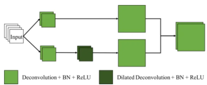
In the synthesis path of the DRINet, we propose to use the residual Inception blocks, which is depicted in Fig. 4. Similar to the original inception modules [10], the idea is to aggregate feature maps from different branches, where the input feature maps are convolved using kernels in different sizes. The residual connections make the learning easier since a residual inception block learns a function with reference to

Fig. 4. A residual Inception block is an Inception module with residual connections. An Inception module is a weighted combination of features maps from a few branches. Each branch process the input feature maps using deconvolutions with different kernel sizes.

the input feature maps, instead of learning an unreferenced function.

In terms of the kernel sizes in convolutions, it is difficult to determine the optimal size for each convolution. In the FCN and the U-Net, the kernel size of convolutions is fixed as3×3. In the inception module, convolutions of different kernel sizes are used in parallel. In implementation, the feature maps are combined using concatenation and a deconvolution layer with

1×1 kernel learns the combination weights. The deconvolu-tions are transposed convoludeconvolu-tions. In the proposed Inception modules, deconvolutions work the same as the convolutions. The purpose of this is to differentiate with convolutions in the analysis path in symbols.

Unlike the Inception Res-Net [9] having various inception modules, we propose to use identical inception blocks in the DRINet, which is easy to implement. We propose to aggregate feature maps convolved by three kernels, namely1×1,3×3, and 5×5. Inspired by the DeepLab [17], the deconvolution with a5×5kernel is replaced by a dilated deconvolution with a

3×3kernel, which is more efficient in memory. To further limit the size of the parameter space, a bottleneck deconvolution is used in each branch.

Formally, letg(·)denotes a deconvolution function followed by BN and ReLU andgb(·)andgd(·)represent bottleneck and

dilated deconvolution respectively. As a result we obtain

xl+1=gb(gb(xl)◦g(gb(xl))◦gd(gb(xl))) +xl. (3)

D. Unpooling block

Fig. 5. An unpooling block is a mini Inception module and it upsamples the input feature maps.

We propose an unpooling block shown in Fig. 5 to upsample the feature maps in the synthesis path. The unpooling block

can be viewed as a mini inception module, which combines upsampled feature maps from two branches. In each branch, the input feature maps are convolved using kernels in different sizes, namely 1×1 and 5×5. The resulting feature maps are then upsampled using a deconvolution layer with stride 2. Again, the deconvolution with a 5×5 kernel is replaced by a dilated deconvolution with a 3 × 3 kernel in order to ensure memory efficiency. Also, to limit the parameter space, the input feature maps are firstly convolved by a bottleneck layer in each branch, which is similar to the residual inception block. The combination of upsampled feature maps is achieved via concatenation. Formally, let g2(·)denotes the deconvolution function with stride 2. The upsampled feature maps are therefore:

xl+1=g2(gb(xl))◦g2(gd(gb(xl))). (4)

The major advantage of the proposed unpooling block is the aggragation of different upsampled feature maps. Specifically, simply upsampling the input feature maps using a deconvo-lution layer is likely to produce errors. For instance, a small error in the input feature maps is likely to be enlarged, which finally results in errors in the segmentation results. In contrast, convolving the input feature maps with different kernels leads to different intermediate feature maps. Upsampling these fea-ture maps separately and combining them together reduce the effect of errors.

E. Evaluation metrics

In multi-class segmentation on brain CSF and abdominal organs, we use the well-known Dice coefficient as well as sen-sitivity (SE) and precision (PR) for evaluation. In evaluation in the BraTS challenge, we use the same metrics used in the challenge, namely the Dice coefficient, the SE, the specificity (SP), and the Hausdorff95 distance. The Hausdorff95 distance is a robust version of the standard Hausdorff distance, which measures 95 quantile of the distance between two surfaces, instead of the maximum.

F. Implementation details

In this work, we use cross-entropy as the loss function for all networks. We use the Adam method [18] for optimization with the following parameters: β1= 0.9, β2 = 0.999, = 1e−8. An initial learning rate of1e−3is utilized. The weights are all initialised from a truncated normal distribution of standard de-viation of 0.01. Batch normalization [16] layers are employed in all convolution and deconvolution layers except the last convolution/deconvolution layer. There are three convolution layers in each dense connection block and the kernel size is 3 ×3 with stride 1. There are three residual inception modules in each residual Inception block. For the standard deconvolution layers in the residual Inception module, the kernel size is 3×3 and the stride is 1. All networks used in this paper are implemented on the Tensorflow1 platform.

IV. EXPERIMENTS AND RESULTS

A. CSF segmentation in CT images

Overview: Assessment of CSF volume, within ventricles and cortical sulci, is important for numerous neurological and neurosurgical applications. In many applications where rapid assessment is required (e.g. stroke), CT is preferred over MRI [19]. A common condition requiring the quantification of CSF is hydrocephalus (ventricular enlargement), a potentially life-threatening, but reversible condition; caused by a wide range of pathologies including hemorrhage, edema or tumours [20]. In these cases, CSF space quantification, especially comparison of ventricular to sulcal compartments, is important for distinguishing hydrocephalus from atrophy (due to age-related ischemia or degeneration) [21]. Standard quantification methods rely upon simple measurement of ventricular spans [22]. However, given the complex ventricular shape, these are imprecise, vary between observers and do not allow for accurate estimation of sulcal CSF [23].

The challenges for multi-class CSF segmentation in CT are three-fold: 1) clinical CT images are often acquired as stacks of 2D image slices with large slice thickness. Thus, each slice is usually separately analyzed, however the position of the patient’s head is usually highly variable. Therefore, the CSF on each 2D image slice can vary significantly in terms of its configuration and shape; 2) patients often have background disease (e.g. old infarcts) which can have similar intensities to CSF. 3) at the borders of different categories of CSF, segmentation errors often occur. Many existing methods [24]–[32] are not robust to these problems. To the best of our knowledge, this is the first attempt to solve the multi-class CSF segmentation problem in CT images.

Dataset:CT scans from 133 stroke patients were collected from two local hospitals. All clinical CT scans were collected retrospectively from local PACS databases and anonymized before performing research. Ethical approval was obtained from the Imperial College Joint Research Office. The scans were acquired on three types of CT scanners (GE, Siemens, and Toshiba). The thicknesses of image slices range from 1mm to 7mm and the voxel spacing in plane is approximately

0.4×0.4mm. The image size is512×512. Table I displays the demographic information of the patients.

The training and validation datasets consist of 781 2D image slices randomly chosen from 101 subjects. 500 of these images were used for training and 281 for validation. A separate test set containing 32 subjects was used. The training, validation, and testing datasets were manually annotated by a human expert. The CSF was segmented into three categories: 1) CSF in the ventricles, 2) CSF in the cerebral cortical sulci, fissures, arachnoid cysts, and 3) other CSF spaces, namely: basal and brainstem cisterns, cerebellar sulci, infratentorial arachnoid cysts. For these image slices, a threshold was chosen to obtain a coarse segmentation on the whole CSF and then the expert edited them using the MRICron software2_{. The suprasellar}

cis-tern was bisected, such that CSF anterior to a line joining the bilateral anterior most parts of the cerebral peduncles/midbrain

2_{https://people.cas.sc.edu/rorden/mricron/index.html}

was classified within the cerebral compartment (reflecting atrophy of medial temporal and orbitofrontal cortices, and including Sylvian cisterns); while CSF posterior to this line (including interpeduncular, crural and ambient cisterns) was classified within the third cisternal compartment.

TABLE I

DEMOGRAPHICS OF PATIENTS IN THECSFSEGMENTATION EXPERIMENT. THENIHSSIS THENATIONALINSTITUTES OFHEALTH STROKE SCORE

WHICH MEASURES PATIENTS’FUNCTIONAL SEVERITY ON ADMISSION.

Age (years) mean±std 71±14

range 28-94

Gender male % 52.63

NIHSS mean_range±std 10_1-27±6.03

Pre-processing and augmentation: In this work, we do not perform resampling on the CT images. This is because the thickness of the clinical CT images is large (up to 7mm) and resampling the images can introduce inaccuracies and interpo-lation artefacts. In terms of the image intensity normalization, we employed the similar strategy as described in [17]. We normalized CT images on a per slice basis. This means for each slice, background (i.e. air, bone) was excluded and the remaining intensities were normalized to zero mean and unit deviation. We randomly cropped128×128 patches from the slice to construct the training set. In this way, the training set contains sufficient number of patches. As our CNNs are fully convolutional, in the testing stage, the input can be the entire image slice.

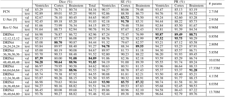
Results:We use the FCN, the U-Net, and the Res-U-Net as baselines. The baseline networks are compared to the DRINet with various growth rates. The results are displayed in Table II.

The FCN and the U-Net perform similarly well in terms of Dice. The results suggest that segmenting the CSF in ventricles is relatively easy while segmenting CSF around brainstem is challenging. As depicted in Fig. 6, the CSF around brainstem is likely to be misclassified. In addition, the skip connections in the U-Net do not improve the segmentation results in this case.

Changing the U-Net architecture into the Res-U-Net archi-tecture makes the network deeper and reduces the number of training parameters. According to [11], this change should only marginally influence on the results. However, the Dice score of the CSF around brainstem decreases under the Res-U-Net architecture. This result indicates that reducing param-eters is problematic although the network uses the residual connections.

The growth rate is the key hyper-parameter in the DRINet because it controls the network parameter space and per-formance. Changing the growth rate allows to compare the performance between baseline networks and the DRINets with a similar number of parameters. Table II shows the results evaluating the effects of growth rate. The DRINet with a growth rate of 12 has a similar number of parameters as the Res-U-Net. This DRINet segments the CSF around brainstem significantly better than the Res-U-Net. The DRINet with a

TABLE II

PERFORMANCE COMPARISON AMONG THE BASELINECNNS AND THEDRINET WITH DIFFERENT GROWTH RATES. THE NUMBERS UNDER THEDRINET INDICATE THE GROWTH RATES IN EACH DENSE CONNECTION BLOCK.

Dice (%) SE (%) PR (%) _{# params}

Ventricles Cortex Brainstem Total Ventricles Cortex Brainstem Ventricles Cortex Brainstem

FCN val 83.29 76.71 80.74 84.16 90.17 80.06 79.48 93.47 85.13 83.19 2.71M test 92.89 89.01 85.25 90.91 92.86 88.50 86.73 94.76 91.18 84.52 U-Net [5] val 82.67 76.10 80.45 84.65 90.07 83.72 78.50 93.24 82.60 83.28 2.91M test 92.45 89.18 85.20 91.03 92.18 91.70 85.31 94.44 88.22 85.73 Res-U-Net val 81.66 73.99 76.34 84.15 89.72 79.48 75.84 92.84 85.50 81.67 0.96M test 91.64 88.73 82.94 90.76 91.54 87.67 82.43 93.81 91.39 84.34 DRINet val 84.98 76.87 86.72 82.96 87.24 75.47 76.99 95.87 89.49 88.71 0.85M 12,12,12,12 test 92.13 87.77 86.08 89.37 88.76 82.78 82.99 97.52 95.75 90.29 DRINet val 85.08 80.70 90.87 84.44 91.32 79.67 82.57 93.21 87.12 85.58 _2.80M 24,24,24,24 test 93.84 89.97 88.40 91.27 94.78 88.34 89.55 94.27 93.23 87.91 DRINet val 85.00 80.19 90.08 84.67 89.97 81.73 81.18 94.30 85.57 86.71 5.85M 36,36,36,36 test 93.70 90.33 88.48 91.52 92.80 90.23 88.22 96.20 91.93 89.45 DRINet val 87.39 80.00 91.08 84.89 91.06 82.36 82.18 93.59 85.29 86.74 _10.03M 48,48,48,48 test 94.28 90.64 88.96 91.85 94.19 91.00 89.39 95.55 91.74 89.24 DRINet val 86.97 79.95 90.58 84.62 90.63 80.51 81.15 93.96 86.64 88.33 17.33M 64,64,64,64 test 94.15 90.20 88.96 91.53 94.27 88.78 87.43 95.37 93.37 91.28 DRINet val 85.74 79.38 87.92 84.55 90.88 81.81 82.21 93.50 85.40 85.21 _4.11M 12,24,36,48 test 93.87 90.26 88.15 91.50 93.95 90.32 88.91 95.38 91.77 88.15 DRINet val 86.98 79.63 90.84 84.69 93.90 85.75 87.32 90.74 81.58 81.30 8.03M 24,36,48,64 test 94.27 90.16 88.82 91.51 94.19 89.53 87.83 95.68 92.45 90.53 DRINet val 86.45 80.08 89.68 84.72 89.86 80.96 82.10 94.58 86.43 87.22 _13.70M 36,48,64,80 test 93.76 90.27 88.82 91.46 92.44 89.38 88.59 96.64 92.79 89.76

growth rate 24 is comparable to the FCN and the U-Net in terms of the size of parameter space. It performs better than the FCN and the U-Net in terms of the CSF in ventricles and around brainstem. If the growth rate increases to 48, the DRINet performs best in all three parts of the CSF segmentation, as well as the whole CSF segmentation. When the growth rate becomes very large (e.g. 64), the DRINet is likely to overfit and the performance decreases. In the following experiments, a growth rate of 48 is used.

Huang et al. [8] noted that a larger growth rate in the higher layers is beneficial for the performance of network. In our experiments, we evaluate this strategy using growth rates like 12, 24, 36, 48 in each dense connection block. Comparing DRINets using identical growth rate and increasing growth rates, which have similar number of parameters, the DRINets using increasing growth rates do not perform significantly better in any part of CSF segmentations.

Run time: Pre-processing was performed on a desktop PC with an Core i7-3770 processor and 32GB RAM. CNNs were trained and tested on an NVIDIA TITAN XP GPU processor except for the DRINets with large growth rates (e.g. 48, 64), which were trained on two GPUs to keep the batch size sufficiently large. On average it took 44.46s for the DRINet to segment the CSF in one image. The training time of the DRINet with the best performance was 21.37 hours. In contrast, the U-Net is faster with 11.44 hours for training and 23.56s per image for testing. Although the DRINet is slower, its run time is acceptable.

B. Multi-organ segmentation

Overview: Segmenting abdominal organs is important for clinical diagnosis and surgery planning [33]. There are two

major challenges in the multi-organ segmentation problem: 1) Abdominal organs are highly deformable and mobile and therefore can have various shapes and sizes; 2) the contrast between organs is often poor making it difficult to identify boundaries between organs.

Abdominal organ segmentation is a popular topic for which many solutions have been proposed. Many methods were based on statistical shape models [34] or multi-atlas segmen-tation [34]–[38]. Using recent deep learning approaches, the segmentation accuracy has significantly improved, particularly for smaller organs (e.g. pancreas). Furthermore, deep learning approaches are much faster than conventional methods [4], [39], [40].

Dataset:3D abdominal CT scans were used in this exper-iment to evaluate the performance of the DRINet. Image ac-quisition parameters and patient demographics for the dataset used here can be found in [37].

Pre-processing and augmentation were carried out in similar manner to those for CSF segmentation. The only difference is that in the CSF segmentation, the image intensity normaliza-tion is performed per slice while in this multi-organ segmen-tation task, the image intensity is normalized per volume. The

128×128 image patches were randomly cropped to develop the training set.

We used the same the experimental settings and CNN con-figurations as in the previous experiments, so no parameters tuning is performed in this experiment. The purpose is to validate the flexibility of the DRINet. Therefore, we only split the whole dataset into a training set (75 subjects) and a separate testing set (75 subjects).

Baseline: Again, the U-Net and the Res-U-Net are used as baselines. Table III displays the segmentation results. The

Fig. 6. The visual examples of multi-class CSF segmentations. The first column displays the original images. The second column shows the manual references. The following columns demonstrate the segmentations of the U-Net, the Res-U-Net, and the DRINet.

performance of the U-Net and the Res-U-Net is comparable. The Res-Net provides better PR but worse SE than the U-Net in segmenting the pancreas and kidneys. As mentioned above, the pancreas is the most challenging organ to segment because of its thin and various structure. The strength of the proposed DRINet is demonstrated by the fact that it is able to segment the challenging organs significantly better than the baseline CNNs approaches.

Comparison with existing methods: We compare the DRINet with existing methods evaluated on the same dataset. [36] and [37] proposed methods based on conventional ma-chine learning approaches. According to the results (displayed in Table IV) they have achieved fairly good segmentations in terms of kidneys, liver, and spleen. The method proposed by Tong et al. [37] is much faster than the one proposed by Wolz et al. [36]. The 3D FCN proposed by Roth et al. [4] is the state-of-the-art method based on deep CNNs. It is clear that the 3D FCN achieves significantly better results in the pancreas segmentation. Furthermore the inference time is significantly reduced. However, in terms of the other organs, namely the kidneys, liver, and spleen, the 3D FCN did not offer significant improvements.

The DRINet outperforms the 3D FCN achieving the

state-of-the-art based on this dataset. Specifically, it improves the pancreas segmentation further from the 3D FCN. In addition, the DRINet promotes the segmentation on other organs as well. Note that the DRINet is only based on 2D image slices without using 3D contextual information. Therefore, this experiments verifies the DRINet is powerful and robust in the multi-organ segmentation problem.

C. Brain Tumour Segmentation

Overview: Brain tumours are routinely diagnosed using multi-modal MRI, including native T1-weighted (T1), post-contrast T1-weighted (T1-Gd), T2-weighted (T2), and T2 fluid attenuated inversion recovery (FLAIR) image sequences [41]. Quantification of the tumours based on the multi-modal MRI benefits the diagnosis and treatment [42]. Segmenting tumours into necrotic and non-enhancing tumours, the peritumoral edema, and gadolinium enhancing tumours has been a popular research topic [43].

Dataset: We propose to use the training dataset of the BraTS 2017 challenge. There are 285 subjects in total and we randomly select 50 for training and the remaining 235 ones for testing. The segmentation is based on 2D patches of size of64×64. Since the training patch size is smaller compared to

TABLE III

PERFORMANCE COMPARISON AMONG THEU-NET,THERES-U-NET AND THEDRINET. THEDRINET OUTPERFORMED THE BASELINECNNS, PARTICULARLY IN TERMS OF THE PANCREAS.

Dice (%) SE (%) PR (%)

Pancreas Kidneys Liver Spleen Pancreas Kidneys Liver Spleen Pancreas Kidneys Liver Spleen

U-Net [5] 80.09 95.80 94.70 94.72 74.89 95.86 92.79 93.13 87.98 95.85 96.65 95.98

Res-U-Net 79.09 95.41 96.20 94.71 72.41 93.72 96.15 92.92 89.49 97.28 96.26 95.94

DRINet 83.42 95.96 96.57 95.64 80.29 95.84 96.69 95.63 87.95 96.20 96.47 96.13

Fig. 7. The visual examples of abdominal multi-organ segmentations. The first column displays the original images. The second column shows the manual references. The following columns demonstrate the segmentations of the U-Net, the Res-U-Net, and the DRINet.

TABLE IV

PERFORMANCE COMPARISON AMONG DIFFERENT ALGORITHMS. IT IS CLEAR THAT THEDRINET IS SUPERIOR TO THE EXISTING METHODS.

Dice (%) _{Time (h)}

Pancreas Kidneys Liver Spleen Wolz et al. [36] 69.60 92.50 94.00 92.00 51 Tong et al. [37] 69.80 93.40 94.90 91.90 0.5 Roth et al. [4] 82.20 - 95.40 92.80 0.07

DRINet 83.42 95.96 96.57 95.64 0.02

that in the previous experiments, all CNNs in this experiments have two downsampling and upsampling process and all the other network configurations are fixed. According to [43], the images have been preprocessed: images were co-registered into the same anatomical template; skulls were stripped; voxels were resampled to isotropic resolution (1mm3). We normalise the image intensities into zero mean and unit deviation. No post-processing trick is used in any case. The evaluation is based on the whole tumour region, the tumour core region, and the enhancing tumour core region, instead of individual

tumour structures.

Results: On this benchmark dataset, we evaluate the three key components of the DRINet: the dense connection block, the residual Inception block, and the unpooling block. We set the FCN as the baseline CNN and separately add one of the proposed blocks to verify its contribution. We also compare their performance with the U-Net and the DRINet.

Table V shows the results: In terms of the whole tumour structure, the added blocks do not affect the Dice scores signif-icantly. The dense connection block and the residual Inception block increase the sensitivity and the Hausdorff distances and decrease the specificity, which means they increase the number of false positives (FPs). In contrast, the unpooling block decreases the sensitivity and Hausdorff distance and increases the specificity, which means it reduces FPs but introduces FNs. Combining them together results in a trade-off between FNs and FPs. Therefore, the overall performance increases.

In terms of the tumour core and enhanced core, the three blocks increase the Dice scores and specificity while decreas-ing their sensitivity and Hausdorff distances. This means the overall performance for the segmentation of the tumour core

and the enhanced core is improved. However, since their sizes are fairly small, some FNs occur.

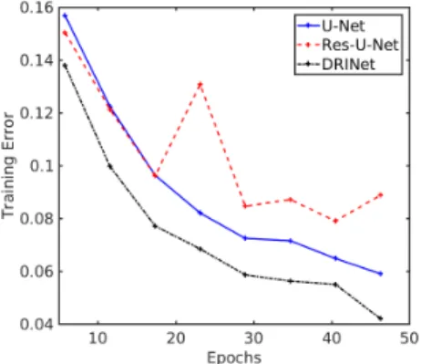
The DRINet with three powerful blocks achieves better segmentation results than the U-Net in terms of the dice scores, the sensitivity, and the Hausdorff distances. Regarding the Res-U-Net, since the parameter space is small, it cannot perform as well as the U-Net in this case. Fig. 8 shows that the training error of the Res-U-Net is larger than that of the U-Net and the DRINet. Therefore, the Dice coefficients given by the Res-U-Net on tumours are the worst among all the CNNs. According to the low sensitivity, the high specificity, and the low Hausdorff distance, it is clear that the segmentation results by the Res-U-Net have many FNs but few FPs.

Fig. 8. The training error comparisons among different CNNs.

V. DISCUSSION ANDCONCLUSION

In this paper, a novel CNN architecture, DRINet, is pro-posed. The DRINet has three key features, namely the use of dense connection blocks, residual inception blocks, and the unpooling blocks. These blocks deepen and widen the network significantly and the parameter space can be controlled via the growth rate. The gradient propagation is improved due to the dense connections and residual connections. As a result, the performance of the DRINet is significantly im-proved when compared to the standard U-Net. In addition, the DRINet architecture is highly flexible: Within a block, the convolution/deconvolution layers can be changed adaptively. It is therefore easy to integrate the blocks into other CNN architectures.

In this paper, we focus on evaluating the performance of the proposed DRINet and each of its components. The segmentation results of each problem can be improved using some domain knowledge and post-processing. For instance, in the brain CSF segmentation problem, a brain mask could be added. In the abdominal organ segmentation task, 3D contex-tual information could be included. In the BraTS problem, the CRF model could be used to remove FPs.

Among the three experiments, the multi-class CSF segmen-tation on CT images is novel. To the best of our knowledge, we are the first to attempt on this problem and the proposed DRINet results in good segmentation. In the future, we plan extend the proposed approach to segment lesions as well as CSF using a single DRINet. This is useful in clinical settings

for prognostication after stroke [44] or estimating cerebral haemorrhage risk [45], [46].

In the context of abdominal multi-organ segmentation, the DRINet achieves very good results although the segmentation is based on 2D CT image slices. Our results show that the DRINet improves the segmentation on small and various organs like pancreas as well as big organs like liver. It is of interest to extend its ability to segment more challenging organs such as arteries and veins, which could make the DRINet more useful in clinics.

A limitation of the DRINet approach is that the increase of the growth rate results in many more parameters, which may lead the training more difficult and testing slower. In the future, the research could focus on simplifying the network structure while maintaining its ability.

ACKNOWLEDGMENT

This work is supported by the NIHR Grant i4i: Decision-assist software for management of acute ischemic stroke using brain-imaging machine-learning (Ref: II-LA-0814-20007) and JSPS Kakenhi (26108006, 17K20099). We acknowledge the kind donation of the GPUs from the NVidia.

REFERENCES

[1] H. Greenspan, B. van Ginneken, and R. M. Summers, “Guest editorial deep learning in medical imaging: Overview and future promise of an exciting new technique,” IEEE Transactions on Medical Imaging, vol. 35, no. 5, pp. 1153–1159, 2016.

[2] A. de Brebisson and G. Montana, “Deep neural networks for anatomical brain segmentation,” inCVPR Workshops, 2015, pp. 20–28.

[3] M. Avendi, A. Kheradvar, and H. Jafarkhani, “A combined deep-learning and deformable-model approach to fully automatic segmentation of the left ventricle in cardiac MRI,” Medical Image Analysis, vol. 30, pp. 108–119, 2016.

[4] H. R. Roth, H. Oda, Y. Hayashi, M. Oda, N. Shimizu, M. Fujiwara, K. Misawa, and K. Mori, “Hierarchical 3D fully convolutional networks for multi-organ segmentation,”arXiv preprint:1704.06382, 2017. [5] O. Ronneberger, P. Fischer, and T. Brox, “U-net: Convolutional networks

for biomedical image segmentation,” inMICCAI, 2015, pp. 234–241. [6] ¨O. C¸ ic¸ek, A. Abdulkadir, S. S. Lienkamp, T. Brox, and O. Ronneberger,

“3D U-net: learning dense volumetric segmentation from sparse anno-tation,” inMICCAI, 2016, pp. 424–432.

[7] G. Huang, Z. Liu, K. Q. Weinberger, and L. van der Maaten, “Densely connected convolutional networks,” inCVPR, 2016, pp. 4700–4708. [8] G. Huang, D. Chen, T. Li, F. Wu, L. van der Maaten, and K. Q.

Weinberger, “Multi-scale dense convolutional networks for efficient prediction,” inICLR, 2018.

[9] C. Szegedy, S. Ioffe, V. Vanhoucke, and A. A. Alemi, “Inception-v4, Inception-ResNet and the impact of residual connections on learning,” inAAAI, 2017, pp. 4278–4284.

[10] C. Szegedy, W. Liu, Y. Jia, P. Sermanet, S. Reed, D. Anguelov, D. Erhan, V. Vanhoucke, and A. Rabinovich, “Going deeper with convolutions,” inCVPR, 2015, pp. 1–9.

[11] K. He, X. Zhang, S. Ren, and J. Sun, “Deep residual learning for image recognition,” inCVPR, 2016, pp. 770–778.

[12] L.-C. Chen, G. Papandreou, I. Kokkinos, K. Murphy, and A. L. Yuille, “DeepLab: semantic image segmentation with deep convolutional nets, atrous convolution, and fully connected CRFs,” IEEE Transactions on Pattern Analysis and Machine Intelligence, vol. PP, no. 99, pp. 1–1, 2017.

[13] L.-C. Chen, G. Papandreou, F. Schroff, and H. Adam, “Rethinking atrous convolution for semantic image segmentation,” arXiv preprint arXiv:1706.05587, 2017.

[14] S. J´egou, M. Drozdzal, D. Vazquez, A. Romero, and Y. Bengio, “The one hundred layers tiramisu: Fully convolutional densenets for semantic segmentation,” inCVPR Workshops, 2017, pp. 1175–1183.

[15] H. Zhao, J. Shi, X. Qi, X. Wang, and J. Jia, “Pyramid scene parsing network,” inCVPR, 2017, pp. 2881–2890.

TABLE V

THE SEGMENTATION RESULTS OF DIFFERENT NETWORKS. THE ENTRIES IN BOLD HIGHLIGHT THE BEST COMPARABLE RESULTS.

Network _Whole Dice (%)_{Core Enh. Whole} SE (%)_{Core Enh. Whole} SP (%)_{Core Enh. Whole}Hausdorff95 (mm)_{Core Enh.} U-Net [5] 81.51 71.30 63.05 81.69 72.51 79.70 99.86 99.92 99.94 42.07 34.44 36.46 Res-U-Net 71.50 67.75 60.06 60.25 66.06 68.27 99.97 99.93 99.97 21.98 25.00 27.56 FCN 81.42 70.4 61.49 80.84 77.12 80.76 99.85 99.80 99.92 42.19 47.24 44.08 FCN+dense 81.09 71.98 63.29 84.90 74.81 78.56 99.80 99.91 99.95 48.34 39.36 36.56 FCN+RI 81.89 72.30 63.25 85.26 74.29 78.02 99.82 99.91 99.95 47.38 36.49 33.97 FCN+unpool 81.81 71.43 63.93 78.56 70.53 75.80 99.91 99.94 99.96 33.37 28.39 27.12 DRINet 83.47 73.21 64.98 84.53 74.93 80.35 99.86 99.92 99.94 36.4 25.59 30.31

[16] S. Ioffe and C. Szegedy, “Batch normalization: Accelerating deep network training by reducing internal covariate shift,” inICML, 2015, pp. 448–456.

[17] L. Chen, P. Bentley, and D. Rueckert, “Fully automatic acute ischemic lesion segmentation in DWI using convolutional neural networks,”

NeuroImage: Clinical, 2017.

[18] D. Kingma and J. Ba, “Adam: A method for stochastic optimization,” inICLR, 2015.

[19] N. Sanossian, K. A. Fu, D. S. Liebeskind, S. Starkman, S. Hamilton, J. P. Villablanca, A. M. Burgos, R. Conwit, and J. L. Saver, “Utilization of emergent neuroimaging for thrombolysis-eligible stroke patients,”

Journal of Neuroimaging, vol. 27, no. 1, pp. 59–64, 2017.

[20] I. K. Pople, “Hydrocephalus and shunts: what the neurologist should know,”Journal of Neurology, Neurosurgery & Psychiatry, vol. 73, no. suppl 1, pp. i17–i22, 2002.

[21] M. A. Williams and N. R. Relkin, “Diagnosis and management of id-iopathic normal-pressure hydrocephalus,”Neurology: Clinical Practice, vol. 3, no. 5, pp. 375–385, 2013.

[22] A. V. Kulkarni, J. M. Drake, D. C. Armstrong, and P. B. Dirks, “Measurement of ventricular size: reliability of the frontal and occipital horn ratio compared to subjective assessment,”Pediatric Neurosurgery, vol. 31, no. 2, pp. 65–70, 1999.

[23] F. Pasquier, D. Leys, J. G. Weerts, F. Mounier-Vehier, F. Barkhof, and P. Scheltens, “Inter-and intraobserver reproducibility of cerebral atrophy assessment on MRI scans with hemispheric infarcts,”European Neurology, vol. 36, no. 5, pp. 268–272, 1996.

[24] T. Sandor, D. Metcalf, and Y.-J. Kim, “Segmentation of brain CT images using the concept of region growing,” International Journal of Bio-Medical Computing, vol. 29, no. 2, pp. 133–147, 1991.

[25] U. E. Ruttimann, E. M. Joyce, D. E. Rio, and M. J. Eckardt, “Fully au-tomated segmentation of cerebrospinal fluid in computed tomography,”

Psychiatry Research: Neuroimaging, vol. 50, no. 2, pp. 101–119, 1993. [26] T. H. Lee, M. F. A. Fauzi, and R. Komiya, “Segmentation of CT brain images using K-means and EM clustering,” inFifth International Conference on Computer Graphics, Imaging and Visualisation, 2008, pp. 339–344.

[27] ——, “Segmentation of CT brain images using unsupervised cluster-ings,”Journal of Visualization, vol. 12, no. 2, pp. 131–138, 2009. [28] W. Chen and K. Najarian, “Segmentation of ventricles in brain CT

im-ages using gaussian mixture model method,” inInternational Conference on Complex Medical Engineering, 2009, pp. 1–6.

[29] V. Gupta, W. Ambrosius, G. Qian, A. Blazejewska, R. Kazmierski, A. Urbanik, and W. L. Nowinski, “Automatic segmentation of cere-brospinal fluid, white and gray matter in unenhanced computed tomog-raphy images,”Academic Radiology, vol. 17, no. 11, pp. 1350–1358, 2010.

[30] L. Poh, V. Gupta, A. Johnson, R. Kazmierski, and W. L. Nowinski, “Au-tomatic segmentation of ventricular cerebrospinal fluid from ischemic stroke CT images,”Neuroinformatics, vol. 10, no. 2, pp. 159–172, 2012. [31] X. Qian, J. Wang, S. Guo, and Q. Li, “An active contour model for medical image segmentation with application to brain CT image,”

Medical Physics, vol. 40, no. 2, 2013.

[32] X. Qian, Y. Lin, Y. Zhao, X. Yue, B. Lu, and J. Wang, “Objective ventricle segmentation in brain CT with ischemic stroke based on anatomical knowledge,” BioMed Research International, vol. 2017, 2017.

[33] M. G. Linguraru, J. A. Pura, V. Pamulapati, and R. M. Summers, “Statistical 4D graphs for multi-organ abdominal segmentation from multiphase CT,”Medical Image Analysis, vol. 16, no. 4, pp. 904–914, 2012.

[34] T. Okada, R. Shimada, M. Hori, M. Nakamoto, Y.-W. Chen, H. Naka-mura, and Y. Sato, “Automated segmentation of the liver from 3D CT images using probabilistic atlas and multilevel statistical shape model,”

Academic Radiology, vol. 15, no. 11, pp. 1390–1403, 2008.

[35] Z. Wang, K. K. Bhatia, B. Glocker, A. Marvao, T. Dawes, K. Misawa, K. Mori, and D. Rueckert, “Geodesic patch-based segmentation,” in

MICCAI, 2014, pp. 666–673.

[36] R. Wolz, C. Chu, K. Misawa, M. Fujiwara, K. Mori, and D. Rueckert, “Automated abdominal multi-organ segmentation with subject-specific atlas generation,”IEEE Transactions on Medical Imaging, vol. 32, no. 9, pp. 1723–1730, 2013.

[37] T. Tong, R. Wolz, Z. Wang, Q. Gao, K. Misawa, M. Fujiwara, K. Mori, J. V. Hajnal, and D. Rueckert, “Discriminative dictionary learning for abdominal multi-organ segmentation,”Medical Image Analysis, vol. 23, no. 1, pp. 92–104, 2015.

[38] C. Chu, M. Oda, T. Kitasaka, K. Misawa, M. Fujiwara, Y. Hayashi, Y. Nimura, D. Rueckert, and K. Mori, “Multi-organ segmentation based on spatially-divided probabilistic atlas from 3D abdominal CT images,” inMICCAI, 2013, pp. 165–172.

[39] H. R. Roth, L. Lu, N. Lay, A. P. Harrison, A. Farag, A. Sohn, and R. M. Summers, “Spatial aggregation of holistically-nested convolutional neu-ral networks for automated pancreas localization and segmentation,”

arXiv preprint:1702.00045, 2017.

[40] J. Cai, L. Lu, Y. Xie, F. Xing, and L. Yang, “Improving deep pancreas segmentation in CT and MRI images via recurrent neural contextual learning and direct loss function,”arXiv preprint:1707.04912, 2017. [41] S. Bakas, H. Akbari, A. Sotiras, M. Bilello, M. Rozycki, J. S. Kirby,

J. B. Freymann, K. Farahani, and C. Davatzikos, “Advancing the cancer genome atlas glioma mri collections with expert segmentation labels and radiomic features,”Scientific data, vol. 4, p. 170117, 2017.

[42] S. Bakas, H. Akbari, A. Sotiras, M. Bilello, M. Rozycki, J. Kirby, J. Freymann, K. Farahani, and C. Davatzikos, “Segmentation labels and radiomic features for the pre-operative scans of the tcga-lgg collection,”

The Cancer Imaging Archive, 2017.

[43] B. H. Menze, A. Jakab, S. Bauer, J. Kalpathy-Cramer, K. Farahani, J. Kirby, Y. Burren, N. Porz, J. Slotboom, R. Wiest et al., “The multimodal brain tumor image segmentation benchmark (brats),”IEEE Transactions on Medical Imaging, vol. 34, no. 10, pp. 1993–2024, 2015. [44] I.-. C. Groupet al., “Association between brain imaging signs, early and late outcomes, and response to intravenous alteplase after acute is-chaemic stroke in the third International Stroke Trial (IST-3): secondary analysis of a randomised controlled trial,”The Lancet Neurology, vol. 14, no. 5, pp. 485–496, 2015.

[45] P. Fotiadis, S. van Rooden, J. van der Grond, A. Schultz, S. Martinez-Ramirez, E. Auriel, Y. Reijmer, A. M. van Opstal, A. Ayres, K. M. Schwab et al., “Cortical atrophy in patients with cerebral amyloid angiopathy: a case-control study,”The Lancet Neurology, vol. 15, no. 8, pp. 811–819, 2016.

[46] C. M. Dunham, D. A. Hoffman, G. S. Huang, L. A. Omert, D. J. Gemmel, and R. Merrell, “Traumatic intracranial hemorrhage correlates with preinjury brain atrophy, but not with antithrombotic agent use: a retrospective study,”PloS One, vol. 9, no. 10, p. e109473, 2014.