Boston University
OpenBU
http://open.bu.edu
BU Open Access Articles BU Open Access Articles
2019-02-01
Reinforcement learning for UAV
attitude control
This work was made openly accessible by BU Faculty. Please
share
how this access benefits you.
Your story matters.
Version
Citation (published version): William Koch, Renato Mancuso, Richard West, Azer Bestavros. 2019.
"Reinforcement Learning for UAV Attitude Control." ACM Transactions
on Cyber-Physical Systems, Volume 2, Issue Feb 2019, pp. 1 - 21.
https://doi.org/10.1145/3301273
https://hdl.handle.net/2144/40560
Boston University
Reinforcement Learning for UAV Attitude Control
William Koch, Renato Mancuso, Richard West, Azer Bestavros
Boston University Boston, MA 02215
{wfkoch, rmancuso, richwest, best}@bu.edu
Abstract—Autopilot systems are typically composed of an “inner loop” providing stability and control, while an “outer loop” is responsible for mission-level objectives, e.g. way-point navigation. Autopilot systems for UAVs are predominately im-plemented using Proportional, Integral Derivative (PID) control systems, which have demonstrated exceptional performance in stable environments. However more sophisticated control is required to operate in unpredictable, and harsh environments. Intelligent flight control systems is an active area of research addressing limitations of PID control most recently through the use of reinforcement learning (RL) which has had success in other applications such as robotics. However previous work has focused primarily on using RL at the mission-level controller. In this work, we investigate the performance and accuracy of the inner control loop providing attitude control when using intelligent flight control systems trained with the state-of-the-art RL algorithms, Deep Deterministic Gradient Policy (DDGP), Trust Region Policy Optimization (TRPO) and Proximal Policy Optimization (PPO). To investigate these unknowns we first developed an open-source high-fidelity simulation environment to train a flight controller attitude control of a quadrotor through RL. We then use our environment to compare their performance to that of a PID controller to identify if using RL is appropriate in high-precision, time-critical flight control.
I. INTRODUCTION
Over the last decade there has been an uptrend in the popularity of Unmanned Aerial Vehicles (UAVs). In particular, quadrotors have received significant attention in the research community where a significant number of seminal results and applications has been proposed and experimented. This recent growth is primarily attributed to the drop in cost of onboard sensors, actuators and small-scale embedded computing plat-forms. Despite the significant progress, flight control is still considered an open research topic. On the one hand, flight control inherently implies the ability to perform highly time-sensitive sensory data acquisition, processing and computation of forces to apply to the aircraft actuators. On the other hand, it is desirable that UAV flight controllers are able to tolerate faults; adapt to changes in the payload and/or the environment; and to optimize flight trajectory, to name a few.
Autopilot systems for UAVs are typically composed of an “inner loop” responsible for aircraft stabilization and control, and an “outer loop” to provide mission level objectives (e.g.
way-point navigation). Flight control systems for UAVs are predominately implemented using the Proportional, Integral Derivative (PID) control systems. PIDs have demonstrated exceptional performance in many circumstances, including in the context of drone racing, where precision and agility are
key. In stable environments a PID controller exhibits close-to-ideal performance. When exposed to unknown dynamics (e.g.
wind, variable payloads, voltage sag, etc), however, a PID controller can be far from optimal [1]. For next-generation flight control systems to be intelligent, a way needs to be devised to incorporate adaptability to mutable dynamics and environment.
The development of intelligent flight control systems is an active area of research [2], specifically through the use of artificial neural networks which are an attractive option given they are universal approximators and resistant to noise [3].
Online learning methods (e.g. [4]) have the advantage of learning the aircraft dynamics in real-time. The main limitation with online learning is that the flight control system is only knowledgeable of its past experiences. It follows that its performances are limited when exposed to a new event. Train-ing models offline usTrain-ingsupervised learning is problematic as data is expensive to obtain and derived from inaccurate representations of the underlying aircraft dynamics (e.g.flight data from a similar aircraft using PID control) which can lead to suboptimal control policies [5], [6], [7]. To construct high-performance intelligent flight control systems it is necessary to use a hybrid approach. First, accurate offline models are used to construct a baseline controller, while online learning provides fine tuning and real-time adaptation.
An alternative to supervised learning for creating offline models is known as reinforcement learning (RL). In RL an agent is given a reward for every action it makes in an environment with the objective to maximize the rewards over time. Using RL it is possible to develop optimal control policies for a UAV without making any assumptions about the aircraft dynamics. Recent work has shown RL to be effective for UAV autopilots, providing adequate path tracking [8]. Nonetheless, previous work on intelligent flight control sys-tems has primarily focused on guidance and navigation. It remains unclear what level of control accuracy can be achieved when using intelligent control for time-sensitive attitude con-trol —i.e.the “inner loop”. Determining the achievable level of accuracy is critical in establishing for what applications intelligent flight control is indeed suitable. For instance, high precision and accuracy is necessary for proximity or indoor flight. But accuracy may be sacrificed in larger outdoor spaces where adaptability is of the utmost importance due to the unpredictability of the environment.
In this paper we study the accuracy and precision of attitude control provided by intelligent flight controllers trained using
RL. While we specifically focus on the creation of controllers for the Iris quadcopter [9], the methods developed hereby apply to a wide range of multi-rotor UAVs, and can also be extended to fixed-wing aircraft. We develop a novel training environment called GYMFC with the use of a high fidelity physics simulator for the agent to learn attitude control. GYM FC is an OpenAI Environment [10] providing a common interface for researchers to develop intelligent flight control systems. The simulated environment consists of an Iris quad-copter digital replica ordigital twin[11] with the intention of eventually be used to transfer the trained controller to physical hardware. Controllers are trained using state-of-the-art RL al-gorithms: Deep Deterministic Gradient Policy (DDGP), Trust Region Policy Optimization (TRPO), and Proximal Policy Optimization (PPO). We then compare the performance of our synthesized controllers with that of a PID controller. Our evaluation finds that controllers trained using PPO outperform PID control and are capable of exceptional performance. To summarize, this paper makes the following contributions:
• GYM FC, an open source [12] environment for devel-oping intelligent attitude flight controller providing the research community a tool to progress performance.
• A learning architecture for attitude control utilizing digi-tal twinning concepts for minimal effort when transferring trained controllers into hardware.
• An evaluation for state-of-the-art RL algorithms, such as Deep Deterministic Gradient Policy (DDGP), Trust Region Policy Optimization (TRPO), and Proximal Policy Optimization (PPO), learning policies for aircraft attitude control. As a first work in this direction, our evaluation also establishes a baseline for future work.
• An analysis of intelligent flight control performance de-veloped with RL compared to traditional PID control. The remainder of this paper is organized as follows. In Section II we provide an overview of the quadcopter flight dynamics and reinforcement learning. Next, in Section III we briefly survey existing literature on intelligent flight control. In Section IV we present our training environment and use this environment to evaluate RL performance for flight control in Section V. Finally Section VI concludes the paper and provides a number of future research directions.
II. BACKGROUND
In this section we provide a brief overview of quadcopter flight dynamics required to understand this work, and an introduction to developing flight control systems with rein-forcement learning.
A. Quadcopter Flight Dynamics
A quadcopter is an aircraft with six degrees of freedom (DOF), three rotational and three translational. With four control inputs (one to each motor) this results in an under-actuated system that requires an onboard computer to compute motor signals to provide stable flight. We indicate withωi, i∈
1, . . . , M the rotation speed of each rotor whereM = 4is the total number of motors for a quadcopter. These have a direct
Z X Y ψ θ φ
(a) Axis of rotation
4
3
4
3
2
1
(b) Roll right4
3
2
1
(c) Pitch forward2
4
4
3
4
3
2
1
(d) Yaw clockwiseimpact on the resulting Euler angles φ, θ, ψ, i.e. roll, pitch, yaw respectively which provide rotation inD= 3dimensions. Moreover, they produce a certain amount of upward thrust, indicated withf.
The aerodynamic effect that each ωi produces depends upon the configuration of the motors. The most popular configuration is an “X” configuration, depicted in Figure 1a which has the motors mounted in an “X” formation relative to what is considered the front of the aircraft. This configuration provides more stability compared to a “+” configuration which in contrast has its motor configuration rotated an additional
45◦ along the z-axis. This is due to the differences in torque
generated along each axis of rotation in respect to the distance of the motor from the axis. The aerodynamic affectuthat each rotor speed ωi has on thrust and Euler angles, is given by:
uf =b(ω12+ω 2 2+ω 2 3+ω 2 4) (1) uφ=b(ω12+ω 2 2−ω 2 3−ω 2 4) (2) uθ=b(ω12−ω22+ω23−ω42) (3) uψ=b(ω12−ω 2 2−ω 2 3+ω 2 4) (4)
whereuf, uφ, uθ, uψ is the thrust, roll, pitch, and yaw effect respectively, while b is a thrust factor that captures propeller geometry and frame characteristics. For further details about the mathematical models of quadcopter dynamics please refer to [13].
To perform a rotational movement the velocity of each rotor is manipulated according to the relationship expressed in Equation 4 and as illustrated in Figure 1b, 1c, 1d. For example, to roll right (Figure 1b) more thrust is delivered to motors 3 and 4. Yaw (Figure 1d) is not achieved directly through difference in thrust generated by the rotor as roll and pitch are, but instead through a difference in torque in the
rotation speed of rotors spinning in opposite directions. For example, as shown in Figure 1d, higher rotation speed for rotors 1 and 4 allow the aircraft to yaw clockwise. Because a net positive torque counter-clockwise causes the aircraft to rotate clockwise due to Newton’s second law of motion.
Attitude, in respect to orientation of a quadcopter, can be expressed by its angular velocities of each axis Ω = [Ωφ,Ωθ,Ωψ]. The objective of attitude control is to compute the required motor signals to achieve some desired attitude
Ω∗.
In autopilot systems attitude control is executed as an inner control loop and is time-sensitive. Once the desired attitude is achieved, translational movement (in the X, Y, Z direction) is accomplished by applying thrust proportional to each motor.
In commercial quadcopter, the vast if not all use PID attitude control. A PID controller is a linear feedback controller expressed mathematically as,
u(t) =Kpe(t) +Ki Z t 0 e(τ)dτ+Kd de(t) dt (5)
whereKp, Ki, Kd are configurable constant gains andu(t)is the control signal. The effect of each term can be thought of as the P term considers the current error, the I term considers the history of errors and the D term estimates the future error. For attitude control in a quadcopter aircraft there is PID control for each roll, pitch and yaw axis. At each cycle in the inner loop, each PID sum is computed for each axis and then these values are translated into the amount of power to deliver to each motor through a process called mixing. Mixing uses a table consisting of constants describing the geometry of the frame to determine how the axis control signals are summed based on the torques that will be generated by the length of each arm (recall differences between “X” and “+” frames). The control signal for each motor yi is loosely defined as,
yi=f m(i,φ)uφ+m(i,θ)uθ+m(i,ψ)uψ (6) where m(i,φ), m(i,θ), m(i,ψ) are the mixer values for motor i
andf is the throttle coefficient.
B. Reinforcement Learning
In this work we consider a neural network flight controller as an agent interacting with an Iris quadcopter [9] in a high fidelity physics simulated environment E, more specifically using the Gazebo simulator [14].
At each discrete time-step t, the agent receives an obser-vation xt from the environments consisting of the angular velocity error of each axise= Ω∗
−Ωand the angular velocity of each rotor ωi which are obtained from the quadcopter’s gyroscope and electronic speed controller (ESC) respectively. These observations are in the continuous observation spaces xt ∈ R(M+D). Once the observation is received, the agent executes an action at within E. In return the agent receives a single numerical reward rt indicating the performance of this action. The action is also in a continuous action space at ∈RM and corresponds to the four control signals sent to each motor. Because the agent is only receiving this sensor
data it is unaware of the physical environment and the aircraft dynamics and therefore E is only partially observed by the agent. Motivated by [15] we consider the state to be a sequence of the past observations and actionsst=xi, ai, . . . , at−1, xt. The interaction between the agent andE is formally defined as a Markov decision processes (MDP) where the state tran-sitions are defined as the probability of transitioning to state s0 given the current state and action are sandarespectively,
P r{st+1 = s0|st = s, at = a}. The behavior of the agent is defined by its policy π which is essentially a mapping of what action should be taken for a particular state. The objective of the agent is to maximize the returned reward overtime to develop an optimal policy. We welcome the reader to refer to [16] for further details on reinforcement learning.
Up until recently control in continuous action space was considered difficult for RL. Significant progress has been made combining the power of neural networks with RL. In this work we elected to use Deep Deterministic Gradient Policy (DDGP) [17] and Trust Region Policy Optimization (TRPO) [18] due to the recent use of these algorithms for quadcopter navigation control [8]. DDPG provides improvement to Deep Q-Network (DQN) [15] for the continuous action domain. It employs an actor-critic architecture using two neural networks for each actor and critic. It is also model-free algorithm meaning it can learn the policy without having to first generate a model. TRPO is similar to natural gradient policy methods however this method guarantees monotonic improvements. We additionally include a third algorithm for our analysis called Proximal Policy Optimization (PPO) [19]. PPO is known to out perform other state-of-the-art methods in challenging environments. PPO is also a policy gradient method and has similarities to TRPO while being easier to implement and tune.
III. RELATEDWORK
Aviation has a rich history in flight control dating back to the 1960s. During this time supersonic aircraft were being developed which demanded more sophisticated dynamic flight control than what a static linear controller could provide. Gain scheduling [20] was developed allowing multiple linear controllers of different configurations to be used in designated operating regions. This however was inflexible and insuffi-cient for handling the nonlinear dynamics at high speeds but paved way for adaptive control. For a period of time many experimental adaptive controllers were being tested but were unstable. Later advances were made to increase stability with model reference adaptive control (MRAC) [21], and L1 [22]
which provided reference models during adaptation. As the cost of small scale embedded computing platforms dropped, intelligent flight control options became realistic and have been actively researched over the last decade to design flight control solutions that are able toadapt, but also tolearn.
As performance demands for UAVs continues to increase we are beginning to see signs that flight control history repeats itself. The popular high performance drone racing firmware Betaflight [23] has recently added gain scheduler to adjust PID gains depending on throttle and voltage levels. Intelligent
PID flight control [24] methods have been proposed in which PID gains are dynamically updated online providing adaptive control as the environment changes. However these solutions still inherit disadvantages associated with PID control, such as integral windup, need for mixing, and most significantly, they are feedback controllers and therefore inherentlyreactive. On the other hand feedforward control (or predictive control) is
proactive, and allows the controller to output control signals before an error occur. For feedforward control, a model of the system must exist. Learning-based intelligent control has been proposed to develop models of the aircraft for predictive control using artificial neural networks.
Notable work by Dierks et. al. [4] proposes an intelligent flight control system constructed with neural networks to learn the quadcopter dynamics, online, to navigate along a specified path. This method allows the aircraft to adapt in real-time to external disturbances and unmodeled dynamics. Matlab simulations demonstrate that their approach outper-forms a PID controller in the presence of unknown dynamics, specifically in regards to control effort required to track the desired trajectory. Nonetheless the proposed approach does requires prior knowledge of the aircraft mass and moments of inertia to estimate velocities. Online learning is an essential component to constructing a complete intelligent flight control system. It is fundamental however to develop accurate offline models to account for uncertainties encountered during online learning [2]. To build offline models, previous work has used supervised learning to train intelligent flight control systems using a variety of data sources such as test trajectories [5], and PID step responses [6]. The limitation of this approach is that training data may not accurately reflect the underlying dynamics. In general, supervised learning on its own is not ideal for interactive problems such as control [16].
Reinforcement learning has similar goals to adaptive control in which a policy improves overtime interacting with its envi-ronment. The first use of reinforcement learning in quadcopter control was presented by Waslander et. al. [25] for altitude control. The authors developed a model-based reinforcement learning algorithm to search for an optimal control policy. The controller was rewarded for accurate tracking and damping. Their design provided significant improvements in stabiliza-tion in comparison to linear control system. More recently Hwangbo et. al. [8] has used reinforcement learning for quadcopter control, particularly for navigation control. They developed a novel deterministic on-policy learning algorithm that outperformed TRPO [18] and DDPG [17] in regards to training time. Furthermore the authors validated their results in the real world, transferring their simulated model to a physical quadcopter. Path tracking turned out to be adequate. Notably, the authors discovered major differences transferring from simulation to the real world. Known as the reality gap, transferring from simulation to the real-world has been researched extensively as being problematic without taking additional steps to increase realism in the simulator [26], [3]. The vast majority of prior work has focused on performance of navigation and guidance. There is limited and insufficient
data justifying the accuracy and precision of neural-network-based intelligent attitude flight control and none to our knowl-edge for controllers trained using RL. Furthermore this work uses physics simulations in contrast to mathematical models of the aircraft and environments used in aforementioned prior work for increased realism. The goal of this work is to provide a platform for training attitude controllers with RL, and to provide performance baselines in regards to attitude controller accuracy.
IV. ENVIRONMENT
In this section we describe our learning environment GYM FC for developing intelligent flight control systems using RL. The goal of proposed environment is to allow the agent to learn attitude control of an aircraft with only the knowledge of the number of actuators. GYMFC includes both anepisodic task and a continuous task. In an episodic task, the agent is required to learn a policy for responding to individual angular velocity commands. This allows the agents to learn the step response from rest for a given command, allowing its performance to be accurately measured. Episodic tasks however are not reflective of realistic flight conditions. For this reason, in a continuous task, pulses with random widths and amplitudes are continuously generated, and correspond to angular velocity set-points. The agent must respond accord-ingly and track the desired target over time. In Section V we evaluate our synthesized controllers via episodic tasks, but we have strong experimental evidence that training via episodic tasks produces controllers that behave correctly in continuous tasks as well (Appendix A).
GYM FC has a multi-layer hierarchical architecture com-posed of three layers: (i) a digital twin layer, (ii) a commu-nication layer, and (iii) an agent-environment interface layer. This design decision was made to clearly establish roles and allow layer implementations to change (e.g.to use a different simulator) without affecting other layers as long as the layer-to-layer interfaces remain intact. A high level overview of the environment architecture is illustrated in Figure 2. We will now discuss in greater detail each layer with a bottom-up approach.
A. Digital Twin Layer
At the heart of the learning environment is a high fidelity physics simulator which provides functionality and realism that is hard to achieve with an abstract mathematical model of the aircraft and environment. One of the primary design goals of GYMFC is to minimize the effort required to transfer a controller from the learning environment into the final platform. For this reason, the simulated environment exposes identical interfaces to actuators and sensors as they would exist in the physical world. In the ideal case the agent should not be able to distinguish between interaction with the simulated world (i.e.its digital twin) and its hardware counter part. In this work we use the Gazebo simulator [14] in light of its maturity, flexibility, extensive documentation, and active community.
Fig. 2: Overview of environment architecture, GYMFC. Blue blocks with dashed borders are implementations developed for this work.
In a nutshell, the digital twin layer is defined by (i) the simulated world, and (ii) its interfaces to the above commu-nication layer (see Figure 2).
Simulated World The simulated world is constructed
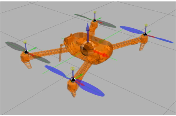
specifically for UAV attitude control in mind. The technique we developed allows attitude control to be accomplished independently of guidance and/or navigation control. This is achieved by fixing the center of mass of the aircraft to a ball joint in the world, allowing it to rotate freely in any direction, which would be impractical if not impossible to achieved in the real world due to gimbal lock and friction of such an apparatus. In this work the aircraft to be controlled in the environment is modeled off of the Iris quadcopter [9] with a weight of 1.5 Kg, and 550 mm motor-to-motor distance. An illustration of the quadcopter in the environment is displayed in Figure 3. Note during training Gazebo runs in headless mode without this user interface to increase simulation speed. This architecture however can be used with any multicopter as long as a digital twin can be constructed. Helicopters and multicopters represent excellent candidates for our setup because they can achieve a full range of rotations along all the three axes. This is typically not the case with fixed-wing aircraft. Our design can however be expanded to support fixed-wing by simulating airflow over the control surfaces for attitude control. Gazebo already integrates a set of tools to perform airflow simulation.
Interface The digital twin layer provides two command
interfaces to the communication layer: simulation reset and motor update. Simulation reset commands are supported by Gazebo’s API and are not part of our implementation. Motor updates are provided by a UDP server. We hereby discuss our approach to developing this interface.
In order to keep synchronicity between the simulated world and the controller of the digital twin, the pace at which
Fig. 3: The Iris quadcopter in Gazebo one meter above the ground. The body is transparent to show where the center of mass is linked as a ball joint to the world. Arrows represent the various joints used in the model.
simulation should progress is directly enforced. This is pos-sible by controlling the simulator step-by-step. In our initial approach, Gazebo’s Google Protobuf [27] API was used, with a specific message to progress by a single simulation step. By subscribing to status messages (which include the current simulation step) it is possible to determine when a step has completed and to ensure synchronization. However as we attempted to increase the rate of advertising step messages, we discovered that the rate of status messages is capped at 5 Hz. Such a limitation introduces a consistent bottleneck in the simulation/learning pipeline. Furthermore it was found that Gazebo silently drops messages it cannot process.
A set of important modifications were made to increase ex-periment throughput. The key idea was to allow motor update commands to directly drive the simulation clock. By default Gazebo comes pre-installed with an ArduPilot Arducopter [28] plugin to receive motor updates through a UDP server. These motor updates are in the form of a pulse width modulation (PWM) signals. At the same time, sensor readings from the inertial measurement unit (IMU) on board the aircraft is sent over a second UDP channel. Arducopter is an open source multicopter firmware and its plugin was developed to support software in the loop (SITL).
We derived our Aircraft Plugin from the Arducopter plugin with the following modifications (as well as those discussed in Section IV-B). Upon receiving a motor command, the motor forces are updated as normal but then a simulation step is executed. Sensor data is read and then sent back as a response to the client over the same UDP channel. In addition to the IMU sensor data we also simulate sensor data obtained from the electronic speed controller (ESC). The ESC provides the angular velocities of each rotor, which are relayed to the client
too.Implementing our Aircraft Plugin with this approach
successfully allowed us to work around the limitations of the Google Protobuf API and increased step throughput by over 200 times.
B. Communication Layer
The communication layer is positioned in between the digital twin and the agent-environment interface. This layer manages the low-level communication channel to the aircraft and simulation control. The primary function of this layer is to export a high-level synchronized API to the higher layers for interacting with the digital twin which uses asynchronous communication protocols. This layer provides the commands
pwm_write andreset to the agent-environment interface layer.
The function call pwm_write takes as input a vector of PWM values for each actuator, corresponding to the control inputu(t). These PWM values correspond to the same values that would be sent to an ESC on a physical UAV. The PWM values are translated to a normalized format expected by the Aircraft Plugin, and then packed into a UDP packet for trans-mission to the Aircraft Plugin UDP server. The communication layer blocks until a response is received from the Aircraft Plugin, forcing synchronized writes for the above layers. The UDP reply is unpacked and returned in response.
During the learning process the simulated environment must be reset at the beginning of each learning episode. Ideally one could use the gz command line utility included with the Gazebo installation which is lightweight and does not require additional dependencies. Unfortunately there is a known socket handle leak [29] that causes Gazebo to crash if the command is issued more than the maximum number of open files allowed by the operating system. Given we are running thousands episodes during training this was not an option for us. Instead we opted to use the Google Protobuffer interface so we did not have to deploy a patched version of the utility on our test servers. Because resets only occur at the beginning of a training session and are not in the critical processing loop using Google Protobuffers here is acceptable. Upon start of the communication layer a connection is established with the Google Protobuff API server and we subscribe to world statistics messages which includes the current simulation iteration. To reset the simulator a world control message is adversed instructing the simulator to reset the simulation time. The communication layer blocks until it receives a world statistics message indicating the simulator has been reset and then returns back control to the agent-environment interface layer. Note the world control message is only resetting the simulation time, not the entire simulator (i.e.
models and sensors). This is because we found that in some cases when a world control message was issued to perform a full reset the sensor data took a few additional iterations for reset. To ensure proper reset to the above layers this time reset message acts as a signalling mechanism to the Aircraft Plugin. When the plugin detects a time reset has occurred it resets the whole simulator and most importantly steps the simulator until the sensor values have also reset ensuring above layers that when a new training session starts, reading sensor values accurately reflect the current state and not the previous state from stale values.
C. Environment Interface Layer
The topmost layer interfacing with the agent is the environ-ment interface layer which impleenviron-ments the OpenAI Gym [10] environment API. Each OpenAI Gym environment defines an observation space and an action space. These are used to inform the agent of the bounds to expect for environment observations and what are legal bounds for the action input, respectively. As previously mentioned in Section II-B GYM FC is in both the continuous observation space and action space domain. The state is of sizem×(M+D)wherem is the memory size indicating the number of past observations; M = 4as we consider a four-motors configuration; andD= 3
since each measurement is taken in the 3 dimensions. Each observation value is in[−∞:∞]. The action space is of size M equivalent to the number of control actuators of the aircraft (i.e. four for a quadcopter), where each value is normalized between [−1 : 1] to be compatible with most agents who squash their output using thetanhfunction.
GYM FC implements two primary OpenAI functions, namely resetand step. Thereset function is called at the start of an episode to reset the environment and returns the initial environment state. This is also when the desired target angular velocity Ω∗ or setpoint is computed. The setpoint
is randomly sampled from a uniform distribution between
[Ωmin,Ωmax]. For the continuous task this is also set at a random interval of time. Selection of these bounds may refer to the desired operating region of the aircraft. Although it is highly unlikely during normal operation that a quadcopter will be expected to reach the majority of these target angular velocities, the intention of these tasks are to push and stress the performance of the aircraft.
The stepfunction executes a single simulation step with the specified actions and returns to the agent the new state vector, together with a reward indicating how well the given action was performed. Reward engineering can be challenging. If careful design is not performed, the derived policy may not reflect what was originally intended. Recall from Section II-B that the reward is ultimately what shapes the policy. For this work, with the goal of establishing a baseline of accuracy, we develop a reward to reflect the current angular velocity error (i.e. e = Ω∗
−Ω). In the future GYMFC will be expanded to include additional environments aiding in the development of more complex policies particularity to showcase the advan-tages of using RL to adapt and learn. We translate the current error et at time t into into a derived reward rt normalized between[−1,0]as follows,
rt=−clip(sum(|Ωt∗−Ωt|)/3Ωmax) (7) where thesumfunction sums the absolute value of the error of each axis, and the clip function clips the result between the [0,1] in cases where there is an overflow in the error. Since the reward is negative, it signifies a penalty, the agent maximizes the rewards (and thus minimizing error) overtime in order to track the target as accurately as possible. Rewards are normalized to provide standardization and stabilization during training [30].
Additionally we also experimented with a variety of other rewards. We found sparse binary rewards1to give poor
perfor-mance. We believe this to be due to complexity of quadcopter control. In the early stages of learning the agent explores its environment. However the event of randomly reaching the target angular velocity within some threshold was rare and thus did not provide the agent with enough information to converge. Conversely, we found that signalling at each timestep was best. We also tried using the Euclidean norm of the error, quadratic error and other scalar values, all of which did not provide performance that could come close to what achieved with the sum of absolute errors (Equation 7).
V. EVALUATION
In this section we present our evaluation on the accuracy of studied neural-network-based attitude flight controllers trained with RL. Due space limitations, we present evaluation and results only for episodic tasks, as they are directly comparable to our baseline (PID). Nonetheless, we have obtained strong experimental evidence that agents trained using episodic tasks perform well in continuous tasks (Appendix A). To our knowl-edge, this is the first RL baseline conducted for quadcopter attitude control.
A. Setup
We evaluate the RL algorithms DDGP, TRPO, and PPO us-ing the implementations in the OpenAI Baselines project [31]. The goal of the OpenAI Baselines project is to establish a reference implementation of RL algorithms, providing base-lines for researchers to compare approaches and build upon. Every algorithm is run with defaults except for the number of simulations steps which we increased to 10 million.
The episodic task parameters were configured to run each episode for a maximum of 1 second of simulated time allowing enough time for the controller to respond to the command as well as additional time to identify if a steady state has been reached. The bounds the target angular velocity is sampled from is set to Ωmin = −5.24 rad/s, Ωmax = 5.24 rad/s (± 300 deg/s). These limits were constructed by examining PID’s performance to make sure we expressed physically feasible constraints. The max step size of the Gazebo simulator, which specifies the duration of each physics update step was set to 1 ms to develop highly accurate simulations. In other words, our physical world “evolved” at 1 kHz. Training and evaluations were run on Ubuntu 16.04 with an eight-core i7-7700 CPU and an NVIDIA GeForce GT 730 graphics card.
For our PID controller, we ported the mixing and SITL implementation from Betaflight [23] to Python to be compat-ible with GYMFC. The PID controller was first tuned using the classical Ziegler-Nichols method [32] and then manually adjusted to improve performance of the step response sampled around the midpoint ±Ωmax/2. We obtained the following gains for each axis of rotation: Kφ = [2,10,0.005], Kθ =
1A reward structured so thatrt= 0ifsum(|et|)< threshold, otherwise
rt=−1.
[10,10,0.005], Kψ = [4,50,0.0], where each vector con-tains to the[Kp, Ki, Kd](proportional, integrative, derivative) gains, respectively. Next we measured the distances between the arms of the quadcopter to calculate the mixer values for each motormi, i∈ {1, . . .4}. Each vectormi is of the form
mi= [m(i,φ), m(i,θ), m(i,ψ)], i.e. roll, pitch, and yaw (see
Sec-tion II-A). The final values were: m1 = [−1.0,0.598,−1.0],
m2= [−0.927,−0.598,1.0],m3= [1.0,0.598,1.0]and lastly
m4 = [0.927,−0.598,−1.0]. The mix values and PID sums
are then used to compute each motor signal yi according to Equation 6, wheref = 1 for no additional throttle.
To evaluate and compare the accuracy of the different algorithms we used a set of metrics. First, we define “initial error” as the distance between the rest velocities and the current setpoint. A notion of progress toward the setpoint from rest can then be expressed as the percentage of the initial error that has been “corrected”. Correcting 0% of the initial error means that no progress has been made; while 100% indicates that the setpoint has been reached. Each metric value is independently computed for each axis. We hereby list our metrics. Success captures the number of experiments (in percentage) in which the controller eventually settles in an band within 90% an 110% of the initial error,i.e.±10%from the setpoint.Failurecaptures the average percent error relative to the initial error after t = 500 ms, for those experiments that do not make it in the ±10% error band. The latter metric quantifies the magnitude of unacceptable controller performance. The delay in the measurement (t >500 ms) is to exclude the rise regime. The underlying assumption is that a steady state is reached before500ms.Riseis the average time in milliseconds it takes the controller to go from 10% to 90% of the initial error.Peakis the max achieved angular velocity represented as a percentage relative to the initial error. Values greater than 100% indicate overshoot, while values less than 100% represent undershoot.Error is the average sum of the absolute value error of each episode in rad/s. This provides a generic metric for performance. Our last metric isStability, which captures how stable the response is halfway through the simulation, i.e. att >500ms. Stability is calculated by taking the linear regression of the angular velocities and reporting the slope of the calculated line. Systems that are unstable have a non-zero slope.
B. Results
Each learning agent was trained with an RL algorithm for a total of 10 million simulation steps, equivalent to 10,000 episodes or about 2.7 simulation hours. The agents configura-tion is defined as the RL algorithm used for training and its memory size m. Training for DDPG took approximately 33 hours, while PPO and TRPO took approximately 9 hours and 13 hours respectively. The average sum of rewards for each episode is normalized between [−1,0]and displayed in Figure 4. This computed average is from 2 independently trained agents with the same configuration, while the 95% confidence is shown in light blue. Training results show clearly that PPO converges faster than TRPO and DDPG,
1 0 Normalized Reward
PPO m=1
1 0PPO m=2
1 0PPO m=3
1 0 Normalized RewardTRPO m=1
1 0TRPO m=2
1 0TRPO m=3
0 5 10 Episode in Thousands 1 0 Normalized RewardDDPG m=1
0 5 10 Episode in Thousands 1 0DDPG m=2
0 5 10 Episode in Thousands 1 0DDPG m=3
Fig. 4: Average normalized rewards received during training of 10,000 episodes (10 million steps) for each RL algorithm and memorym sizes 1,2 and 3. Plots share commony andxaxis. Light blue represents 95% confidence interval.
TABLE I: RL performance evaluation averages from 2,000 command inputs per configuration with 95% confidence where P=PPO, T=TRPO, and D=DDPG.
Rise (ms) Peak (%) Error (rad/s) Stability
m φ θ ψ φ θ ψ φ θ ψ φ θ ψ P 1 65.9±2.4 94.1±4.3 73.4±2.7 113.8±2.2 107.7±2.2 128.1±4.3 309.9±7.9 440.6±13.4 215.7±6.7 0.0±0.0 0.0±0.0 0.0±0.0 2 58.6±2.5 125.4±6.0 105.0±5.0 116.9±2.5 103.0±2.7 126.8±3.7 305.2±7.9 674.5±19.1 261.3±7.6 0.0±0.0 0.0±0.0 0.0±0.0 3 101.5±5.0 128.8±5.8 79.2±3.3 108.9±2.2 94.2±5.3 119.8±2.7 405.9±10.9 1403.8±58.4 274.4±5.3 0.0±0.0 0.0±0.0 0.0±0.0 T 1 103.9±6.2 150.2±6.7 109.7±8.0 125.1±9.3 110.4±3.9 139.6±6.8 1644.5±52.1 929.0±25.6 1374.3±51.5 -0.4±0.1 -0.2±0.0 -0.1±0.0 2 161.3±6.9 162.7±7.0 108.4±9.6 100.1±5.1 144.2±13.8 101.7±5.4 1432.9±47.5 2375.6±84.0 1475.6±46.4 0.1±0.0 0.4±0.0 -0.1±0.0 3 130.4±7.1 150.8±7.8 129.1±8.9 141.3±7.2 141.2±8.1 147.1±6.8 1120.1±36.4 1200.7±34.3 824.0±30.1 0.1±0.0 -0.1±0.1 -0.1±0.0 D 1 68.2±3.7 100.0±5.4 79.0±5.4 133.1±7.8 116.6±7.9 146.4±7.5 1201.4±42.4 1397.0±62.4 992.9±45.1 0.0±0.0 -0.1±0.0 0.1±0.0 2 49.2±1.5 99.1±4.9 40.7±1.8 42.0±5.5 46.7±8.0 71.4±7.0 2388.0±63.9 2607.5±72.2 1953.4±58.3 -0.1±0.0 -0.1±0.0 -0.0±0.0 3 85.3±5.9 124.3±7.2 105.1±8.6 101.0±8.2 158.6±21.0 120.5±7.0 1984.3±59.3 3280.8±98.7 1364.2±54.9 0.0±0.1 0.2±0.1 0.0±0.0
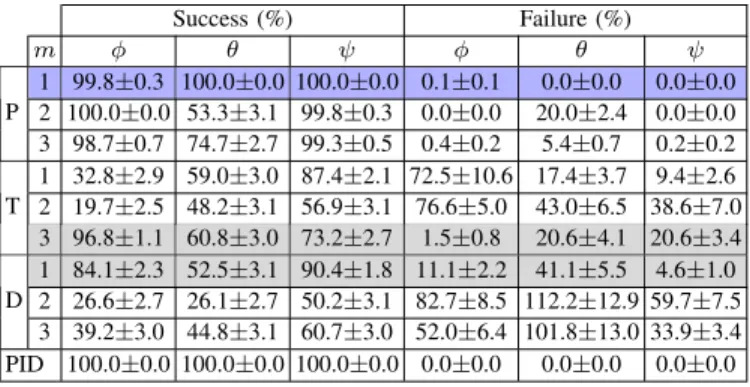
TABLE II: Success and Failure results for considered algo-rithms. P=PPO, T=TRPO, and D=DDPG. The row highlighted in blue refers to our best-performing learning agent PPO, while the rows with gray highlight correspond to the best agents for the other two algorithms.
Success (%) Failure (%) m φ θ ψ φ θ ψ P 1 99.8±0.3 100.0±0.0 100.0±0.0 0.1±0.1 0.0±0.0 0.0±0.0 2 100.0±0.0 53.3±3.1 99.8±0.3 0.0±0.0 20.0±2.4 0.0±0.0 3 98.7±0.7 74.7±2.7 99.3±0.5 0.4±0.2 5.4±0.7 0.2±0.2 T 1 32.8±2.9 59.0±3.0 87.4±2.1 72.5±10.6 17.4±3.7 9.4±2.6 2 19.7±2.5 48.2±3.1 56.9±3.1 76.6±5.0 43.0±6.5 38.6±7.0 3 96.8±1.1 60.8±3.0 73.2±2.7 1.5±0.8 20.6±4.1 20.6±3.4 D 1 84.1±2.3 52.5±3.1 90.4±1.8 11.1±2.2 41.1±5.5 4.6±1.0 2 26.6±2.7 26.1±2.7 50.2±3.1 82.7±8.5 112.2±12.9 59.7±7.5 3 39.2±3.0 44.8±3.1 60.7±3.0 52.0±6.4 101.8±13.0 33.9±3.4 PID 100.0±0.0 100.0±0.0 100.0±0.0 0.0±0.0 0.0±0.0 0.0±0.0
and that also it accumulates higher rewards. What is also interesting and counter-intuitive is that the larger memory size actuallydecreasesconvergence and stability among all trained algorithms. Recall from Section II that RL algorithms learn a policy to map states to action. A reason for the decrease in convergence could be attributed to the state space increasing causing the RL algorithm to take longer to learn the mapping to the optimal action. As part of our future work, we plan to investigate using separate memory sizes for the error and rotor velocity to decrease the state space. Reward gains during training of TRPO and DDPG are quite inconsistent with large confidence intervals. Learning performance is comparable to that observed in[8], where TRPO is able to accumulate more reward than DDPG during training for the task of navigation control.
Each trained agent was then evaluated on 1,000 never before seen command inputs in an episodic task. Since there are
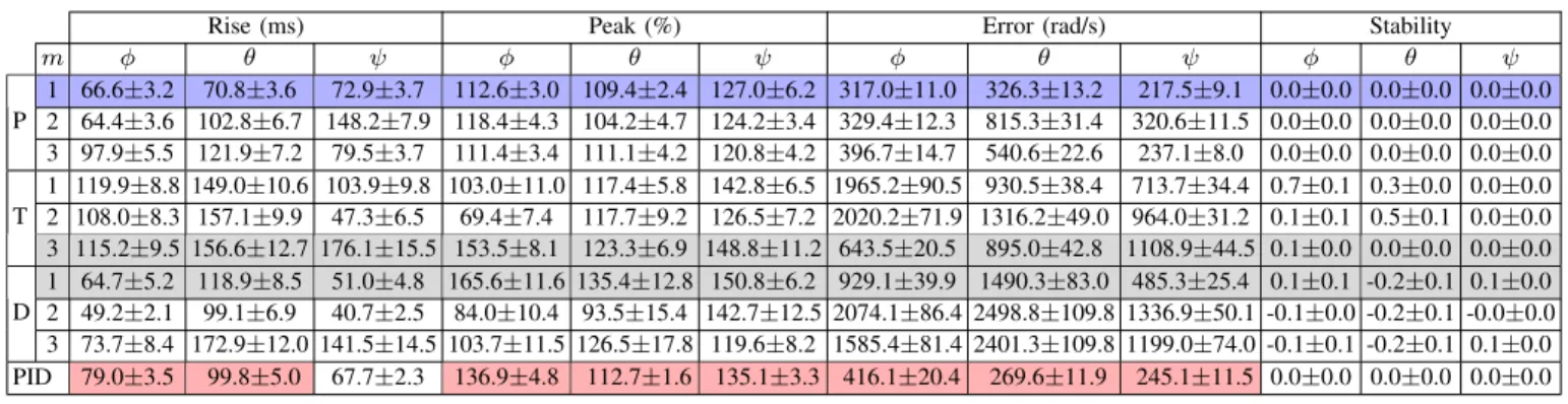
TABLE III: RL performance evaluation compared to PID of best-performing agent. Values reported are the average of 1,000 command inputs with 95% confidence where P=PPO, T=TRPO, and D=DDPG. PPOm= 1highlighted in blue outperforms all other agents, including PID control. Metrics highlighted in red for PID control are outpreformed by the PPO agent.
Rise (ms) Peak (%) Error (rad/s) Stability
m φ θ ψ φ θ ψ φ θ ψ φ θ ψ P 1 66.6±3.2 70.8±3.6 72.9±3.7 112.6±3.0 109.4±2.4 127.0±6.2 317.0±11.0 326.3±13.2 217.5±9.1 0.0±0.0 0.0±0.0 0.0±0.0 2 64.4±3.6 102.8±6.7 148.2±7.9 118.4±4.3 104.2±4.7 124.2±3.4 329.4±12.3 815.3±31.4 320.6±11.5 0.0±0.0 0.0±0.0 0.0±0.0 3 97.9±5.5 121.9±7.2 79.5±3.7 111.4±3.4 111.1±4.2 120.8±4.2 396.7±14.7 540.6±22.6 237.1±8.0 0.0±0.0 0.0±0.0 0.0±0.0 T 1 119.9±8.8 149.0±10.6 103.9±9.8 103.0±11.0 117.4±5.8 142.8±6.5 1965.2±90.5 930.5±38.4 713.7±34.4 0.7±0.1 0.3±0.0 0.0±0.0 2 108.0±8.3 157.1±9.9 47.3±6.5 69.4±7.4 117.7±9.2 126.5±7.2 2020.2±71.9 1316.2±49.0 964.0±31.2 0.1±0.1 0.5±0.1 0.0±0.0 3 115.2±9.5 156.6±12.7 176.1±15.5 153.5±8.1 123.3±6.9 148.8±11.2 643.5±20.5 895.0±42.8 1108.9±44.5 0.1±0.0 0.0±0.0 0.0±0.0 D 1 64.7±5.2 118.9±8.5 51.0±4.8 165.6±11.6 135.4±12.8 150.8±6.2 929.1±39.9 1490.3±83.0 485.3±25.4 0.1±0.1 -0.2±0.1 0.1±0.0 2 49.2±2.1 99.1±6.9 40.7±2.5 84.0±10.4 93.5±15.4 142.7±12.5 2074.1±86.4 2498.8±109.8 1336.9±50.1 -0.1±0.0 -0.2±0.1 -0.0±0.0 3 73.7±8.4 172.9±12.0 141.5±14.5 103.7±11.5 126.5±17.8 119.6±8.2 1585.4±81.4 2401.3±109.8 1199.0±74.0 -0.1±0.1 -0.2±0.1 0.1±0.0 PID 79.0±3.5 99.8±5.0 67.7±2.3 136.9±4.8 112.7±1.6 135.1±3.3 416.1±20.4 269.6±11.9 245.1±11.5 0.0±0.0 0.0±0.0 0.0±0.0
2 agents per configuration, each configuration was evaluated over a total of 2,000 episodes. The average performance metrics for Rise, Peak, Error and Stability for the response to the 2,000 command inputs is reported in Table I. Results show that the agent trained with PPO outperforms TRPO and DDPG in every measurement. In fact, PPO is the only one that is able to achieve stability (for everym), while all other agents have at least one axis where the Stability metrics is non-zero.
Next the best performing agent for each algorithm and memory size is compared to the PID controller. The best agent was selected based on the lowest sum of errors of all three axis reported by the Error metric. The Success and Failure metrics are compared in Table II. Results show that agents trained with PPO would be the only ones good enough for flight, with a success rate close to perfect, and where the roll failure of0.2%
is only off by about0.1%from the setpoint. However the best trained agents for TRPO and DDPG are often significantly far away from the desired angular velocity. For example TRPO’s best agent,39.2%of the time does not reach the desired pitch target with upwards of a20% error from the setpoint.
Next we provide our thorough analysis comparing the best agents in Table III. We have found that RL agents trained with PPO using m = 1 provide performance and accuracy exceeding that of our PID controller in regards to rise time, peak velocities achieved, and total error. What is interesting is that usually a fast rise time could cause overshoot however the PPO agent has on average a faster rise time and less overshoot. Both PPO and PID reach a stable state measured halfway through the simulation.
To illustrate the performance of each of the best agents a random simulation is sampled and the step response for each attitude command is displayed in Figure 5 along with the target angular velocity to achieve Ω∗. All algorithms reach some
steady state however only PPO and PID do so within the error band indicated by the dashed red lines. TRPO and DDPG have extreme oscillations in both the roll and yaw axis, which would cause disturbances during flight. To highlight the performance and accuracy of the PPO agent we sample another simulation and show the step response and also the PWM control signals
generated by each controller in Figure 6. In this figure we can see the PPO agent has exceptional tracking capabilities of the desired attitude. The PPO agent has a 2.25 times faster rise time on the roll axis, 2.5 times faster on the pitch axis and 1.15 time faster on the yaw axis. Furthermore the PID controller experiences slight overshoot in both the roll and yaw axis while the PPO agent does not. In regards to the control output, the PID controller exerts more power to motor three but then motor values eventually level off while the PPO control signal oscillates comparably more.
VI. FUTUREWORK ANDCONCLUSION
In this paper we presented our RL training environment GYM FC for developing intelligent attitude controllers for UAVs. We placed an emphasis on digital twinning concepts to allow transferability to real hardware. We used GYMFC to evaluate the performance of state-of-the-art RL algorithms PPO, TRPO and DDPG to identify if they are appropriate to synthesize high-precision attitude flight controllers. Our results highlight that: (i) RL can train accurate attitude controllers; and (ii) that those trained with PPO outperformed a fully tuned PID controller on almost every metric. Although we base our evaluation on results obtained in episodic tasks, we found that trained agents were able to perform exceptionally well also in continuous tasks without retraining (Appendix A). This suggests that training using episodic tasks is sufficient for developing intelligent attitude controllers. The results pre-sented in this work can be considered as a first milestone and a good motivation to further inspect the boundaries of RL for intelligent control. With this premise, we plan to develop our future work along three main avenues. On the one hand, we plan to investigate and harness the true power of RL’s ability to adapt and learn in environments with dynamic properties (e.g. wind, variable payload). On the other hand we intend to transfer our trained agents onto a real aircraft to evaluate their live performance. Furthermore, we plan to expand GYMFC to support other aircraft such as fixed wing, while continuing to increase the realism of the simulated environment by improving the accuracy of our digital twins.
0 1 2 Roll (rad/s) Ω∗φ PPO PID TRPO DDPG −4 −2 0 Pitch (rad/s) Ω∗ θ PPO PID TRPO DDPG 0.0 0.2 0.4 0.6 0.8 1.0 Time (s) −2 −1 0 Y aw (rad/s) Ω∗ ψ PPO PID TRPO DDPG
Fig. 5: Step response of best trained RL agents compared to PID. Target angular velocity isΩ∗ = [2.20,
−5.14,−1.81] rad/s shown by dashed black line. Error bars ±10% of initial error fromΩ∗ are shown in dashed red.
0 2 Roll (rad/s) Ω∗ φ PPO PID −1 0 Pitch (rad/s) Ω∗ θ PPO PID 0.0 2.5 5.0 Y aw (rad/s) Ω∗ψ PPO PID 0.0 0.2 0.4 0.6 0.8 1.0 Time (s) 0 500 1000 PWM V alues PPO-M0 PPO-M1 PPO-M2 PPO-M3 PID-M0 PID-M1 PID-M2 PID-M3
Fig. 6: Step response and PWM motor signals of the best trained PPO agent compared to PID. Target angular velocity is
Ω∗= [2.11,
REFERENCES
[1] K. N. Maleki, K. Ashenayi, L. R. Hook, J. G. Fuller, and N. Hutchins, “A reliable system design for nondeterministic adaptive controllers in small uav autopilots,” inDigital Avionics Systems Conference (DASC), 2016 IEEE/AIAA 35th. IEEE, 2016, pp. 1–5.
[2] F. Santoso, M. A. Garratt, and S. G. Anavatti, “State-of-the-art intelligent flight control systems in unmanned aerial vehicles,”IEEE Transactions on Automation Science and Engineering, 2017.
[3] O. Miglino, H. H. Lund, and S. Nolfi, “Evolving mobile robots in simulated and real environments,”Artificial life, vol. 2, no. 4, pp. 417– 434, 1995.
[4] T. Dierks and S. Jagannathan, “Output feedback control of a quadrotor uav using neural networks,” IEEE transactions on neural networks, vol. 21, no. 1, pp. 50–66, 2010.
[5] A. Bobtsov, A. Guirik, M. Budko, and M. Budko, “Hybrid parallel neuro-controller for multirotor unmanned aerial vehicle,” inUltra Mod-ern Telecommunications and Control Systems and Workshops (ICUMT), 2016 8th International Congress on. IEEE, 2016, pp. 1–4.
[6] J. F. Shepherd III and K. Tumer, “Robust neuro-control for a micro quadrotor,” inProceedings of the 12th annual conference on Genetic and evolutionary computation. ACM, 2010, pp. 1131–1138. [7] P. S. Williams-Hayes, “Flight test implementation of a second generation
intelligent flight control system,” infotech@ Aerospace, AIAA-2005-6995, pp. 26–29, 2005.
[8] J. Hwangbo, I. Sa, R. Siegwart, and M. Hutter, “Control of a quadrotor with reinforcement learning,”IEEE Robotics and Automation Letters, vol. 2, no. 4, pp. 2096–2103, 2017.
[9] “Iris Quadcopter,” 2018. [Online]. Available: http://www.arducopter.co. uk/iris-quadcopter-uav.html
[10] G. Brockman, V. Cheung, L. Pettersson, J. Schneider, J. Schul-man, J. Tang, and W. Zaremba, “Openai gym,” arXiv preprint arXiv:1606.01540, 2016.
[11] T. Gabor, L. Belzner, M. Kiermeier, M. T. Beck, and A. Neitz, “A simulation-based architecture for smart cyber-physical systems,” in Au-tonomic Computing (ICAC), 2016 IEEE International Conference on. IEEE, 2016, pp. 374–379.
[12] W. Koch, “GymFC,” https://github.com/wil3/gymfc, 2018.
[13] S. Bouabdallah, P. Murrieri, and R. Siegwart, “Design and control of an indoor micro quadrotor,” in Robotics and Automation, 2004. Proceedings. ICRA’04. 2004 IEEE International Conference on, vol. 5. IEEE, 2004, pp. 4393–4398.
[14] N. Koenig and A. Howard, “Design and use paradigms for gazebo, an open-source multi-robot simulator,” inIntelligent Robots and Systems, 2004.(IROS 2004). Proceedings. 2004 IEEE/RSJ International Confer-ence on, vol. 3. IEEE, pp. 2149–2154.
[15] V. Mnih, K. Kavukcuoglu, D. Silver, A. Graves, I. Antonoglou, D. Wier-stra, and M. Riedmiller, “Playing atari with deep reinforcement learn-ing,”arXiv preprint arXiv:1312.5602, 2013.
[16] R. S. Sutton and A. G. Barto,Reinforcement learning: An introduction. MIT press Cambridge, 1998, vol. 1, no. 1.
[17] T. P. Lillicrap, J. J. Hunt, A. Pritzel, N. Heess, T. Erez, Y. Tassa, D. Silver, and D. Wierstra, “Continuous control with deep reinforcement learning,”arXiv preprint arXiv:1509.02971, 2015.
[18] J. Schulman, S. Levine, P. Abbeel, M. Jordan, and P. Moritz, “Trust region policy optimization,” inInternational Conference on Machine Learning, 2015, pp. 1889–1897.
[19] J. Schulman, F. Wolski, P. Dhariwal, A. Radford, and O. Klimov, “Prox-imal policy optimization algorithms,”arXiv preprint arXiv:1707.06347, 2017.
[20] D. J. Leith and W. E. Leithead, “Survey of gain-scheduling analysis and design,”International journal of control, vol. 73, no. 11, pp. 1001–1025, 2000.
[21] H. P. Whitaker, J. Yamron, and A. Kezer,Design of model-reference adaptive control systems for aircraft. Massachusetts Institute of Technology, Instrumentation Laboratory, 1958.
[22] N. Hovakimyan, C. Cao, E. Kharisov, E. Xargay, and I. M. Gregory, “L1 adaptive control for safety-critical systems,”IEEE Control Systems, vol. 31, no. 5, pp. 54–104, 2011.
[23] “BetaFlight,” 2018. [Online]. Available: https://github.com/betaflight/ betaflight
[24] M. Fatan, B. L. Sefidgari, and A. V. Barenji, “An adaptive neuro pid for controlling the altitude of quadcopter robot,” inMethods and models in automation and robotics (mmar), 2013 18th international conference on. IEEE, 2013, pp. 662–665.
[25] S. L. Waslander, G. M. Hoffmann, J. S. Jang, and C. J. Tomlin, “Multi-agent quadrotor testbed control design: Integral sliding mode vs. reinforcement learning,” inIntelligent Robots and Systems, 2005.(IROS 2005). 2005 IEEE/RSJ International Conference on. IEEE, 2005, pp. 3712–3717.
[26] N. Jakobi, P. Husbands, and I. Harvey, “Noise and the reality gap: The use of simulation in evolutionary robotics,” Advances in artificial life, pp. 704–720, 1995.
[27] “Protocol Buffers,” 2018. [Online]. Available: https://developers.google. com/protocol-buffers/
[28] “ArduPilot,” 2018. [Online]. Available: http://ardupilot.org/
[29] “gzserver doesn’t close disconnected sockets,” 2018. [Online]. Available: https://bitbucket.org/osrf/gazebo/issues/2397/ gzserver-doesnt-close-disconnected-sockets
[30] A. Karpathy, “Deep Reinforcement Learning: Pong from Pixels,” 2018. [Online]. Available: http://karpathy.github.io/2016/05/31/rl/
[31] P. Dhariwal, C. Hesse, O. Klimov, A. Nichol, M. Plappert, A. Radford, J. Schulman, S. Sidor, and Y. Wu, “Openai baselines,” https://github. com/openai/baselines, 2017.
[32] J. G. Ziegler and N. B. Nichols, “Optimum settings for automatic controllers,”trans. ASME, vol. 64, no. 11, 1942.
APPENDIXA
CONTINUOUSTASKEVALUATION
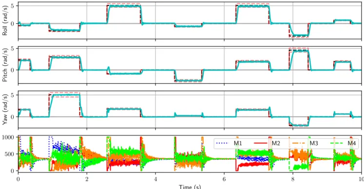
In this section we briefly expand on our findings that show that even if agents are trained through episodic tasks their performance transfers to continuous tasks without the need for additional training. Figure 7 shows that an agent trained with Proximal Policy Optimization (PPO) using episodic tasks has exceptional performance when evaluated in a continuous task. Figure 8 is a close up of another continuous task sample showing the details of the tracking and corresponding motor output. These results are quite remarkable as they suggest that training with episodic tasks is sufficient for developing intelli-gent attitude flight controller systems capable of operating in a continuous environment. In Figure 9 another continuous task is sampled and the PPO agent is compared to a PID agent. The performance evaluation shows the PPO agent to have 22% decrease in overall error in comparison to the PID agent.
−5 0 5 Roll (rad/s) −5 0 5 Pitch (rad/s) 0 10 20 30 40 50 60 Time (s) −5 0 5 Y aw (rad/s)
Fig. 7: Performance of PPO agent trained with episodic tasks but evaluated using a continuous task for a duration of 60 seconds. The time in seconds at which a new command is issued is randomly sampled from the interval [0.1,1] and each issued command is maintained for a random duration also sampled from [0.1,1]. Desired angular velocity is specified by the black line while the red line is the attitude tracked by the agent.
0 5 Roll (rad/s) 0 5 Pitch (rad/s) 0 5 Y aw (rad/s) 0 2 4 6 8 10 Time (s) 0 500 1000 PWM V alues M1 M2 M3 M4
![Fig. 5: Step response of best trained RL agents compared to PID. Target angular velocity is Ω ∗ = [2.20, −5.14, −1.81] rad/s shown by dashed black line](https://thumb-us.123doks.com/thumbv2/123dok_us/1363626.2682555/11.918.137.770.153.478/response-trained-agents-compared-target-angular-velocity-dashed.webp)