Air Force Institute of Technology
AFIT Scholar
Theses and Dissertations Student Graduate Works
3-22-2012
Using QR Factorization for Real-Time Anomaly
Detection of Hyperspectral Images
Kelly R. Bush
Follow this and additional works at:https://scholar.afit.edu/etd Part of theOther Electrical and Computer Engineering Commons
USING QR FACTORIZATION FOR REAL-TIME ANOMALY DETECTION OF HYPERSPECTRAL IMAGES
THESIS
Kelly R. Bush
AFIT-OR-MS-ENS-12-04
DEPARTMENT OF THE AIR FORCE AIR UNIVERSITY
AIR FORCE INSTITUTE OF TECHNOLOGY
Wright-Patterson Air Force Base, Ohio
The views expressed in this thesis are those of the author and do not reflect the official policy or position of the United States Air Force, Department of Defense, or the United States Government.
AFIT-OR-MS-ENS-12-04
USING QR FACTORIZATION FOR REAL-TIME ANOMALY DETECTION OF HYPERSPECTRAL IMAGES
THESIS
Presented to the Faculty Department of Operations Research
Graduate School of Engineering and Management Air Force Institute of Technology
Air University
Air Education and Training Command In Partial Fulfillment of the Requirements for the Degree of Master of Science in Operations Research
Kelly R. Bush, BS USAF Civilian GS-11
March 2012
AFIT-OR-MS-ENS-12-04
USING QR FACTORIZATION FOR REAL-TIME ANOMALY DETECTION OF HYPERSPECTRAL IMAGES
Kelly R. Bush, BS USAF Civilian GS-11
Approved:
___________________________________ __________
Dr. Kenneth W. Bauer (Chairman) Date
___________________________________ __________
Abstract
Anomaly detection has been used successfully on hyperspectral images for over a decade. However, there is an ever increasing need for real-time anomaly detectors. Historically, anomaly detection methods have focused on analysis after the entire image has been collected. As useful as post-collection anomaly detection is, there is a great advantage to detecting an anomaly as it is being collected.
This research is focused on speeding up the process of detection for a pre-existing method, Linear RX, which is a variation on the traditional Reed-Xiaoli detector. By speeding up the process of detection, it is possible to create a real-time anomaly detector. The window covariance matrix is our main area focus for speed improvement. Several methods were investigated, including QR factorization and tracking the change in the window covariance matrix as it moves through the image. Finally, performance comparisons are made to the original Linear RX detector.
Acknowledgments
First, I would like to thank all my family and friends for supporting me in this endeavor. I am sure they have heard much more than they would like about anomaly detection in hyperspectral images. Thank you for putting up with my thesis chatter.
I would also like to thank my thesis advisor, Dr. Kenneth Bauer, and my reader, Lt Col Mark Friend, for their continued support and confidence in me. Last, but certainly not least, I would like to thank Capt Jason Williams and Mr. Trevor Bihl for answering so many of my questions.
Table of Contents
Page
Abstract ... iii
Acknowledgments... iv
Table of Contents ...v
List of Figures ... vii
List of Tables ... ix List of Equations ...x 1. Introduction ...1 1.1 General Issue ...1 1.2 Methodology ...1 1.3 Preview ...2 2. Literature Review...3 2.1 HSI Basics ...3 2.2 Anomaly Detection ...6 2.2.1 Reed-Xiaoli (RX) Detector ... 9 2.2.2 Linear RX Detector ... 10 2.2.3 Real-time Detectors ... 11
2.3 Principal Components Analysis ...14
2.4 QR Factorization ...15
2.5 Performance Measurements ...16
3.0 Methodology ...18
3.1 Chapter Overview ...18
3.2 Algorithm Development...18
3.2.1 Changes to the Linear RX Anomaly Detector ... 19
3.2.2 Assumption for Principal Components Analysis ... 21
3.2.3 Decreasing the Number of Covariance Matrix Changes ... 22
3.3 Experimental Design ...23
3.4 HYDICE Hyperspectral Images ...24
3.5 Summary ...25
4.2 Tracking the Covariance Matrix Changes...26
4.3 Finding the Best Settings ...29
4.4 Time Savings ...30
4.5 Accuracy ...30
4.6 Summary ...34
5. Conclusions and Recommendations ...35
5.1 Chapter Overview ...35
5.2 Conclusions of Research ...35
5.3 Recommendations for Future Research ...35
5.3.1 Proposed Process for Situation that Violate the Assumptions ... 35
5.3.2 Trace of the Covariance Matrix ... 36
5.3.3 Step Changes to the Covariance Matrix ... 36
Appendix A ...37
Appendix B ...42
Bibliography ...43
List of Figures
Page
Figure 1: Electromagnetic Spectrum. Reprinted from (Landgrebe D. A., 2003) ... 4
Figure 2: Illustration of Matrices within an Image Cube. Reprinted from (Miller, 2009) . 5 Figure 3: “Pushbroom” Data Collection. Reprinted from (Bihl) ... 6
Figure 4: RX Moving Window. Reprinted from (Williams, Bihl, & Bauer)... 9
Figure 5: LRX Moving Column. Reprinted from (Williams, Bihl, & Bauer) ... 11
Figure 6: Confusion Matrix. Adapted from (Fawcett, 2006) ... 16
Figure 7: Direction of Data Collection Assumption ... 19
Figure 8: Illustration of the Issue with PCA in Real-Time Detection ... 22
Figure 9: ARES 2D Image and Mapping of Pixels with a Large Trace Difference ... 28
Figure 10: ARES 3F Image and Mapping of Pixels with a Large Trace Difference ... 28
Figure 11: ROC Comparison of Methods on ARES 3D ... 32
Figure 12: ROC Comparison of Methods on ARES 4 ... 32
Figure 13: ROC Comparison of Methods on ARES 5 ... 33
Figure 14: ROC Comparison of Methods on ARES 5D 20kFT ... 33
Figure 15: Color Image for ARES 1D ... 37
Figure 16: Color Image for ARES 1F ... 37
Figure 17: Color Image for ARES 2D ... 38
Figure 18: Color Image for ARES 2F ... 38
Figure 19: Color Image for ARES 3D ... 39
Figure 22: Color Image for ARES 4F ... 40 Figure 23: Color Image for ARES 5 ... 41 Figure 24: Color Image for ARES 5D_20kFT ... 41
List of Tables
Page
Table 1: Settings Tested for Optimal Model Accuracy ... 23
Table 2: Details on the HYDICE Training Images ... 24
Table 3: Details on the HYDICE Test Images... 25
Table 4: Histogram of the Differences in the Trace for ARES 1F ... 27
List of Equations Page Equation 1 ... 8 Equation 2 ... 9 Equation 3 ... 12 Equation 4 ... 12 Equation 5 ... 12 Equation 6 ... 12 Equation 7 ... 12 Equation 8 ... 13 Equation 9 ... 13 Equation 10 ... 14 Equation 11 ... 15 Equation 12 ... 20 Equation 13 ... 20 Equation 14 ... 20 Equation 15 ... 20 Equation 16 ... 20 Equation 17 ... 21
REAL-TIME ANOMALY DETECTION OF HYPERSPECTRAL IMAGES
1. Introduction
1.1 General Issue
As sensor technology advances, the amount of data produced is ever increasing. This massive amount of data makes anomaly detection by human eyes alone virtually impossible. Anomaly detection by humans alone is also impractical, since the human eye can be tricked by methods such as camouflage. Because of this, anomaly detection methods are being created to help analyze images in an accurate and timely manner.
Historically, anomaly detection methods have focused on analysis after the entire image has been collected. As useful as post-collection anomaly detection is, there is a great advantage to detecting an anomaly as the data is being collected. The faster an anomaly is detected, the sooner something can be done about it. By speeding up the process of detection, it is within the realm of possibility to create an anomaly detector that works in real-time.
1.2 Methodology
One common anomaly detector is the RX detector (Reed & Yu, 1990). This detector decides whether each pixel is a statistical anomaly or not by comparing a pixel’s score to a statistical value. This pixel’s score is computed using an inverse covariance matrix. Linear RX (Williams, Bihl, & Bauer) is another anomaly detector that uses a similar technique of scoring using an inverse covariance matrix. It is well known that taking the inverse of a large matrix, like a covariance matrix, can be very computationally
2001) and (Du & Zhang, 2011) that by using QR factorization, the inverse of a
covariance matrix can be found in a more timely manner. In this research, we will show that QR factorization can indeed speed up Linear RX and that the qualities of Linear RX can be taken advantage of in a real-time processing setting.
1.3 Preview
Chapter 2 explains some of the basics of hyperspectral images and anomaly detection. It also contains information on some current real-time anomaly detectors as well as the concepts used in the implementation and analysis of this research. Chapter 3 details how QR factorization is implemented in order to speed up the detection process. Chapter 4 includes the analysis and results of this new method. Finally, Chapter 5
provides an overview of the work completed in this paper as well as recommendations for future work.
2. Literature Review
This chapter outlines current practices in hyperspectral imaging (HSI) and anomaly detection as well as mathematical methods used in this thesis. This chapter is organized into six sections: HSI basics, Anomaly Detection, Principal Components Analysis, Normalized Difference Vegetation Index, QR Factorization, and Performance Measurements.
2.1 HSI Basics
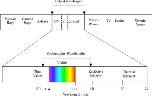
All images capture some portion of the electromagnetic (EM) spectrum. Images taken with a common digital camera capture the visible portion of the EM spectrum in three discrete wavelength bands: red, green and blue. In a similar manner, multispectral images capture discrete wavelength bands, but feature multiple bands across several EM regions. Hyperspectral images are similar in concept to multispectral images except for some key differences. One of the main differences is that instead of capturing discrete wavelength bands, hyperspectral images capture a finely sampled contiguous region of the EM spectrum, which is then broken down into many bands. Hyperspectral images are comprised of 20 or more wavelength bands (Stein, Beaven, Hoff, Winter, Schaum, & Stocker, 2002). Figure 1 illustrates the EM spectrum and the various regions of the spectrum.
Figure 1: Electromagnetic Spectrum. Reprinted from (Landgrebe D. A., 2003)
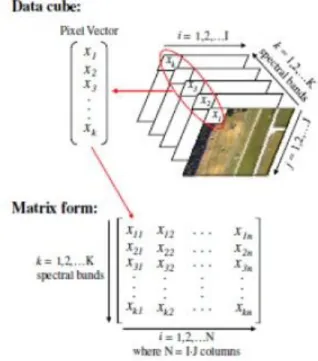
All of this information must be properly organized and the two aspects of the data that must be captured: spatial location and the spectral wavelength band. Typically the hyperspectral image data is organized into an ‘image cube’ (Smeteck & Bauer, 2008). This 3-dimensional data array has height m, width n, and spectral k dimensions. In this way, the spatial location is recorded as a pixel, using the height and width dimensions, and the spectral wavelength band is captured in the third dimension. This image cube can be thought of as a stack of k images of size mxn, where each image is a representation of the same physical area, but on different spectral bands. Figure 2 demonstrates this concept.
Figure 2: Illustration of Matrices within an Image Cube. Reprinted from (Miller, 2009)
Hyperspectral imaging is a powerful tool because it takes advantage of the fact that different materials reflect, absorb and emit electromagnetic energy differently due to each material’s molecular composition (Manolakis & Shaw, 2002), (Eismann, 2011). Theoretically each material has a unique reflection and radiation pattern, which is sometimes called a material’s spectral signature. Because of this, different materials can be identified by their spectral signature. For example, trees will reflect and radiate electromagnetic energy differently than a parking lot and therefore will have a different spectral signature. By capturing these spectral signatures, HSI is useful in a variety of applications ranging from environmental monitoring to surveillance (Stein, Beaven, Hoff, Winter, Schaum, & Stocker, 2002).
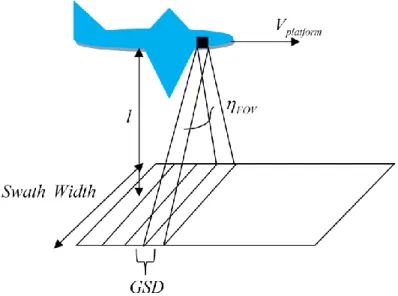
This paper will assume that the HSI data is collected from a “push broom” sensor. This type of sensor collects data one line at a time as the sensor platform (i.e. satellite, plane, or UAV) flies over the area of interest.
Figure 3: “Pushbroom” Data Collection. Reprinted from (Bihl)
2.2 Anomaly Detection
Anomaly detection and recognition are relatively common applications of HSI. There are two general types of detectors: anomaly detection algorithms and signature matching algorithms (Stein, Beaven, Hoff, Winter, Schaum, & Stocker, 2002), (Eismann, 2011). Signature matching algorithms require a priori information on what type of material the detector is searching for. This can prove difficult, since the type of target is
statistically different from the background of the image (Eismann, 2011), (Stein, Beaven, Hoff, Winter, Schaum, & Stocker, 2002). It is important to note that these detectors only find anomalous objects; they do not classify its spectral signature. For example, if there is a building in the middle of a field, an anomaly detector might recognize the building as an anomaly, but would not know that it is a building. However, if the image contains many buildings, parking lots, and streets, then the detector may recognize the buildings as background and grass growing in a sidewalk crack as an anomaly.
Hyperspectral images are better suited for anomaly detection than a common RGB image. This is due to the multiple spectral bands within which an anomaly could be detected. Suppose there is a field and in the middle of this field there is a crate disguised with camouflage. If we run an anomaly detection algorithm on an RGB image of this field, an anomaly may not be detected. The camouflage could almost completely disguise the crate in the RGB image, but it would not be so easily hidden in a hyperspectral image of the field. The anomaly may be detected on a different spectral band, say in the infrared region, which is not captured in the RGB image, where water absorption properties would be noticeably different between the camouflage and vegetation in the field. This is why HSI is more effective at detecting anomalies than common RGB images.
There are three types of anomaly detection techniques: supervised,
semi-supervised, and unsupervised. Training data of both the background and the anomaly is needed for supervised detection. Semi-supervised detection only requires training data of the background. As for unsupervised detection, no training data is required, just as the name suggests. Depending on the situation, supervised and semi-supervised detection can
to image. Because of this, it is difficult to train a detector on one image and use it on another with good results.
There are two main approaches to defining the background of the image: local and global. Global anomaly detection defines background as the entire image excluding the test pixel. Therefore, global methods compare a given test pixel to the rest of the image. Local anomaly detection defines background as a smaller subset of the image. Usually, it compares the test pixel to a window of pixels around the test pixel. Both methods have their advantages. Global anomaly detection is less susceptible to false alarms than local anomaly detection. On the other hand, local anomaly detection is better at finding an isolated target that resembles background (Stein, Beaven, Hoff, Winter, Schaum, & Stocker, 2002), (Smeteck & Bauer, 2008).
One common method used to find pixels that are statistically different from the background is to measure the Mahalanobis distance between the pixel and the mean vector of the background (Eismann, 2011). This distance is defined as:
Equation 1 (1)
where is the test pixel, is the mean vector of the background, and is the covariance matrix of the background (Dillon & Goldstein, 1984). When compared to Euclidean distance, Mahalanobis distance has the distinct advantage of accounting for any
2.2.1 Reed-Xiaoli (RX) Detector
The Reed-Xiaoli (RX) detector, introduced by Reed and Yu (Reed & Yu, 1990), is an unsupervised local anomaly detector based on the Mahalanobis distance. Using a moving window, the RX detector identifies anomalies by comparing the center pixel to the rest of the pixels in the window, as illustrated in Figure 4. This center pixel is given a score based on a generalized likelihood ratio test. After a pixel has been tested, the window is moved across each row, one pixel at a time.
Figure 4: RX Moving Window. Reprinted from (Williams, Bihl, & Bauer)
The RX detector assumes Gaussian data and uses the following Equation 2 as the pixel score
Equation
2
(2)
RX(x) score is greater than , then x is considered an anomaly. Note that as the window size, N, gets larger, the RX score approaches the Mahalanobis distance.
Choosing an appropriately sized window for the RX detector can prove difficult. If the window is too restrictive, the detector will not pick up on large anomalies because the majority of the window is filled with the pixels of that anomaly. If the window is too large, the window could contain several anomalies and the representation of the original background is corrupted. Because of this, it is important to set the window size based on what sized target you want to detect. Variations of RX exist to counteract pixel spatial proximity issues. These methods include applying a guard window around a test pixel, so that pixels immediately surrounding the test pixel are not included in the background calculation (Eismann, 2011), and different geometric window shapes in order to increase the spatial distance of the pixels used to calculate the background (Williams, Bihl, & Bauer).
2.2.2 Linear RX Detector
Linear RX (LRX), developed by Williams, Bihl, and Bauer, is a variation on the classic RX detector (Williams, Bihl, & Bauer). Instead of using a moving window around the test pixel, LRX looks at a line of pixels above and below the test pixels. If there are insufficient pixels above or below the test pixel, the remaining pixels are taken from the bottom of the previous column or the top of the next column, respectively, as shown in
Figure 5: LRX Moving Column. Reprinted from (Williams, Bihl, & Bauer)
LRX was created to address the issue of pixel correlation based on spatial
proximity (Williams, Bihl, & Bauer). For example, a large anomaly that is about the size of the RX window will not be picked up by the standard RX detector. However, the LRX will recognize it as an anomaly since it is comparing the test pixel to pixels across a wide range of the image. The use of a line of pixels in place of a window increases the average distance between the pixels, which allows for reduction of bias and error in the estimation of the mean vector and covariance matrix (Williams, Bihl, & Bauer).
2.2.3 Real-time Detectors
There is an ever increasing need for real-time anomaly detection methods (Du & Zhang, 2011). We use the term “real-time” loosely, since there really is no definition of what makes a detection method real-time. For our purposes, if the detection method can be carried out while new rows of data are added and it is at least as fast as current
post-There are two current real-time detectors that will be used for comparison for this paper. Both are presented in Stellman et al. (Stellman, Hazel, Bucholtz, Michalowicz, Stocker, & Schaaf, 2000).
The first detector is a real-time version of the RX algorithm. Each time there is new data, a new mean vector µ and a new covariance matrix S are calculated using Equation 3 and Equation 4 respectively. Note that the contribution of the new pixel is weighted by α as defined by Equation 5.
Equation 3 (3)
Equation 4 (4)
Equation 5
(5)
where, is the vector of spectral components for the nth pixel and is the sample
average (Stellman, Hazel, Bucholtz, Michalowicz, Stocker, & Schaaf, 2000). The inverse covariance matrix is calculated by:
Equation6 (6)
where, E is a matrix of the eigenvectors of the covariance matrix with the form with j as the number of spectral bands (Stellman, Hazel, Bucholtz,
Equation
8
(8)
where, represents the ith element of the principal component and is the associated eigenvalue.
For the second real-time anomaly detection algorithm, we will use a clustering algorithm defined in (Stellman, Hazel, Bucholtz, Michalowicz, Stocker, & Schaaf, 2000). This clustering algorithm is a semi-supervised detection method, therefore it requires a training set of background data. The algorithm looks at N frames of sensor data and each new frame of data replaces the oldest frame. The training set is used as the initial N frames which are then divided into C clusters. Then each pixel has the mean vector of its cluster subtracted from it and a covariance matrix is computed for the centered pixels. As new frames of data are included, the algorithm separates the new pixels into the pre-constructed clusters, by finding the cluster whose mean is closest to that pixel. This can also be stated as:
Equation 9 (9)
where cn is the cluster to which the nth pixel, zn, is assigned and mi is the mean of the ith
Once all of the new pixels have been assigned to a cluster, the mean of each cluster is recalculated. Each pixel in the new frame is then centered and the covariance matrix is updated, using Equation 10:
Equation 10
(10)
where is the jth update of the covariance matrix, is the number of frames included, is the number of pixels in a frame, and is the centered ith pixel.
2.3 Principal Components Analysis
There are many constraints on the storage and analysis of HSI data. For example, the storage capability of onboard systems may be limited for the un-manned vehicle (UAV), helicopter, or airplane that is collecting the data. Also, much of the analysis is carried out on commercial off-the-shelf (COTS) computers (Farrell & Mersereau, 2005). Because of these limitations, it is common practice to conduct a data reduction technique, such as principal components analysis (PCA) (Gu, Liu, & Zhang, 2006), (Farrell & Mersereau, 2005). PCA is a type of multivariate statistical technique that is used to reduce the dimensionality of a set of data. Principal components are linear combination of the data’s variables (Dillon & Goldstein, 1984). The first component is created such that the greatest amount of variance in the data is captured by the linear combination while the length equals one. The second component is constructed orthogonal to the first
retained. However, it is possible to lose important knowledge contained in an image. Therefore, the goal is to explain the most variance of the original set with as few
principal components as possible. Retained principal components are then used instead of the variables in the analysis.
Applying this to HSI, principal components are found in the data cube with the spectral bands acting as the variables. By using principal components, we can achieve dimensionality reductions of approximately 90 percent, while retaining much of the variance within the data. However, it is important to retain a sufficient number of
principal components in order for anomalies, which can be a small percentage of the data, to be detected.
2.4 QR Factorization
QR factorization is one technique that can be used to help simplify matrix
computations in the RX equation. How QR factorization accomplishes this task is shown later in the paper.
A real matrix Acan be factored into two matrices: an orthogonal matrix Q and an upper or right triangular matrix R. The factorization looks like Equation 11.
Equation 11 (11)
There are several ways to compute Q and R, including the Givens rotations, Householder transformations and the Gram-Schmidt orthogonalization process (Golub & Van Loan, 1989), (Meyer, 2000).
2.5 Performance Measurements
In order to measure the performance of the anomaly detection methods, we need to look at what mistakes the methods are making. Each pixel has two possible true states, either the pixel is an anomaly or it is not. The detector also can classify each pixel as an anomaly or background. This leads to four possible states for the classification of each pixel, which are laid out in Figure 6, commonly termed a confusion matrix.
Detector Classification Anomaly Background T ru e S tat e Anomaly True Positive False Negative Background False Positive True Negative
Figure 6: Confusion Matrix. Adapted from (Fawcett, 2006)
As shown in the confusion matrix above, there are two ways the detector can be correct. If a pixel is true positive or true negative, then the detector successfully classified the true state of the pixel. However, if a pixel is false positive or false negative, then the detector classified a background pixel as an anomaly or an anomalous pixel as
background. Obviously, we are interested in a detector that has many true positives or true negatives, with very few false positives or false negatives.
number of false positives divided by the number of non-anomalies. This means the FPF is the percentage of non-anomalies that are incorrectly identified.
Receiver operating characteristic (ROC) curves are commonly used to assess the accuracy of detectors. A ROC curve is a plot of the TPF vs. FPF given some incremental change in the threshold (Fawcett, 2006). A ROC curve shows how changing the detection threshold affects how anomalies are detected. A lower threshold would give fewer false alarms, but would detect very few targets whereas a higher threshold would detect most of the targets, but would have many false positives.
In order to compare several methods, each is used with the same changes in threshold. The “northwest” rule is commonly used as a discriminator (Fawcett, 2006). That is if method A’s ROC curve is entirely to the north and/or west of method B’s ROC curve, it is said that method A dominates B. This means that no matter the threshold, method A performs better than B. This is why ROC curves are so useful to compare several detection methods.
3.0 Methodology
3.1 Chapter Overview
This chapter outlines the assumptions and process we propose in order to speed up the Linear RX detector and implement it as a real-time anomaly detector.
3.2 Algorithm Development
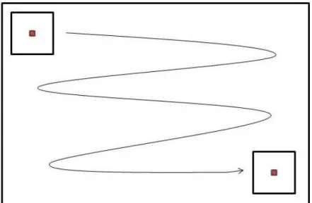
The basic idea behind our algorithm comes from the very nature of HSI data collection and the Linear RX detector. As explained in Chapter 2, HSI sensors are assumed within this research to collect hyperspectral image data using a “pushbroom” sweep of the area. Each sweep of the HSI sensor corresponds to a row of pixels. Since the LRX detector uses a line of pixels for comparison instead of a local window, the
sampling of the image mimics how the image is collected. For the purpose of this paper, we will assume that the sensor is collecting data from west to east with respect to the picture (see Figure 7). It is important to note that the original data was collected perpendicular to this direction. However, this research is using subsets of the original HYDICE imagery, so the assumed direction of collection is not important. It is also important to note that the LRX detector is sensitive to the shape of the image. Since the window is a line, the height of the image plays a key role in the average distance between the window pixels. This average distance is the key to reducing correlation due to spatial proximity.
Figure 7: Direction of Data Collection Assumption
3.2.1 Changes to the Linear RX Anomaly Detector
In order to speed up the LRX detector we decided to speed up the calculation of the inverse covariance matrix. This calculation is one area of not only the LRX detector, but many Mahalanobis based anomaly detectors that has large computation times. When working with large matrices, calculating the covariance matrix and taking the inverse can take a long time. For the LRX algorithm, over 40% of the run time is spent calculating the covariance matrix and over 25% of the run time is spent on the score calculation, which contains the covariance matrix inverse. It has been shown that the inverse
covariance matrix can be calculated faster using QR factorization in Chang et al. (Chang, Ren, & Chiang, 2001), and by Du and Zhang (Du & Zhang, 2011).
Equation 12
(12)
where S is the covariance matrix, N is the size of the window, X is an matrix of the mean corrected data from the window, an p is the number of spectral bands. Recalling Equation 12 which expressed that any matrix, can be factored through QR; Equation 13 extends this to include X
Equation 13 (13)
We can now express the covariance matrix in terms of Q and R as shown in Equation 14.
Equation 14
(14) Since Q is orthogonal, . This knowledge simplifies the equation even further as displayed in Equation 15.
Equation 15
(15)
Now we take the inverse of both sides we come up with Equation 16.
Equation 16 (16)
Even though there are still matrices to be inverted, they are upper triangular matrices and therefore easier to invert than a covariance matrix. Since we only are concerned in finding matrix R, Cholesky Decomposition is used in this research (Meyer, 2000).
matrix. Switching these two equations should not change the detection much because, as explained in chapter 2, the RX score approaches Mahalanobis distance as the window size gets larger. This assertion was tested by using Mahalanobis distance in LRX with the optimal settings set forth by Williams et al. in (Williams, Bihl, & Bauer). The ROC curves of LRX and LRX with Mahalanobis distance were exactly the same. Therefore, Mahalanobis distance is a good estimate to the RX score. After replacing the inverse covariance matrix in Equation 1 with our result in Equation 16, we have Equation 17.
Equation 17 (17)
This is the pixel score that will be used in our real-time LRX detector.
3.2.2 Assumption for Principal Components Analysis
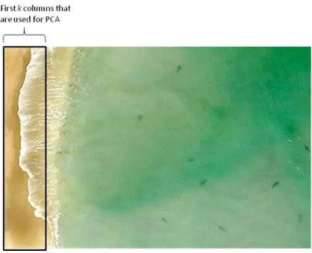
The Linear RX algorithm, as well as many detection algorithms, benefit greatly by the use of principal components analysis (PCA). This is easily done when working on an image that has already been collected, but is tricky when trying to work on an image that is in the process of being collected. Therefore, we decided to run PCA on a set number of beginning columns, say k columns, and apply the loadings across all the incoming data. One downside to this approach is if the background changes dramatically from the first k columns to later in the image, then the original PCA loadings would not represent the rest of the picture well.
For example, consider Figure 8, an image that is being collected where the left part is a sandy beach and the right part is ocean.If PCA is carried out on the first k columns and all of those columns are of the sand, then the loadings are useless in
rest of the image. In section 5.3.1, we will propose a possible solution to this problem that would require further study.
Figure 8: Illustration of the Issue with PCA in Real-Time Detection
3.2.3 Decreasing the Number of Covariance Matrix Changes
In many cases, images have a similar background throughout the entire image. This background could be a grassy plain, dessert area, or even a forest, but the point is we may not need to change our window covariance matrix every time we change the
window. If the (n+1)th window has similar data as the nth window, then we could potentially use the covariance matrix from the nth window. This could speed up the
the covariance matrix for the RX score calculation. If not, we would continue using the covariance matrix we used in the previous step.
3.3 Experimental Design
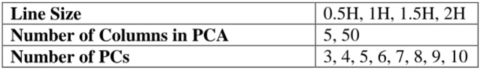
We expect that 3 factors will play a role in the detector’s accuracy: the number of pixels to include in our window (or line size), the number of initial columns to run PCA on, and the number of principal components to retain. We want line size to be scaled appropriately to the size of the image. Because there is a large range of image sizes, we will express line size in terms of the image height (H).
Table 1: Settings Tested for Optimal Model Accuracy
Line Size 0.5H, 1H, 1.5H, 2H
Number of Columns in PCA 5, 50
Number of PCs 3, 4, 5, 6, 7, 8, 9, 10
Note that if the algorithm waits for 5 columns to be collected by the sensor in order to run PCA, then by the time the analysis is started on the first pixel, the sensor has collected 5 or more columns of data. Because the largest line size we would use is 2H, we could start the analysis on the first pixel of the second column and not have any issue with our window catching up with the sensor. This of course is assuming that the sensor is just as fast as the algorithm. Since we are not concerned about the algorithm catching up with the sensor, we do not need to run a special simulation that slowly adds data to the image as the image is being analyzed. We can simply run the analysis on the entire image.
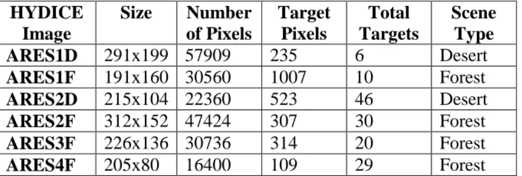
3.4 HYDICE Hyperspectral Images
This research uses several images collected by an airborne HSI Sensor called HYDICE (Hyperspectral Digital Imagery Collection Equipment). Specifically, the images come from the Forest I and Desert Radiance II canonical datasets from the HYDICE program’s 1995 data collection experiments (Eismann, 2011), (Orloff, et al., 2000).
There are two sets of images: training and test images. The training images will be used to find the optimal settings for the real-time LRX. After these optimal settings are found, the real-time LRX is used on the test images to validate the settings. Details on each image are displayed in Table 2 for the training images and in Table 3 for the test images. All of the images have 210 spectral bands and are taken from an altitude of 5,000’ AGL (Above Ground Level) except for ARES5D_20kFT. See Appendix A for true color images and truth maps.
Table 2: Details on the HYDICE Training Images
HYDICE Image Size Number of Pixels Target Pixels Total Targets Scene Type ARES1D 291x199 57909 235 6 Desert ARES1F 191x160 30560 1007 10 Forest ARES2D 215x104 22360 523 46 Desert ARES2F 312x152 47424 307 30 Forest ARES3F 226x136 30736 314 20 Forest ARES4F 205x80 16400 109 29 Forest
Table 3: Details on the HYDICE Test Images
HYDICE Image Size Number
of Pixels Target Pixels Total Targets Scene Type ARES3D 156x156 24336 438 4 Desert ARES4 460x78 35880 882 15 Desert ARES5 355x150 53250 585 15 Forest ARES5D_20kFT 139x68 9450 129 28 Desert 3.5 Summary
In this chapter, we’ve covered the development of our real-time anomaly detector, including how we intend to speed up the Linear RX detector using QR factorization to calculate the inverse covariance matrix. We’ve also covered our base assumptions, such as the direction the data is collected and that our data has similar background data throughout the image. Finally, we presented the settings we will test and the images we will use. Next, in chapter 4, we will cover the analysis and results of this research.
4. Analysis and Results
4.1 Chapter Overview
In this chapter, we will cover the analysis and results for the real-time LRX. This chapter is broken into four sections, which include tracking the covariance matrix changes, finding the best settings for the real-time LRX, time savings of the real-time LRX versus the original LRX, and the accuracy comparison between the real-time LRX and the original LRX.
4.2 Tracking the Covariance Matrix Changes
By tracking the differences in the trace of the window covariance matrix, it was anticipated to decrease the run times of the anomaly detector by eliminating many of the covariance matrix updates.
We incorporated in the algorithm a check for the change in the trace of the window covariance matrix each time the window moves to a new test pixel. After looking at the differences for one image, ARES 1F, we noticed the differences were either incredibly small or quite large. The histogram for the differences is displayed in Table 4. Note that about half the differences are less than and the other half are greater than 100. Based on this table, we implemented a rule of thumb that if the trace difference is greater than , then use the new covariance matrix in the
Table 4: Histogram of the Differences in the Trace for ARES 1F Bin Frequency 1.00E-10 15468 1.00E-08 0 1.00E-06 0 1.00E-04 0 1.00E-02 0 1.00E+02 0 1.00E+04 11 1.00E+06 825 1.00E+08 13206 1.00E+10 1050 More 0
After implementing this check on a couple of images, we noticed an interesting side effect. By mapping the pixels that were the center or test pixel for the windows that had a large change in the covariance matrix, we can see the anomalies. Note that the results do change with different cutoff values and different settings. To create Figures 9 and 10, we retained 9 PCs and had a line size of 2H, where H is the height of the image.
In addition to finding anomalies, we see in Figure 10 that the tree line and the roads are picked up as well. This method appears to pick up large spectral changes from one pixel to another. This would explain why anomalies as well as tree lines and roads are picked up.
Although this method eliminates about half of the covariance matrix updates, it does not create any time savings. Since this method tracks the covariance matrix, the steps taken to track the matrix are so computationally intensive that the entire algorithm took longer to run. Because of the increased run time, it was decided to not include this method into our algorithm.
4.3 Finding the Best Settings
In order to determine the best settings for the real-time LRX, the detector was used on each of the 6 training images using all of possible combinations of the settings listed in Table 1. It was decided to find the best average true positive fraction (TPF) for a false positive fraction (FPF) of 0.1. If the FPF was much higher than 0.1, then the
detector would not be very useful since it is identifying over 10% of the background pixels as anomalies. We are looking for the best average TPF because we want the best settings for all of the images, not just one particular image. First we found best settings with the first 5 columns used for PCA for the whole image. The settings with the best average TPF were found to be 10 PCs and a line size of 1H with an average TPF of 0.8560. The same method was used, but using the first 50 columns for PCA and the same settings were found as optimal with an average TPF of 0.8679. Although the average TPF is larger for the method using the first 50 columns, the difference is not great and it would not be practical to wait for 50 columns to be collected before the image could even start to be analyzed. For this reason the optimal settings we will use are 5 columns for PCA, retaining 10 PCs and a line size of 1H.
4.4 Time Savings
After determining the best settings, we used the real-time LRX on the 4 test images described in chapter 3. The run time was recorded for 20 runs and an average was taken so we have an average run time per image. An average run time was collected for each image using LRX as well, using the best settings described by Williams et al. (Williams, Bihl, & Bauer). The results are displayed in Table 5. Overall, the time savings is approximately 40% for each image. Although it may only be a few seconds in each case, such improvement can add up over time.
Table 5: Average Run Time in Seconds for LRX and LRX with QR
ARES3D ARES 4 ARES 5 ARES5D_20kFT
LRX Average 4.97 8.91 12.57 1.91 Standard Deviation 0.03 0.02 0.03 0.02 LRX with QR Average 2.65 5.68 7.59 1.02 Standard Deviation 0.01 0.01 0.01 0.00 Time Savings 2.32 3.23 4.98 0.89 4.5 Accuracy
Using the best settings, we used the real-time LRX and LRX on the test images and created ROC curves to compare the accuracy of the methods. Figures 11 through 14 show the ROC graphs. For all the graphs, the real-time LRX ROC is below the LRX ROC. This suggests that the accuracy is slightly worse with the real-time LRX. However,
were trained on images that were taken 5,000’ AGL, it’s reasonable to assume there will be a difference when the detector is used on an image taken at 20,000’ AGL.
Figure 11: ROC Comparison of Methods on ARES 3D 0 0.02 0.04 0.06 0.08 0.1 0.12 0 0.1 0.2 0.3 0.4 0.5 0.6 0.7 0.8 0.9 1 FPF T P F
Comparison of Methods on ARES 3D
LRX LRX with QR 0.1 0.2 0.3 0.4 0.5 0.6 0.7 0.8 0.9 1 T P F
Comparison of Methods on ARES 4
LRX LRX with QR
Figure 13: ROC Comparison of Methods on ARES 5 0 0.02 0.04 0.06 0.08 0.1 0.12 0 0.1 0.2 0.3 0.4 0.5 0.6 0.7 0.8 0.9 1 FPF T P F
Comparison of Methods on ARES 5
LRX LRX with QR 0 0.02 0.04 0.06 0.08 0.1 0.12 0 0.1 0.2 0.3 0.4 0.5 0.6 0.7 0.8 0.9 1 FPF T P F
Comparing Methods on ARES 5D 20kFT
LRX LRX with QR
4.6 Summary
In this chapter, we saw that tracking the difference in the trace of the covariance matrix from one window to another does not save much time although it has the nice side effect of being able to pick out some major spectral differences. After running 32
possibilities on 6 training images, the best average true positive fraction was found for a false positive fraction of 0.1. The settings for this best average TPF were decided to be the best settings for the real-time LRX and consisted of using 10 PCs and a line size of 2H, where H is the height of the image. The same best settings were found using 5 columns for PCA and 50 columns. We chose to go with 5 columns for PCA, since the goal is to analyze the image as close to real-time as possible. With these best settings, there was a time savings of approximately 40% between the real-time LRX and the LRX. The accuracy was a little worse, but not enough to cause much concern.
5. Conclusions and Recommendations
5.1 Chapter Overview
This chapter lists the conclusions of the research as well as recommendations for future research.
5.2 Conclusions of Research
Using QR factorization to replace the inverse covariance matrix with an inverse of an upper triangular matrix greatly improves the speed of the Linear RX anomaly detector. With approximately 40% time savings, the LRX detector with QR factorization could potentially be used as a real-time anomaly detector. The accuracy of the real-time LRX detector was shown to be about as good as the LRX detector. Accuracy of the real-time LRX was only slightly worse than the LRX and was probably due to the assumptions made about using Mahalanobis distance and using 5 columns for PCA.
5.3 Recommendations for Future Research
5.3.1 Proposed Process for Situation that Violate the Assumptions
In order to use principal components analysis (PCA) on the images in real-time, we made the assumption that the first k columns of the image are a good indicator of what to expect from the rest of the image. We used these first k columns to run PCA on and apply the loadings across the rest of the pixels.
In the case that this assumption cannot be met, we suggest that the covariance matrix associated with PCA be tracked and compared to the original. This could be done
the last k columns collected or the covariance matrix could be from the part of the image that has been collected so far. Whichever covariance matrix is used, it should be
compared to the covariance matrix used in the original PCA. If a significant difference occurs, then the PCA needs to be redone. Future research could focus on how to track the covariance matrices and which covariance matrices to track.
5.3.2 Trace of the Covariance Matrix
As discussed in chapter 4, the method of tracking the covariance matrix picked up on large spectral differences from pixel to pixel. It is possible to find a way to track the covariance matrix in a more time efficient manner. This method could then be
incorporated to produce even faster anomaly detector algorithms. It may also be possible to use this method as a pre-processor or a rudimentary anomaly detector, since it picks up large spectral differences.
5.3.3 Step Changes to the Covariance Matrix
There are methods out there that make changes to mean and covariance methods at each step. So in our case, as we move on to a new test pixel, the covariance matrix would be updated by update equations rather than re-calculating the covariance matrix every single time. One example of this type of step change is Algorithm AS 41 by Clarke (Clarke, 1971).
Appendix A
Figure 15: Color Image for ARES 1D
Figure 17: Color Image for ARES 2D
Figure 19: Color Image for ARES 3D
Figure 21: Color Image for ARES 4
Figure 23: Color Image for ARES 5
Bibliography
Bihl, T. HYDICE Data For Real Time Processing. Unpublished.
Chang, C.-I., Ren, H., & Chiang, S.-S. (2001). Real-Time Processing Algorithms for Target Detection and Classification in Hyperspectral Imagery. IEEE Transactions on Geoscience and Remote Sensing, 39 (4), 760-768.
Clarke, M. (1971). Algorithm AS 41: Updating the Sample Mean and Dispersion Matrix. Applied Statistics, 20, 206-209.
Dillon, W. R., & Goldstein, M. (1984). Multivariate Analysis. John Wiley & Sons, Inc. Du, B., & Zhang, L. (2011). Random-Selection-Based Anomaly Detector for
Hyperspectral Imagery. IEEE Transactions on Geoscience and Remote Sensing, 49 (5), 1578-1589.
Eismann, M. (2011). Hyperspectral Remote Sensing. SPIE Press.
Farrell, M., & Mersereau, R. (2005). On the Impact of PCA Dimesion Reduction for Hyperspectral Detection of Difficult Targets. IEEE Geoscience and Remote Sensing Letters, 2 (2).
Fawcett, T. (2006). An Introduction to ROC Analysis. Pattern Recognition Letters, 27 (8), 861-874.
Golub, G. H., & Van Loan, C. F. (1989). Matrix Computation (2nd Edition ed.). Baltimore: The Johns Hopkins University Press.
Gu, Y., Liu, Y., & Zhang, Y. (2006). A Selective Kernel PCA Algorithm for Anomaly Detection in Hyperspectral Imagery. IEEE International Conference on Acoustics, Speech, and Signal Processing, (pp. 725-728).
Landgrebe, D. A. (2003). Signal Theory Methods in Multispectral Remote Sensing. Hoboken: John Wiley & Sons, Inc.
Landgrebe, D. (2002, January). Hyperspectral Image Data Analysis. IEEE Signal Processing Magazine , 17-28.
Meyer, C. D. (2000). Matrix Analysis and Applied Linear Algebra. Philadelphia: SIAM: Society for Industrial and Applied Mathematics.
Miller, M. (2009). Exploitation of Intra-Spectral Band Correlation for Rapid Feature Selection, and Target Identification in Hyperspectral Imagery. Wright Patterson AFB: Air Force Institute of Technology.
Orloff, S., Weinberg, B., Shaw, G., Hsu, S., Upham, C., Evans, J., et al. (2000). Investigation of supervised background classification algorithms on hyperspectral data. Project Report HTAP-4, Lincoln Laboratory, Massachusetts Institute of Technology, Lexington, MA.
Reed, I. S., & Yu, X. (1990). Adaptive Multiple-Band CFAR Detection of an Optical Pattern with Unknown Spectral Distribution. IEEE Transactions on Acoustics, Speech, and Signal Processing, 38 (10), 1760-1770.
Rouse, J. W., Haas, R. H., & Deering, D. W. (1973). Monitoring Vegetation Systems in the Great Plains with ERTS. Proceedings of the Third ERTS Symposium, (pp. 309-317).
Smeteck, T. E., & Bauer, K. W. (2008). A Comparison of Multivariate Outlier Detection Methods for Finding Hyperspectral Anomalies. Military Operations Research, 13 (4), 19-36.
Stein, D. W., Beaven, S. G., Hoff, L. E., Winter, E. M., Schaum, A. P., & Stocker, A. D. (2002, January). Anomaly Detection from Hyperspectral Imagery. IEEE Signal Processing Magazine , 58-69.
Stellman, C. M., Hazel, G. G., Bucholtz, F., Michalowicz, J. V., Stocker, A., & Schaaf, W. (2000). Real-Time Hyperspectral Detection and Cuing. Optical Engineering, 39 (7), 1928-1935.
Ward, C. R., Hargrave, P. J., & McWhirter, J. G. (1986). A Novel Algorithm and
Architecture for Adaptive Digital Beamforming. IEEE Transactions on Antennas and Propagation, AP-34 (3), 338-346.
Yu, X., Reed, I. S., & Stocker, A. D. (1993). Comparative Performance Analysis of Adaptive Multispectral Detectors. IEEE Transactions on Signal Processing, 41 (8), 2639-2656.
Vita.
Kelly Bush graduated from Canfield High School in Canfield, Ohio. She attended Asbury College in Wilmore, Kentucky where she graduated with a Bachelor of Arts in Mathematics in May 2009. She entered the Air Force’s Palace Acquire scholarship program and was assigned to HQ AFMC/A9A, the studies and analyses division of AFMC, located at Wright-Patterson AFB. In August 2010, she entered the Graduate School of Engineering and Management in the Air Force Institute of Technology. Upon graduation, she will go back to HQ AFMC/A9A to continue her work for the Air Force.
REPORT DOCUMENTATION PAGE Form Approved OMB No. 074-0188
The public reporting burden for this collection of information is estimated to average 1 hour per response, including the time for reviewing instructions, searching existing da ta sources, gathering and maintaining the data needed, and completing and reviewing the collection of information. Send comments regarding this burden estimate or any other aspect of the collection of information, including suggestions for reducing this burden to Department of Defense, Washington Headquarters Services, Directorate for Information Operations and Reports (0704-0188), 1215 Jefferson Davis Highway, Suite 1204, Arlington, VA 22202-4302. Respondents should be aware that notwithstanding any other provision of law, no person shall be subject to any penalty for failing to comply with a collection of information if it does not display a currently valid OMB control number.
PLEASE DO NOT RETURN YOUR FORM TO THE ABOVE ADDRESS.
1. REPORT DATE (DD-MM-YYYY)
22-03-2012
2. REPORT TYPE
Master’s Thesis 3. DATES COVEREDAug 2010 – March 2012 (From – To)
4. TITLE AND SUBTITLE
Using QR Factorization for Real-Time Anomaly Detection in Hyperspectral Images
5a. CONTRACT NUMBER 5b. GRANT NUMBER
5c. PROGRAM ELEMENT NUMBER 6. AUTHOR(S)
Bush, Kelly R., USAF Civilian GS-11
5d. PROJECT NUMBER
N/A
5e. TASK NUMBER 5f. WORK UNIT NUMBER 7. PERFORMING ORGANIZATION NAMES(S) AND ADDRESS(S)
Air Force Institute of Technology
Graduate School of Engineering and Management (AFIT/EN) 2950 Hobson Way, Building 640
WPAFB OH 45433-8865
8. PERFORMING ORGANIZATION REPORT NUMBER
AFIT-OR-MS-ENS-12-04
9. SPONSORING/MONITORING AGENCY NAME(S) AND ADDRESS(ES)
Intentionally left blank
10. SPONSOR/MONITOR’S ACRONYM(S)
11. SPONSOR/MONITOR’S REPORT NUMBER(S) 12. DISTRIBUTION/AVAILABILITY STATEMENT
Distribution Statement A: Approved For Public Release Distribution Statement
13. SUPPLEMENTARY NOTES
14. ABSTRACT
Anomaly detection has been used successfully on hyperspectral images for over a decade. However, there is an ever increasing need for real-time anomaly detectors. Historically, anomaly detection methods have focused on analysis after the entire image has been collected. As useful as post-collection anomaly detection is, there is a great advantage to detecting an anomaly as it is being collected. This research is focused on speeding up the process of detection for a pre-existing method, Linear RX, which is a variation on the traditional Reed-Xiaoli detector. By speeding up the process of detection, it is possible to create a real-time anomaly detector. The window covariance matrix is our main area focus for speed improvement. Several methods were investigated, including QR factorization and tracking the change in the window covariance matrix as it moves through the image. Finally, performance comparisons are made to the original Linear RX detector.
15. SUBJECT TERMS
Anomaly Detection, Hyperspectral Images, QR Factorization, Linear RX
16. SECURITY CLASSIFICATION OF: 17. LIMITATION OF
ABSTRACT
UU
18. NUMBER OF PAGES
58
19a. NAME OF RESPONSIBLE PERSON
Bauer, Kenneth, Ph.D. a. REPORT U b. ABSTRACT U c. THIS PAGE U
19b. TELEPHONE NUMBER(Include area code)
(937) 255-3636, x 4943 ([email protected])