Clustering multivariate and functional data using spatial rank functions

Clustering Multivariate and

Functional Data Using Spatial

Rank Functions

by

Mohammed Hussein Hassan Baragilly

A thesis submitted to The University of Birmingham

for the degree of Doctor of Philosophy

School of Mathematics

The University of Birmingham June 2016

University of Birmingham Research Archive

e-theses repository

This unpublished thesis/dissertation is copyright of the author and/or third parties. The intellectual property rights of the author or third parties in respect of this work are as defined by The Copyright Designs and Patents Act 1988 or as modified by any successor legislation.

Any use made of information contained in this thesis/dissertation must be in accordance with that legislation and must be properly acknowledged. Further distribution or reproduction in any format is prohibited without the permission of the copyright holder.

Abstract

A problem with cluster analysis is to determine the optimal number of clusters in the multivariate and functional data. In many of the clustering methods, the number of clusters is assumed to be fixed a priori. Moreover, in most exploratory applications, the number of clusters is unknown. That makes the determination of the number of clusters a very important problem in cluster analysis. Practically, determining the correct number of clusters depends on the experience of the investigator and the nature of the study. Statistically, many attempts and algorithms have been suggested in order to determine the optimal number of clusters. Over the last 40 years, a wealth of publications has been developed, introduced and discussed many graphical approaches and statistical algorithms in order to determine the optimal the number of clusters. In this work, we consider the problem of determining the number of clusters in the multivariate and functional data, where the data are represented by a mixture model in which each component corresponds to a different cluster without any prior knowledge of the number of clusters. For the multivariate case, the forward search algorithm is a graphical approach that helps us in this task. Three different forward search algorithms are considered in this study. The traditional forward search approach based on Mahalanobis distances has been introduced by Hadi (1992) and Atkinson (1994), while Atkinson et al (2004) used it as a clustering method. But like many other Mahalanobis distance based methods, it cannot be correctly applied to asymmetric distributions and more generally, to distributions which depart from

the elliptical symmetry assumption. We propose a new forward search methodology based on spatial ranks, where clusters are grown with one data point at a time sequentially, using spatial ranks with respect to the points already in the subsample. The algorithm starts from a randomly chosen initial subsample. We illustrate with simulated data that the proposed algorithm is robust to the choice of initial subsample and it performs well in different mixture multivariate distributions. We also propose a modified algorithm based on the volume of central rank regions. Our numerical examples show that it produces the best results under elliptic symmetry and it outperforms the traditional forward search based on Mahalanobis distances.

In addition, a second multivariate clustering method is proposed in this study. It is a new nonparametric clustering method based on different weighted spatial ranks (WSR) functions. They are completely data-driven and easy to compute without any need to parameter estimates of the underlying distributions, which make them robust against distributional assumptions. The WSR is more accurate in the purpose of intuitive visu-alization since we can easily determine the number of clusters from the weighted ranks contours for a low-dimensional input space, using dimension reduction. The main idea behind WSR is to define a dissimilarity measure locally based on a localized version of multivariate ranks. As a result, the proposed method can be used to determine the as-sumed number of clusters, and to assign each observation to its cluster. Selection of a proper weight function will lead to better identification of clusters when the data do not follow any standard parametric distribution. We have considered parametric and non-parametric weights for comparison. We have also introduced some WSR functions based on different robust weights like Mallow weight that has been introduced by Simpson et al. (1992) and Naranjo and Hettmansperger (1994). Moreover, many other different kernel weight functions have been considered. We give some numerical examples based on both simulated and real data sets to illustrate the performance of the proposed method.

In the age of technology, challenges of analysis, storage, and visualization of big-data have been become a very active topic in statistics, especially when the dimension

d is large compared to the number of observations. Recently, functional data analysis

received an attention in very diversified areas of scientific disciplines. In this study, there is a large body of work on using the ordinary and weighted spatial ranks as functional data clustering approaches. We propose two different clustering methods for functional data. The first method is an extension to the forward search based on spatial ranks that we proposed for the multivariate case, and it can initially be used to identify the number of clusters in the curves. This method can be considered as a new raw-data method since we do not use any preprocessing functional data steps, and we do not need to perform a data registration or a dimension reduction before clustering. In the second method, we extend the WSR method that has been introduced for the multivariate case to the functional data analysis. The proposed weighted functional spatial ranks (WFSR) method can be considered as one of the 2-stage methods, or the filtering methods, where it first approximate the curves into some basis functions and reduce the dimension using the functional principle components analysis (FPCA) and then perform the clustering using the basis expansion coefficients and the functional principle components scores. The WFSR method can be used to determine the assumed number of clusters, and assign each curve to its cluster. Both methods are completely data-driven and easy to compute without any need to estimate parameters of the underlying distributions, which make them robust against distributional assumptions. Different numerical examples from simulated and real data have been given in order to check the reliability of the proposed methods. Comparison between the existing methods, using the probability of misclassification error, has been considered as well. The results showed that the two proposed methods give a competitive and quite reasonable clustering analysis.

Dedication

To my beloved parents, my lovely sister and my brother. Your sincerest love, care, patience, and big hearts led me to where I am today and have given me courage to

overcome the most difficult times in my life. To you, I dedicate this thesis.

Acknowledgments

I would like to express my sincerest thanks to my supervisor, Dr. Biman Chakraborty, for his great guidance, support and patience throughout the course of this thesis. Without his helpful discussion, constructive guidance, warm encouragement and honest advice over four years I have pursued my education and research at the University of Birmingham, this work could not have been done. His unconditional support strengthened my abilities to move forward and to achieve my research goals.

I would like also to express my greatest appreciation to my sponsor: The Egyptian Government, and specially the Egyptian Cultural Centre and Educational Bureau in Lon-don for the continuous monitoring of my progress and supporting me over my research and the Department of Applied Statistics in Helwan University for the support and guidance. A researcher cannot be successful without having a good environment to work in; I was lucky from the beginning of my work to get involved with kind and supportive Friends. I owe my deep appreciation and sincerest thanks to my dear friend Hend Gabr for her great support and giving me her endless and unconditional concern, also I extend my appreciation to my kind friend Olusola Makinde for providing a friendly and enjoyable environment during my time here.

Words are not enough to express my gratitude towards my parents, so I’m going to simply say "thank you" to my loving parents. I also give my most heart-felt thanks to my sister and brother for their kind encouragements to be the person I am today.

Contents

1 Introduction 1

1.1 Introduction . . . 1

1.2 Hierarchical Clustering Methods . . . 5

1.2.1 Similarity Measures . . . 6

1.2.2 Distance Measures . . . 9

1.2.3 Agglomerative Hierarchical Methods . . . 12

1.2.4 Divisive Hierarchical Methods . . . 21

1.2.5 Graphical Approaches . . . 22

1.3 Non-hierarchical Clustering Methods . . . 24

1.3.1 Optimization Clustering Techniques . . . 24

1.3.2 Density Search Techniques . . . 31

1.3.3 Clumping Techniques . . . 32

1.4 Model-based Clustering . . . 32

1.5 Functional Data Clustering . . . 36

1.6 Determination of the Number of Clusters . . . 39

1.7 Outline of the Thesis . . . 49

2 The Forward Search Algorithm 52 2.1 Introduction . . . 52

2.2 Forward Search Algorithm . . . 55

2.3 Some Numerical Examples . . . 57

2.3.1 Example 1: Bivariate Mixture Distributions with Uncorrelated Vari-ables . . . 57

2.3.2 Example 2: Bivariate Mixture Distributions with Correlated Variables 61 2.3.3 Example 3: Trivariate Mixture Distributions with Uncorrelated Variables . . . 63

2.3.4 Example 4: Trivariate Mixture Distributions with Correlated Vari-ables . . . 65

2.4 Simulation Envelope . . . 65

2.5 Entry Plot . . . 69

3 Multivariate Signs and Ranks 73

3.1 Introduction . . . 73

3.2 Multivariate Signs and Ranks . . . 74

3.2.1 Multivariate Signs . . . 74

3.2.2 Multivariate Ranks . . . 75

3.3 Forward Search Based on Spatial Ranks . . . 78

3.3.1 Forward Search Based on Spatial Ranks Algorithm . . . 78

3.3.2 Some Numerical Examples . . . 80

3.4 Central Rank Regions and Volume of Central Rank Regions . . . 85

3.4.1 Geometric Quantiles for Multivariate Data . . . 85

3.4.2 Volume of Central Rank Regions . . . 88

3.4.3 Spherically and Elliptically Symmetric Distributions . . . 90

3.5 Forward Search Based on Volume of Central Rank Regions . . . 92

3.5.1 Algorithm for the Forward Search Based on Volume of Central Rank Regions . . . 93

3.5.2 Some Numerical Examples . . . 94

3.6 Simulation Envelope and Entry Plot Based on Spatial Ranks . . . 101

3.7 Real Data Examples . . . 103

3.7.1 Financial Data . . . 104

3.7.2 Old Faithful data . . . 116

3.7.3 Iris data . . . 119

4 Clustering Multivariate Data Using Weighted Spatial Ranks 124 4.1 Introduction . . . 124

4.2 Parametric and Nonparametric Weights Functions . . . 126

4.2.1 Kernel Weights Functions . . . 126

4.2.2 Robust weight Functions . . . 128

4.3 Weighted Spatial Rank Functions . . . 129

4.3.1 Numerical Examples and Comparison with Other Standard Methods 131 4.4 Confirmatory Analysis Based on Weighted Spatial Ranks Classifier . . . . 141

4.5 Weighted Spatial Ranks Clustering Algorithm . . . 143

4.6 Numerical Examples . . . 147

4.6.1 Simulated Data . . . 147

4.6.2 Real Data . . . 152

5 Clustering of Functional Data 164 5.1 Introduction . . . 164

5.2 Functional Data Clustering Methods . . . 167

5.2.1 Raw Data Methods . . . 168

5.2.2 Filtering Methods . . . 182

5.2.3 Adaptive Methods . . . 215

5.2.4 Distance-Based Methods . . . 222

5.4 Functional Data Clustering Based on Spatial Ranks . . . 226

5.4.1 The Functional Spatial Rank (FSR) . . . 227

5.4.2 The Functional Forward Search Algorithm Based on FSR . . . 232

5.4.3 Numerical Examples . . . 233

5.5 Functional Data Clustering Based on Weighted Spatial Ranks . . . 242

5.5.1 The Weighted Functional Spatial Rank (WFSR) . . . 242

5.5.2 Confirmatory Analysis Based on Weighted Functional Spatial Ranks Classifier . . . 244

5.5.3 The Weighted Functional Spatial Ranks Based Clustering Algorithm 245 5.5.4 Numerical Examples . . . 246

6 Concluding Remarks and Further Research 262 6.1 Concluding Remarks . . . 262

6.2 Further Research . . . 266

List of Figures

1.1 Examples of cluster analysis: The taxonomy of animals and plants (a)

Evo-lutionary tree[64], (b) Classification of plant tissues[163], (c) Phylogenetic

tree of life[162] and (d) General tree of life[75]. . . 4

1.2 Examples of cluster analysis: The handwriting recognition (a) Hierarchical

clustering of the 12 pen-strokes centroids of a particular writer[101], (b)

Different handwritten numbers[53]. . . 5

1.3 Example 1.2.1: Single linkage dendrogram for distances between 43 types

of breakfast cereals. . . 18

1.4 Example 1.2.1: Complete linkage dendrogram for distances between 43

types of breakfast cereals. . . 19

1.5 Example 1.2.1: Average linkage dendrogram for distances between 43 types

of breakfast cereals. . . 20

1.6 Example 1.2.1: CH index for the breakfast cereals data based on the

K-means clustering method. . . 27

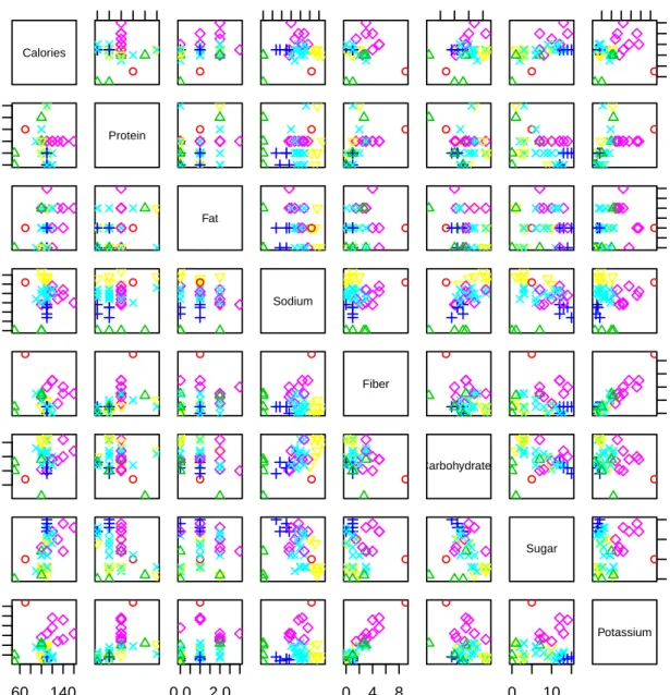
1.7 Example 1.2.1: Scatterplot matrix: The K-means cluster centers and

clus-ter assignments for the breakfast cereals data. . . 28

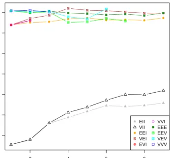
1.8 Example 1.2.1: BIC plot based on model-based clustering (mclust) for the

breakfast cereals data. . . 37

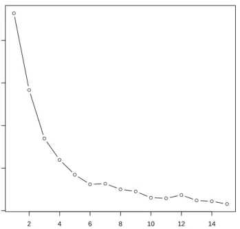
1.9 Example 1.2.1: Elbow plot for the breakfast cereals data. . . 41

1.10 Example 1.2.1: K-means partitions cascade comparison using a range of

values of K based on Calinski index for the breakfast cereals data. . . 43

1.11 Example 1.2.1: Gap plot for the breakfast cereals data. . . 45

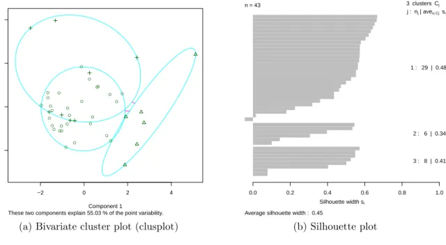
1.12 Example 1.2.1: Bivariate cluster plot (clusplot) and Silhouette plot based on the partitioning around medoids clustering (PAM) for the breakfast

cereals data. . . 46

2.1 Forward plot of minimum Mahalanobis distances from 100 randomly chosen

initial subsets for sample size n = 100 from bivariate mixture (a) normal,

(b) Laplace and (c) t distributions with uncorrelated variables. . . 60

2.2 Forward plot of minimum Mahalanobis distances from 100 randomly chosen

initial subsets for sample size n = 100 from bivariate mixture (a) normal,

2.3 Forward plot of minimum Mahalanobis distances from 100 randomly chosen

initial subsets for sample size n= 100 from trivariate mixture (a) normal,

(b) Laplace and (c) t distributions with uncorrelated variables. . . 64

2.4 Forward plot of minimum Mahalanobis distances from 100 randomly chosen

initial subsets for sample size n= 100 from trivariate mixture (a) normal,

(b) Laplace and (c) t distributions with correlated variables. . . 66

2.5 Forward plot of minimum Mahalanobis distances from 100 random starts

with 1%,50% and 99% envelopes for sample size n = 100 from bivariate

mixture normal distribution with uncorrelated variables. . . 68

2.6 Minimum Mahalanobis distances: 99% point for n = 200, 500, 700 and

1000 and d = 2, 5 and 10. Small d at the bottom of the plot. . . 69

2.7 Entry plot based on Mahalanobis distances fromm0 = 3with 100 randomly

chosen initial subsets for a mixture bivariate normal data set with 3 mixing

densities. . . 71

2.8 Forward plot based on Mahalanobis distances with 100 randomly chosen

initial subsets for a mixture bivariate normal data set with 3 mixing densities. 72

3.1 Forward plot of minimum spatial ranks from 100 randomly chosen initial

subsets for sample size n = 100 from bivariate mixture (a) normal, (b)

Laplace and (c) t distributions with uncorrelated variables. . . 81

3.2 Forward plot of minimum spatial ranks from 100 randomly chosen initial

subsets for sample size n = 100 from bivariate mixture (a) normal, (b)

Laplace and (c) t distributions with correlated variables. . . 83

3.3 Forward plot of minimum spatial ranks from 100 randomly chosen initial

subsets for sample size n = 100 from trivariate mixture (a) normal, (b)

Laplace and (c) t distributions with uncorrelated variables. . . 84

3.4 Forward plot of minimum spatial ranks from 100 randomly chosen initial

subsets for sample size n = 100 from trivariate mixture (a) normal, (b)

Laplace and (c) t distributions with correlated variables. . . 86

3.5 Forward plot of volume of central rank regions from 100 randomly chosen

initial subsets for sample size n = 100 from bivariate mixture (a) normal,

(b) Laplace and (c) t distributions with uncorrelated variables. . . 96

3.6 Forward plot of volume of central rank regions from 100 randomly chosen

initial subsets for sample size n = 100 from bivariate mixture (a) normal,

(b) Laplace and (c) t distributions with correlated variables. . . 97

3.7 Forward plot of volume of central rank regions from 100 randomly chosen

initial subsets for sample size n= 100 from trivariate mixture (a) normal,

(b) Laplace and (c) t distributions with uncorrelated variables. . . 98

3.8 Forward plot of volume of central rank regions from 100 randomly chosen

initial subsets for sample size n= 100 from trivariate mixture (a) normal,

3.9 Forward plot based on (a) spatial ranks and (b) volume of central rank regions, from 100 randomly chosen initial subsets for a mixture bivariate normal data set with 3 mixing densities. . . 101 3.10 Forward plot of volume of central rank regions from 100 random starts

with1%and 99%envelopes for sample sizen = 100from bivariate mixture

normal distribution with uncorrelated variables. . . 103

3.11 Entry plot based on spatial ranks from m0 = 3with 100 randomly chosen

initial subsets for a mixture bivariate normal data set with 3 mixing densities.104 3.12 Financial data: scatter-plot matrix. . . 105 3.13 Financial data: 3D scatter-plot. . . 106 3.14 Financial data: forward plot of minimum Mahalanobis distances among

units not in the subset from 100 random starts. Two clusters are evident

aroundm = 50. . . 107

3.15 Financial data: forward plot of volume of central rank regions among units

not in the subset from 100 random starts with1%and99%envelopes. Two

clusters are evident at m= 44 and 56. . . 108

3.16 Financial data: Cluster 1: left panel, scatterplot y1 vs y2, red points are

the units in cluster 1, and green points are unassigned units; right panel, forward plot of volume functional of central rank regions at the first peak

m= 56. . . 109

3.17 Financial data: Cluster 1: left panel, scatterplot y1 vs y2; right panel,

forward plot of volume of central rank regions atm = 102. . . 111

3.18 Financial data: Cluster 2: left panel, scatterplot y1 vs y2, red points are

the units in cluster 2, and green points are unassigned units; right panel, forward plot of volume functional of central rank regions at the first peak

m= 44. . . 113

3.19 Financial data: Cluster 2: left panel, scatterplot y1 vs y2; right panel,

forward plot of volume functional of central rank regions at m= 102. . . . 114

3.20 Financial data: (a) CH index suggestsK = 2, (b) K-means with 2 clusters,

and (c) BIC plot suggesting 6 clusters with best BIC values for EEE model. 117 3.21 Old faithful data: Scatter-plot . . . 118 3.22 Old faithful data: forward plot of volume of central rank regions among

units not in the subset from 100 random starts with1%and99%envelopes.

Two clusters are evident at m= 105 and 179. . . 119

3.23 Old faithful data: (a) CH index suggests K = 10, (b) K-means with 10

clusters, and (c) BIC plot suggesting 3 clusters with best BIC values for EEE model. . . 120

3.24 Iris data: Scatter-plot matrix . . . 121

3.25 Iris data: forward plot of volume of central rank regions among units not

in the subset from 100 random starts with 1% and 99% envelopes. Two

clusters are evident at m= 50 and 100. . . 122

3.26 Iris data: (a) CH index suggestsK = 3, (b) K-means with 3 clusters, and

4.1 Simulated data example: Contour plots of (a) Euclidean distances, (b) Mahalanobis distances, (c) spatial ranks, and (d) spatial depth based on 1000 random observations from bivariate mixture normal distribution with two groups. . . 132

4.2 Contour plots of the weighted spatial rank function (4.3.1) using: (a)

Gaussian, (b) Laplacian, (c) logistic, (d) triangular, (e) uniform, and (f) Epanechnikov kernel weights based on 1000 random observations from bi-variate mixture normal distribution with 2 groups. . . 134

4.3 Contour plots of the weighted spatial rank function (4.3.1) using generalized

Mallow at (a) r = 1, (b) r = 3, (c) r = 5 and (d) Naranjo weights based

on 1000 random observations from bivariate mixture normal distribution with 2 groups. . . 137

4.4 Contour plots of the weighted spatial rank function (4.3.2) using: (a)

Gaussian, (b) Laplacian, (c) logistic, (d) triangular, (e) uniform, and (f) Epanechnikov kernel weights based on 1000 random observations from bi-variate mixture normal distribution with 2 groups. . . 139

4.5 Contour plots of the weighted spatial rank function (4.3.2) using generalized

Mallow at (a) r = 1, (b) r = 3, (c) r = 5 and (d) Naranjo weights based

on 1000 random observations from bivariate mixture normal distribution with 2 groups. . . 142

4.6 The steps of the weighted spatial ranks based clustering algorithm . . . 148

4.7 Simulated data 1: (a) scatterplot matrix of the PCA components, (b) the

total variance explained by each component, (c) the weighted spatial ranks contour, (d) the contour at level 0.005 and confirmatory plots based on weighted ranks classifier for (e) the first 2 components and (f) the original data. . . 150

4.8 Simulated data 2: (a) scatterplot matrix of the PCA components, (b) the

total variance explained by each component, (c) the weighted spatial ranks contour, (d) the contour at level 0.001 and confirmatory plots based on weighted ranks classifier for (e) the first 2 components and (f) the original data. . . 153

4.9 Iris data: (a) scatterplot matrix of the PCA components, (b) the total

vari-ance explained by each component, (c) the weighted spatial ranks contour, (d) the contour at level 0.07 and confirmatory plots based on weighted

ranks classifier for (e) the first 2 components and (f) the original data. . . 156

4.10 Financial data: (a) scatterplot matrix of the PCA components, (b) the total variance explained by each component, (c) the weighted spatial ranks contour, (d) the contour at level 0.0006 and confirmatory plots based on weighted ranks classifier for (e) the first 2 components and (f) the original data. . . 158 4.11 Old faithful data: (a) scatterplot of the faithful data, (b) the weighted

spatial ranks contour, (c) the contour at level 0.005 and (d) confirmatory plots based on weighted ranks classifier for original data. . . 160

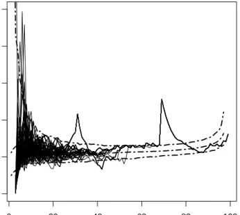
5.1 Gun-point and growth data curves with two groups for both datasets. Black curves are the curves in cluster 1, and red curves are the curves in cluster 2.169

5.2 CH index scores and K-means clustering for the discretized gun-point and

growth datasets. CH index suggests 2 and 7 clusters for gun point and growth data respectively. . . 172

5.3 K-centroids clustering (kcca) for the discretized (a) gun-point data and (b)

growth data. . . 173

5.4 Linkage based methods for the discretized gun-point and growth datasets. . 174

5.5 BIC and ICL plots based on Gaussian Mixture Models (GMM) for the

discretized gun-point and growth datasets. One cluster is evident for both data. . . 177

5.6 Cattell’s scree-test and BIC criterion based on High Dimensional Data

Clustering (HDDC) for the discretized gun point and growth datasets sug-gest the intrinsic dimensions. . . 178

5.7 BIC plot based on the mixtures of probabilistic principle component

anal-ysers (MixtPPCA) for the discretized: (a) gun-point data suggests 4 PCs and 4 groups, and (b) growth data suggests 4 PCs and 2 groups. . . 179

5.8 Bivariate cluster plot (clusplot) and silhouette plot based on the

partition-ing around medoids clusterpartition-ing (PAM) for the discretized: (a) gun-point data suggest 3 groups, and (b) growth data suggest 2 groups. . . 180

5.9 Convex clustering (cclust) based on the hard competitive learning method

for the discretized: (a) gun point data and (b) growth data. . . 181

5.10 Banner and dendrogram plots of a divisive hierarchical clustering based on the DIvisive ANAlysis algorithm (DIANA) for the discretized gun-point and growth datasets. . . 183 5.11 Bivariate cluster plot (clusplot) and silhouette plot based on the Clustering

Large Applications (CLARA) algorithm for the discretized: (a) gun-point

data and (b) growth data. Two groups are evident for both data. . . 184

5.12 CH index scores and K-means clustering for the FPCA scores of gun-point and growth datasets. CH index suggests 9 and 5 clusters for gun point and growth data respectively. . . 189 5.13 K-centroids clustering (kcca) for the FPCA scores of (a) gun-point data

and (b) growth data. . . 190 5.14 Linkage based methods for the FPCA scores of gun-point and growth

datasets. . . 191 5.15 BIC and classification uncertainty plots based on Gaussian Mixture Models

(GMM) for the FPCA scores of gun-point and growth datasets. Nine and two clusters are evident for gun-point and growth data respectively. . . 193 5.16 Cattell’s scree-test and BIC criterion based on High Dimensional Data

Clustering (HDDC) for the FPCA scores of gun point and growth datasets suggest the intrinsic dimensions. . . 194

5.17 BIC plot based on the mixtures of probabilistic principle component anal-ysers (MixtPPCA) for the FPCA scores of gun-point and growth datasets suggests 1 PC and 1 group for both data. . . 195 5.18 Bivariate cluster plot (clusplot) and silhouette plot based on the

partition-ing around medoids clusterpartition-ing (PAM) for the FPCA scores of: (a) gun-point data suggest 4 groups, and (b) growth data suggest 5 groups. . . 197 5.19 Convex clustering (cclust) based on the hard competitive learning method

for the FPCA scores of: (a) gun point data and (b) growth data. . . 198 5.20 Banner and dendrogram plots of a divisive hierarchical clustering based on

the DIvisive ANAlysis algorithm (DIANA) for the FPCA scores of gun-point and growth datasets. . . 199 5.21 Bivariate cluster plot (clusplot) and silhouette plot based on the Clustering

Large Applications (CLARA) algorithm for the FPCA scores of: (a) gun-point data suggest 2 groups and (b) growth data suggest 4 groups. . . 200 5.22 CH index scores and K-means clustering for the spline coefficients of

gun-point and growth datasets. CH index suggests 2 clusters for both data. . . 203 5.23 K-centroids clustering (kcca) for the spline coefficients of (a) gun-point data

and (b) growth data. . . 204 5.24 Linkage based methods for the spline coefficients of gun-point and growth

datasets. . . 205 5.25 BIC and ICL plots based on Gaussian Mixture Models (GMM) for the

spline coefficients of gun-point and growth datasets. Seven and three clus-ters are evident for gun-point and growth data respectively. . . 207 5.26 Cattell’s scree-test and BIC criterion based on High Dimensional Data

Clustering (HDDC) for the spline coefficients of gun point and growth datasets suggest the intrinsic dimensions. . . 209 5.27 BIC plot based on the mixtures of probabilistic principle component

analy-sers (MixtPPCA) for the spline coefficients of: (a) gun-point data suggests 4 PCs and 4 groups, and (b) growth data suggests 4 PCs and 2 groups. . . 210 5.28 Bivariate cluster plot (clusplot) and silhouette plot based on the

parti-tioning around medoids clustering (PAM) for the spline coefficients of: (a) gun-point data suggest 3 groups, and (b) growth data suggest 2 groups. . . 211 5.29 Convex clustering (cclust) based on the hard competitive learning method

for the spline coefficients of: (a) gun point data and (b) growth data. . . . 212 5.30 Banner and dendrogram plots of a divisive hierarchical clustering based

on the DIvisive ANAlysis algorithm (DIANA) for the spline coefficients of gun-point and growth datasets. . . 213 5.31 Bivariate cluster plot (clusplot) and silhouette plot based on the Clustering

Large Applications (CLARA) algorithm for the spline coefficients of gun-point data suggest 2 groups and growth data suggest 6 groups. . . 214

5.32 Clustering of gun-point and growth datasets using fclust method. . . 216

5.33 Clustering of gun-point and growth datasets using the wavelets-based method (curvclust algorithm) . . . 217

5.34 FunHDDC clustering: Plots of functional data curves and functional data means based on FunHDDC coefficients for gun-point and growth datasets . 219 5.35 Clustering of gun point and growth datasets using funclust algorithm . . . 220 5.36 K-means clustering for functional data (kmeans.fd algorithm): plot of the

curves and the updated centers based on kmeans.fd for the gun-point and growth datasets. . . 221 5.37 Clustering of the gun-point and growth datasets using K-means based on

the distance d0 (Kmeans-d0). . . 224

5.38 Clustering of the gun-point and growth datasets using K-means based on

the distance d1 (Kmeans-d1). . . 224

5.39 Simulated data, Model 1: (a) the observed curves with two groups, (b) the mean function, (c) the forward plot based on FSR and (d) the entry plot based on FSR. . . 235 5.40 Simulated data, Model 2: (a) the observed curves with two groups, (b) the

mean function, (c) the forward plot based on FSR and (d) the entry plot based on FSR. . . 237 5.41 Simulated data, Model 3: (a) the observed curves with three groups, (b)

the mean function, (c) the forward plot based on FSR and (d) the entry plot based on FSR. . . 238 5.42 Gun-point data: Forward plot based on the functional spatial ranks. Two

clusters are evident around subsets with sizes 100. . . 239 5.43 Growth data: Forward plot based on the functional spatial ranks. Two

clusters are evident around subsets with sizes 39 and 54. . . 240 5.44 ECG data: panel (a) is the observed curves with two groups and panel (b)

is the forward plot based on the functional spatial ranks. Two clusters are

evident around subsets with sizes 67 and 133. . . 241

5.45 Simulated data, Model 1: (a) the observed curves with two groups, (b) plot of the functional PCA with the total variance explained by each harmonic, (c) the WFSR contours, (d) the contour at level 0.002, and confirmatory plots based on WFSRC for (e) the first 2 components and (f) the observed curves. . . 248 5.46 Simulated data, Model 2: (a) the observed curves with two groups, (b) plot

of the functional PCA with the total variance explained by each harmonic, (c) the WFSR contours, (d) the contour at level 0.005, and confirmatory plots based on WFSRC for (e) the first 2 components and (f) the observed curves. . . 250 5.47 Simulated data, Model 3: (a) the observed curves with three groups, (b)

plot of the functional PCA with the total variance explained by each har-monic, (c) the WFSR contours, (d) the contour at level 0.01, and confir-matory plots based on WFSRC for (e) the first 2 components and (f) the observed curves. . . 253

5.48 Gun-point data: (a) plot of fd curves after smoothing, (b) plot of the functional PCA with the total variance explained by each harmonic, (c) the WFSR contours, (d) the contour at level 0.02, and confirmatory plots based on WFSRC for (e) the first 2 components and (f) the observed curves.255 5.49 Growth data: (a) plot of fd curves after smoothing, (b) plot of the

func-tional PCA with the total variance explained by each harmonic, (c) the WFSR contours, (d) the contour at level 0.011, and confirmatory plots based on WFSRC for (e) the first 2 components and (f) the observed curves.257

List of Tables

1.1 Counts of binary outcomes for two items. . . 7

1.2 Common similarity measures for the binary data based on the frequencies. 8

1.3 Example 1.2.1: CH index for the breakfast cereals data based on the

K-means clustering method. . . 26

1.4 Example 1.2.1: The K-means cluster centers for the breakfast cereals data. 27

3.1 Financial data: The volume of central rank regions for each subset (m) for

Cluster 1 . . . 109

3.2 Financial data: The assigned units in the first cluster by using forward

search based on volume of central rank regions (55 units). . . 112

3.3 Financial data: The volume of central rank regions for each subset (m) for

Cluster 2 . . . 114

3.4 Financial data: The assigned units in the second cluster by using forward

search based on volume of central rank regions (43 units). . . 115

4.1 The probabilities of misclassification error based on the different clustering

methods for faithful, financial and iris datasets. . . 163

5.1 The probabilities of misclassification error based on the different functional

data clustering approaches for gun-point dataset. . . 260

5.2 The probabilities of misclassification error based on the different functional

Chapter 1

Introduction

1.1

Introduction

Recently, cluster analysis has become one of the most important statistical tools to study and clarify many scientific disciplines that require to cluster data in the aim to understand and interpret the studied phenomenon. It is a helpful exploratory tool for analysis of the low and high dimensional multivariate data and functional data as well. A particular attention is paid to the cluster analysis for the higher dimensional data. There have been many clustering methods, techniques and algorithms scattered in publications in very di-versified areas such as pattern recognition, artificial intelligence, information technology, image processing, biology, psychology, market research, astronomy, psychiatry, weather classification, archaeology, bioinformatics and genetics (Gan et al., 2007; Everitt et al., 2011). However, the problem of determination the best number of clusters has been con-sidered a kind of limitation in the most previous studies. Moreover, choosing a suitable clustering technique is another serious issue in cluster analysis. We postpone the discus-sion on the first problem to Section 1.6, where we present some of the common ways that try to address this problem of estimating the number of clusters, while we address the discussion on the second point to the next two Sections.

Examples of the first literature that discussed the clustering analysis have been given by Hartigan (1975), where the word clustering was known at this time as the numerical taxonomy. Sokal and Sneath (1963) has considered the first and most important book in numerical taxonomy. Some methods of measuring similarity are proposed in it, with

particular attention given to category data. Clustering analysis is also known as

Q-analysis, clumping, unsupervised learning, and typology. Many definitions for cluster analysis have been used in the literature. A simple one that has been considered by Hartigan (1975) is: “clustering is the grouping of similar objects”. Jain and Dubes (1988) have defined the cluster analysis as “the formal study of algorithms and methods for grouping or classifying objects”, while Kaufman and Rousseeuw (2005) defined it as “the art of finding groups in data”. In pattern recognition and neural network studies, cluster analysis is known as unsupervised learning (training patterns with unknown category labels), and it is called segmentation analysis especially in the market studies.

It can be clearly seen that, all the previous definitions agree on an important point that the cluster analysis aims to group and partition a given set of data or objects into clusters, subsets, or groups, we need to know any properties should to be in this partitioning. The first property or assumption is the homogeneity within the clusters, i.e. points that belong to the same cluster should be as similar as possible. The second one is the heterogeneity between clusters, i.e. points that belong to different clusters should be as different as possible (Hoppner et al., 1999).

In order to illustrate the importance of cluster analysis, we provide some common examples that are usually used in the literature. The first example is the taxonomy of animals and plants. Taxonomy is the science of describing, naming, and classifying organ-isms which are described by their structure, appearance and hypothesized evolutionary relationships. The main interest of this science is that we need to cluster each animal, plant and species in the best way, which implies the homogeneity within the clusters and

the heterogeneity between clusters.

The same methodology can be considered for the phylogenetic tree of life, where there are three domains of life bacteria, archaea, eukarya and each of them consists of some components. For instance, the bacteria consist of 9 components while the animals and plants belong to the eukarya which contains 10 components as shown in Figure 1.1 (c). This tree gives a good example for the importance of the cluster analysis in our life, since it has provided physical significance in the evolutionary theories of Darwin. Figure 1.1 shows some examples of the taxonomy of animals and plants, where plots (a), (b), (c) and (d) give the evolutionary tree, classification of plant tissues, phylogenetic tree of life and general tree of life respectively.

A third example is the handwriting recognition. Recently, the handwriting recogni-tion has become one of the important topics after the computerized informarecogni-tion revolurecogni-tion has appeared. Many publications have been introduced and discussed some graphical ap-proaches and statistical clustering algorithms that can be used to detect the handwriting numbers. Handwriting recognition concerns with the ability and performance of a com-puter to reed and interpret some handwritten inputs. These inputs may come from either paper documents or touchscreens. Cluster analysis and its novel algorithms that are intro-duced continuously, play an important role in this topic. Figure 1.2 shows some examples of the handwriting recognition, where plots (a) and (b) give the hierarchical clustering of handwritten numbers of a particular writer and some different handwritten numbers respectively.

Many other examples that show the importance of the cluster analysis could be given in this context, for example, one of the common cluster analysis examples is measuring the similarities of 11 languages, which has been introduced by Johnson and Wichern (2007). In this example, the main interest is clustering the most like European languages that use the Roman alphabet based on the numeral of these 11 languages.

(a) Evolutionary tree (b) Plant tissue classification

(c) Phylogenetic tree of life (d) General tree of life

Figure 1.1: Examples of cluster analysis: The taxonomy of animals and plants (a) Evolu-tionary tree[64], (b) Classification of plant tissues[163], (c) Phylogenetic tree of life[162] and (d) General tree of life[75].

We cannot leave these examples of cluster analysis without mentioning the gene ex-pression data topic, since cluster analysis is one of the most frequently approaches that are used to analyze the gene expression data. A particular attention is paid to the cluster analysis for the gene expression data, which is helpful to understand the functions of genes whose information has not been previously available (Eisen et al., 1998). As an example, a biologist would like to find out the clusters from the DNA microarray data on gene expressions, and consequently detecting the classes or subclasses of diseases. Full details about the cluster analysis for gene expression data can be found in (Gan et al., 2007). A good collection of the cluster analysis examples are available in (Hartigan, 1975; Gan et al., 2007; Everitt et al., 2011).

(a) Hierarchical clustering of handwritten numbers of a par-ticular writer

(b) Different handwritten numbers

Figure 1.2: Examples of cluster analysis: The handwriting recognition (a) Hierarchical clustering of the 12 pen-strokes centroids of a particular writer[101], (b) Different hand-written numbers[53].

1.2

Hierarchical Clustering Methods

There are two major concerns in the existing literature regarding to the clustering tech-niques; hierarchical clustering techniques and non-hierarchical clustering techniques. How-ever, the graphical approaches have been considered a third concern in literature. In this Section, we will discuss the similarity measures, the distance measures, the hierarchical clustering techniques and the graphical approaches.

In order to measure the homogeneity within or between clusters, we need to use some similarity measures. The similarity and dissimilarity measures in many cases are based on some measures of distance that help us to use some techniques in order to group the observations into clusters. Logically, after we use one of these measures, we need to apply some approach which can be considered as the initial clustering indicator. The graphical approaches are very useful approaches that give us initial view about if the data may

it. Two common types of techniques, known as hierarchical clustering techniques and non-hierarchical clustering techniques are usually used as attempt to find all grouping possibilities.

In order to measure the similarity between groups or samples, a measure of similar-ity or dissimilarsimilar-ity has to be defined. According to the data types, similarsimilar-ity measures can be used to determine either the similarity between entities or groups. For instance, one can use the association coefficients as similarity measure if the variable is binary, or use Gower coefficient (Gower, 1971) if the data is multinomial or quantitative data. Alternatively, dissimilarity (distance) measures can be used to determine the distance degree between entities or groups. A similarity coefficient indicates the strength of the relationship between two data points (Everitt, 1993). The various measures can be de-fined for several types of data such as: numerical, categorical, binary and mixed-typed data. Sneath and Sokal (1973), subdivided the similarity and dissimilarity coefficients into four groups; correlation coefficients, distance measures, association coefficients, and probabilistic similarity measures.

It is worth mentioning that there are two types of similarity or distance measures, the first is between entities (individuals) and the second is between groups. As we focus on measuring the similarity between entities, we give brief discussion about the similarity and dissimilarity measures between entities in Sections 1.2.1 and 1.2.2 respectively.

1.2.1

Similarity Measures

Similarity measures are used to describe how similar two data points (two clusters) are. There are many ways to measure the similarity or proximity between pairs of objects. One can consider the association coefficients as a similarity measures for the binary data, in order to cluster items, where each variable takes two cases in terms of counts of matches and mismatches (presence and absence) in each variable for two individuals. Suppose

that a represents the frequency of1−1 matches,b is the frequency of1−0matches, cis

the frequency of 0−1matches, and dis the frequency of 0−0matches, then we can put

the frequencies of the matches and mismatches for item i and item k in the form of the

contingency table 1.1:

Table 1.1: Counts of binary outcomes for two items. Item k

Outcome 1 0 Total

Item i 1 a b a+b

0 c d c+d

Total a+c b+d p=a+b+c+d

There are many association coefficients that depend on the 2 by 2 association table like matching coefficient, Jaccard (1908) coefficient, Rogers and Tanimoto (1960) coefficient, Sneath and Sokal (1973) coefficient, and Gower and Legendre (1986) coefficient. More extensive coefficients can be found in Gower and Legendre (1986). Table 1.2 shows the common similarity measures for the binary data based on the frequencies in Table 1.1.

One of the important similarity measures that can be used to cluster variables is the correlation coefficient, which suggested by Karl Pearson (Pearson, 1920). Suppose that our variables are binary which can arranged in the contingency table 1.1, so we can get the usual product moment correlation coefficient, which is considered a common measure of the similarity between two binary variables and equivalent to the chi-square statistic for testing the independence of two categorical variables, as following:

r = ad−bc

[(a+b)(c+d)(a+c)(b+d)]1/2. (1.2.1)

Jukes and Cantor (1969), Tajima (1993) and Dyen et al. (1992) suggested some

similarity measures for categorical data with more than two levels, while Gower (1971) proposed an important similarity measure that can apply for binary, multinomial, metric

Table 1.2: Common similarity measures for the binary data based on the frequencies.

Measure Coefficient Name

a+d

a+b+c+d Matching coefficient: Sokal and Michener

a

a+b+c Jaccard coefficient

a+d

a+2(b+c)+d Rogers and Tanimoto coefficient

a

a+2(b+c) Sneath and Sokal coefficient

a+d

a+1/2(b+c)+d Gower and Legendre coefficient

a

a+1/2(b+c) Gower and Legendre coefficient

2a

2a+b+c Czekanowski, Dice and Sorensen coefficient

a

a+b+c+d Russell and Rao coefficient

a

b+c Ratio of matches to mismatches coefficient

(quantitative), and mixed data. Suppose that SMik is the mean of similarity coefficient

between the two points k, i ; xij is the i−th observation for the variable j; and p is the

number of variables, then Gower’s coefficient for the mixed data takes the form:

SMik = Pp j=1SMikj Pp j=1Wikj ; i6=k = 1, ..., n (1.2.2)

where Wikj is a weight that takes two values, 1 when both entities i, k have the same

property that we are interested in, and 0 otherwise; andSMikj is the similarity coefficient

between the two entitiesiand kbased on the variable j, which can be calculated in many

1.2.2

Distance Measures

On the contrary of the similarity measures, dissimilarity (distance) measures determine

the degree of distance between two entities, items or groups. Four standard criteria

(mathematical properties), that can be used to judge whether a similarity measure is a true metric or not, are mentioned in Aldenderfer and Blashfield (1984), however not all the distance measures mentioned below are metrics.

The most popular distance measure, which is usually used for the numerical data, is the Euclidean distance (squared Euclidean distance, when the value of distance is squared).

This distance is also known as thel2 norm. Letdik be the distance between the two points

k and i; xij is the i−th observation for the variable j; and p is the number of variables,

then the Euclidean distance can be written as:

dik = ( _p X j=1 (xij −xkj)2 )1/2 . (1.2.3)

However, it is well known that the Euclidean distance is affected by changes in the units of measurement, for example we would get two different values for the Euclidean distance between the weight and height if we considered the unit of measurement for the weight variable is kilograms instead of lbs. To address this problem, we need to standardize the variables by dividing by the standard deviation of each variable, such that:

dik = ( _p X j=1 (xij −xkj)2 σ2 j )1/2 . (1.2.4)

this standardized form is not affected by the changes in the units of measurement. Another

way to standardize the variables is based on the rangeRjinstead of the standard deviation.

It is known as the maximum distance, which is defined to be the maximum value of the distances of the attributes, such that:

Rj = max

i,k |xij −xkj|. (1.2.5)

Another well-known metric, which is used for the numerical data, is the city block or

Manhattan distance (l1 norm). The Manhattan distance was used in a cluster analysis

context by Carmichael and Sneath (1969). It is usually used when the units of measure-ment are same for all the variables, and it takes the form:

dik = p

X

j=1

Wj|xij −xkj|. (1.2.6)

It is worth mentioning in this context that, the Euclidean metric, Manhattan metric

and maximum distance in (1.2.5) are special cases of the general Minkowski distance (lr)

atr= 2,1and∞respectively, where r is called the order of the Minkowski distance, and

they satisfy the mathematical requirements of a distance function. The general form of Minkowski distance is:

dik = ( _p X j=1 Wj|xij −xkj|r )1/r . (1.2.7)

In literature Mahalanobis distance, also called generalized distance (Mahalanobis, 1936), has been considered as a very important metric that can be used for the nu-merical data. It takes the correlations among variables in the account by the inclusion of

the variance-covariance matrix Σ, therefore, this distance applies a weight scheme to the

data. The second feature is that Mahalanobis distance is invariant under all nonsingular

transformations. When the correlation between variables is zero, Σ is the identity

ma-trix; the squared Mahalanobis distance is same as the squared Euclidean distance. The

Mahalanobis distance between two points X_i = (Xi1, ..., Xid)T and Xk = (Xk1, ..., Xkd)T

dik=

p

(Xi −Xk)TΣ−1(Xi−Xk). (1.2.8)

A generalized Mahalanobis distance has been introduced by Morrison (1967), where the weight of each variable has been included in the measure by adding a diagonal matrix

containing the p weights. At the same time, Gower (1967) suggested another distance

measure for the numerical data which can be calculated by using the form:

dik =−log10 1− 1 p p X j=1 |xij −xkj| βj −αj ! . (1.2.9)

where αj = mini6=k(xij −xkj) and βj = maxi6=k(xij −xkj). Many other non-metric

dis-tance measures for the numerical data that do not meet the metric conditions have been introduced over the literature. For instance, Sokal and Sneath (1963) proposed a distance function in order to measure the distance between two entities, such that:

dik = v u u t 1 p p X j=1 (xij −xkj) (xij +xkj) 2 . (1.2.10)

Canberra distance measure, introduced by Lance and Williams (1967), is often re-garded as a generalization of the dissimilarity measure for binary data. They proposed the following two distance measures:

d(L)_ik = Pp j=1|xij −xkj| Pp j=1|xij +xkj| , d(W_ik )= Pp j=1|xij −xkj| Pp j=1|xij|+|xkj| . (1.2.11)

Although all the above distance measures are used for the numerical data, there are many other distance measures that can be used for the categorical, binary and mixed data. For example, the simple matching dissimilarity measure and Harrison (1968) measure are usually used for the categorical data. Moreover, some studies suggested that we can use the relationship between the similarity and dissimilarity measures in order to get a distance

measure for the categorical data. So, one can use the transformation dik = 1−SMik ,

if the data is binary, or Gower (1966,1967) transformation, dik =

p

2 (1−SMik) , if the

data is mixed data.

1.2.3

Agglomerative Hierarchical Methods

Two common types of methods, known as agglomerative hierarchical methods and divisive hierarchical methods, are usually used under the hierarchical clustering techniques. For the first type of methods, agglomerative hierarchical methods, they depend on the merging process so that we start with number of groups equals to the number of elements, in other words each element is in a cluster of its own. The most similar elements are first grouped, and then these groups are also merged, until all elements end up being in the same cluster. The result of the clustering can be displayed as a dendrogram, which illustrates the merger that have been made.

Linkage-Based Methods

In order to use one of the agglomerative hierarchical methods, we have to start by calcu-lating the similarity or dissimilarity matrix between entities, and finish with the dendro-gram. The most common and important agglomerative hierarchical methods are; single linkage, complete linkage, average linkage, coordinate centroid clustering, median clus-tering method, Ward’s hierarchical clusclus-tering method and Lance and Williams flexible method. The only difference between the various agglomerative hierarchical methods, is that how can we calculate the similarity or distance measures between entities or sub-groups. For instance, in the single linkage, complete linkage, and average linkage methods we start by searching about the most two similar elements in the distance (similarity) matrix, then we merge them to form the first cluster. The next step is calculating the distances between this cluster and the remaining elements by using specific distance func-tion. After that, we continue in choosing the most two similar elements (clusters) in the

distance (similarity) matrix until all elements end up being in the same cluster. It is worth mentioning that, each of these three methods has its own distance function. The single linkage method has been considered one of the oldest methods of cluster analysis; it was suggested independently by Florek et al. (1951), McQuitty (1957) and Sneath (1957). Sibson (1973) proposed an important optimality efficient algorithm (SLINK) for the single linkage method, which can be applied on an unprecedented scale. Recently, many publications have developed this method. A useful overview is given in Muja and Lowe (2009), where they suggested an automatic algorithm to get fast approximate of the nearest neighbors and a system which takes any given dataset and desired degree of precision and use these to automatically determine the best algorithm and parameter values. On the other hand, the complete linkage method has been developed by Lance and Williams (1967) and Johnson (1967). Along the line of Sibson (1973), Defays (1977) introduced an efficient algorithm for the complete linkage method which is based like the (SLINK) algorithm and offers economy in computation. Following, we give brief discus-sion regarding to the three linkage-based methods, (single linkage, complete linkage, and average linkage methods).

We can conclude the main steps of the agglomerative hierarchical clustering algorithm as the following:

1. We start with number of groups equals to the number of elements, where each

element is in a cluster of its own. Suppose we have n items, so we get firstly

n×n distance (similarity) matrix by using any one of the measures that we have

mentioned above.

2. In this step, we start by searching about the most two similar elements in the

distance (similarity) matrix. Suppose that the most similar items (clusters) are i

3. An update in the distance matrix should be done by omitting the rows and columns

corresponding to items (clusters) i and k, and then we should add a new row and

column giving the distances between cluster (i, k) and the other items (clusters)

by using some distance function, where each method of them has its own distance function as we show below.

4. Continue in choosing the most two similar elements (clusters) in the distance (sim-ilarity) matrix and update it until all elements end up being in the same cluster.

Single Linkage Method

The single linkage method, which is also known as nearest neighbour clustering, depends

on the nearest-neighbour rule. In this method, the distance between specific cluster (t)

and another cluster (ik) that consists of the two entities i and k is calculated by using

the distance function:

dt(ik)= min

i6=k (dit, dkt), (1.2.12)

or

SMt(ik) = max

i6=k (SMit, SMkt), (1.2.13)

if we use a similarity matrix instead of dissimilarity matrix.

Complete Linkage Method

On the other hand, the complete linkage method, which is also known as farthest neigh-bour clustering, depends on the furthest-neighneigh-bour rule. In this method, the distance

between specific group (t) and another group (ik) is calculated by using the distance

function:

dt(ik) = max

or

SMt(ik) = min

i6=k (SMit, SMkt), (1.2.15)

if we use a similarity matrix.

Average Linkage Method

In the third agglomerative hierarchical method, average linkage, which is also known as unweighted pair group method with arithmetic mean (UPGMA), the distance between two clusters can be considered as the average distance between all pairs of items where one member of a pair belongs to each cluster (Johnson and Wichern, 2007). Suppose that

n(ik) andntare the number of items in clusters(ik)andt, respectively, then the distance,

duv, between object u in the clustert and object v in the cluster (ik) is obtained by:

dt(ik) = P u P vduv n(ik).nt , (1.2.16) or SMt(ik) = P u P vSMuv n(ik).nt , (1.2.17)

if we use a similarity matrix.

Example 1.2.1 Breakfast Cereals Data

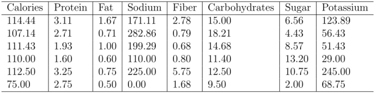
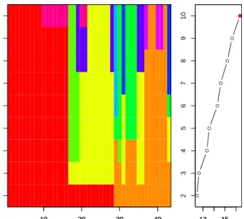
In this example, we consider the data on brands of breakfast cereals [Source: Data courtesy of Chad Dacus, Table 11.9 of Johnson and Wichern (2007)], which contains 43 types of breakfast cereals produced by three different American companies (General Mills (G), Kellogg’s (K), and Quaker (Q)). It also contains eight variables, where eight numerical nutritional characteristics have been measured for each cereal. The variables are: Calories, Protein, Fat, Sodium, Fiber, Carbohydrates, Sugar, and Potassium. Also, the name of each cereal and the company that produced the cereal have been given.

Our target is clustering these 43 types of breakfast cereals based on the above 8 vari-ables, by using the linkage-based methods (single, complete and average linkage meth-ods). As we mentioned in the agglomerative hierarchical clustering algorithm, we start with number of groups equals to the number of breakfast cereals types (43), and we start clustering by merging the two cereals that have smallest nonzero distance in the distance matrix until all the cereals end up being in the same cluster. Figures 1.3, 1.4 and 1.5 show the single, complete and average linkage dendrograms for the distances between the 43 types of breakfast cereals respectively, where they illustrate the grouping and the partitions produced at each stage, for each method.

As we can see in Figure 1.3, the single linkage dendrogram does not give a clear clustering and it is very difficult visually to determine the number of clusters from the dendrogram. This is due to the distances between observations are not big enough to distinguish the separation between groups. For example, if we cut the tree at the height

h = 100, then we get two clusters, one of them with only one cereals brand (AllBran) and the second cluster with the remaining 42 cereals brands. However, cutting the tree

at h = 85 gives 3 clusters, which in fact means for each point xij, every other point xkj

in its cluster satisfies dik 6 85, where dik is the Euclidean distances defined in (1.2.3).

Compared to Figure 1.4, it can be clearly seen that the complete linkage dendrogram shows clearer clustering structure, where it is obviously gives an evidence about the existence of three clusters. The distances in this dendrogram are much wider, and that makes it easy visually to distinguish the number of clusters. For instance, cutting the complete

linkage tree ath= 250 gives 3 clusters, which means for each pointxij, every other point

xkj in its cluster satisfies dik 6 250. For the average linkage method, we can see from

Figure 1.5 that the dendrogram does not give reasonable result as the distances are not wide enough comparing to them in the complete linkage method. Like the single linkage dendrogram, the average one has assigned only one cereals brand (AllBran) in one cluster.

So, we can conclude that the complete linkage method outperforms both of the single and average linkage methods in this data. From this example, we can see that determining the cutting point in the linkage based methods is questionable, and may require some different methods to decide the right number of clusters.

Other Agglomerative Hierarchical Methods

The coordinate centroid clustering method, which is also known as unweighted pair-group method using the centroid approach (UPGMC), has been suggested by Sokal and Michener (1958), and then developed by King (1967) in order to cluster the variables. This method tries to merge each two subgroups to be fused together depending on the distance between their coordinate centroids. It starts also by searching about the most two similar elements in the distance matrix, then merging them to form the first cluster and calculate its corresponding centroid in order to adjust the distance matrix. We continue in choosing the most two similar elements (subgroups) in the distance matrix until all elements end up being in the same cluster like the linkage-based methods.

A disadvantage of this method is that, it is affected by the group size when one of the two subgroups to be fused has very different size than the other such that the centroid of two merged groups will be very close to that of the larger group and may remain within that group, and consequently the smaller group will lose its properties. For that reason, Gower (1967) has suggested the median clustering method, which assumes the equality of the size of each group to be fused.

Ward (1963) has introduced another hierarchical clustering procedure, which is de-pending on the error sum of squares (ESS) criterion. He pointed out that with each merging occur, there will be some loss of information, which can be measured by calcu-lating the error sum of squares. According to Ward’s method, one can consider that a merged group is acceptable if the increase in the total within-cluster error sum of squares

AllBran MueslixCrisp

yBlend ainAlmondRaisin NutriGr

T rix AppleJacks FrootLoops CornP ops Smacks RaisinNutBran CracklinOatBr an Cheerios OatmealRaisinCrisp HoneyNutCheer ios MultiGrainCheer

ios ain T otalWholeGr

Cheaties Product19 Kix GoldenGrahams CornFlak es RiceKrispies WheatiesHoneyGold JustRightCr unchyNuggets CocoaPuffs LuckyCharms ACCheer ios CountChocula NutNHoneyCr

unch nFlakes T otalCor

FrostedFlakes SpecialK Crispix CapNCrunch HoneyGr ahamOhs NutriGr ainWheat Life FruitfulBr an T otalRaisinBr an RaisinBran FrostedMiniWheats QuakerOatmeal PuffedRice PuffedWheat 0 20 60 100

Cluster Dendr

ogram

T rix AppleJacks FrootLoops CornP ops Smacks FrostedMiniWheats QuakerOatmeal PuffedRice PuffedWheat Cheerios HoneyNutCheer ios Product19 Kix GoldenGrahams CornFlak es RiceKrispies WheatiesHoneyGold ACCheer ios CountChocula JustRightCr unchyNuggets CocoaPuffs LuckyCharms NutNHoneyCr

unch nFlakes T otalCor

FrostedFlakes SpecialK Crispix CapNCrunch HoneyGr ahamOhs OatmealRaisinCrisp NutriGr ainWheat

Life ainAlmondRaisin NutriGr

MultiGrainCheer

ios ain T otalWholeGr

Cheaties AllBran MueslixCrisp yBlend RaisinNutBran CracklinOatBr an FruitfulBr an T otalRaisinBr an RaisinBran 0 100 200 300 400

Cluster Dendr

ogram

AllBran FrostedMiniWheats QuakerOatmeal PuffedRice PuffedWheat MueslixCrisp yBlend RaisinNutBran CracklinOatBr an FruitfulBr an T otalRaisinBr an RaisinBran T rix AppleJacks FrootLoops CornP ops Smacks Product19 Kix GoldenGrahams CornFlak es RiceKrispies Cheerios HoneyNutCheer ios WheatiesHoneyGold JustRightCr unchyNuggets CocoaPuffs LuckyCharms ACCheer ios CountChocula NutNHoneyCr

unch nFlakes T otalCor

FrostedFlakes SpecialK

Crispix CapNCrunch

HoneyGr

ahamOhs ainAlmondRaisin NutriGr

MultiGrainCheer

ios ain T otalWholeGr

Cheaties OatmealRaisinCrisp NutriGr ainWheat Life 0 50 150 250

Cluster Dendr

ogram

this method as the minimum variance method. Lance and Williams (1967) have

suggested a recurrence formula that gives the distance between two clusters t and (i, k),

the formula is given by:

dt(i,k) =αidti+αkdtk+βdik+γ|dti−dtk|,

where dik is the distance between groups i and k while α, β and γ are parameters whose

values are different for different methods above. It is worth mentioning that, all the distance measures between groups that are used by many cluster analysis methods satisfy

Lance and Williams’ recurrence formula by a suitable choice of the parameters α, β and

γ. For instant, when αi = αk = ₂1, β = 0 and γ = −1₂ the concept of single linkage is

achieved. A table of parameters for standard methods can be found in Gan et al. (2007) and Everitt et al. (2011).

1.2.4

Divisive Hierarchical Methods

On the contrary of the agglomerative hierarchical methods, the divisive hierarchical

meth-ods start with a single cluster and then split it into two subclusters by using 2n−1 −1

possible divisions (Everitt, 1980), wherenthe number of elements, then successively

split-ting clusters. Divisive hierarchical clustering methods consist of two types of methods, monothetic divisive methods and polythetic divisive methods. A monothetic method di-vides the data on the basis of the possession or otherwise of a single specified attribute, while a polythetic method divides the data based on the values taken by all attributes.

MacNaughton-Smithe et al. (1964) have proposed the main features of the polythetic divisive methods. They pointed out that we have to find the element that is furthest away from the others within a group, and considering it as the seed for a splinter group. Then a splinter group is accumulated by sequential addition of the entity whose total

dissimilarity with the remainder less its total dissimilarity with the splinter group is a maximum (Everitt, 1980). Kaufman and Rousseeuw (1990) have developed a program for the polythetic divisive method which is known as DIANA (DIvisive ANAlysis clustering). On the other hand, monothetic techniques are usually used when the data is binary, since they divide the data on the basis of the possession or otherwise of a single speci-fied attribute. Basically, these monothetic techniques depend on optimizing a criterion reflecting either cluster homogeneity or association with other variables. Accordingly, two monothetic methods have been discussed in more details by Everitt (1980). The first one is the association analysis which creates division of a cluster into two sub-clusters in terms of the presence and absence of one of the binary characters for specific variable. By calculating the association coefficients (chi-square coefficient), we can divide the cluster according to the variable that has the maximum value of the calculated association coeffi-cient. The second method is the automatic interaction detector method which determines the variables, and the categories within them, that are maximally different with respect to some dependent variable (Everitt, 1980). A good collection of the hierarchical methods applications is available in (Everitt et al., 2011), while many clustering algorithms have also been extensively studied in (Gan et al., 2007; Kaufman and Rousseeuw, 2005).

1.2.5

Graphical Approaches

A particular attention is paid to the graphical approaches over the existing literature, where they have become more and more popular in clustering analysis. They are consid-ered an important tool that helps us in the clustering process, where some of them give initial view about if the data may contain clusters and consequently some formal cluster-ing methods should be used. Other graphical approaches are used in order to determine the number of clusters in the multivariate and functional data. It is worth mentioning that, whether we use the hierarchical techniques or the non-hierarchical techniques, we

will desperately need to such that tool. However, some publications consider the graph-ical approaches are just helpful tool and others consider them as one of the clustering techniques. As part our study basically focuses on the forward plots as an indicator that gives us the expected number of clusters, we see that it is more reasonable to consider the graphical approaches as clustering techniques.

Thorndike (1953) has been considered one of the earlier graphical approaches to de-termine the suitable number of clusters. He pointed out that, with the increase in the

number of clusters k, the average within-clusters distance will decrease, and the number

of clusters will be acceptable when sudden fluctuation happen in the curve. Carmichael and Sneath (1969) also have used the graphical approaches in order to cluster the multi-variate data by using the method of taxometric maps. Another graphical approach has been introduced by Sokal (1966). He have proposed a graphical representation of the dis-similarities matrix between the objects. After that, the distance graph was proposed and used by Chen et al. (1974). Hartigan (1975) showed how to plot the distances to detect clusters. Rousseeuw (1987) introduced a graphical representation a so-called silhouette (banner) plot that tell us how well each object lies within its cluster. He clarified that the height of the silhouette of a cluster gives information about the number of objects that lie within it, while its width tells us about the tightness of the cluster with respect to the other clusters. For more details about how to detect clusters graphically, see Everitt et al. (2011) and Kaufman and Rousseeuw (2005).

Many other publications used the scatterplot matrix and histograms that can be used as initial indicator to the presence of clusters. For instance, Atkinson (1994) and Riani and Cerioli (1999) have described variety of plots, such as scatterplot matrix and the stalactite plots, to detect the multivariate outliers which can be used as cluster technique. Many forward plots and entry plots are given by Atkinson et al. (2004), Atkinson et al. (2006), Atkinson and Riani (2007) and Riani et al. (2009) that are used to determine the