Portfolio Diversification, Leverage, and Financial Contagion

Portfolio Diversification, Leverage,

and Financial Contagion

GARRY J. SCHINASI and R. TODD SMITH*

This paper studies the extent to which basic principles of portfolio diversification explain “contagious selling” of financial assets when there are purely local shocks (e.g., a financial crisis in one country). The paper demonstrates that elementary portfolio theory offers key insights into “contagion.” Most important, portfolio diversification and leverage are sufficient to explain why an investor will find it optimal to significantly reduce all risky asset positions when an adverse shock impacts just one asset. This result does not depend on margin calls: it applies to portfolios and institutions that rely on borrowed funds. The paper also shows that Value-at-Risk portfolio management rules do not have significantly different conse-quences for portfolio rebalancing than a variety of other rules. [JEL F36, G11, G15]

T

he Mexican peso crisis that began in late 1994 was an adverse shock not just to Mexico but to several other countries around the world. Likewise, the financial consequences of the collapse of the Thai baht in 1997 and the unilat-eral debt restructuring by Russia in 1998 created turbulence in even the largest and most developed capital markets in the world. These episodes have generated interest in why local financial events cause turbulence in financial markets in other countries. In this context, theoretical models have been developed to explain why investors might reduce positions in many risky assets when an adverse shock affects just one asset. These models emphasize how various © 2000 International Monetary Fund

M

V

=

E

s

s

t

t

−

+

1

P

P

S

=

*

Q

E

P

V

Q

X

t t

=

+

(

)

+1

y

p

= +

β

(

1+

(

i

)

* *

L Y

i

=

(

,

Y

SP

P

*

,

,

ε ε

+ >

*

*_{Garry Schinasi is Chief of the Capital Markets and Financial Studies Division of the Research} Department, and R. Todd Smith is a Senior Economist in the same division. The authors thank Burkhard Drees, Bob Flood, Gaston Gelos, Charlie Kramer, and anonymous referees for helpful comments. This paper was written while Todd Smith was Associate Professor at University of Alberta and a Visiting Scholar in the IMF’s Research Department.

market imperfections, and particularly asymmetric information, can cause “contagious selling” of financial assets.

This paper takes a first pass at financial contagion by studying the predic-tions of the textbook model of portfolio allocation. This framework is ideally suited to assess how well basic principles of portfolio diversification explain why an investor might reduce risky asset positions generally when there are purely local adverse shocks. One caveat is that this framework is not suited to fleshing out formally the effects of portfolio reallocations on equilibrium asset prices and social welfare. “Financial contagion” as used in the paper is simply the reduction by an investor of investments in many risky assets when an adverse shock impacts one of them.

The analysis demonstrates that the textbook portfolio allocation model offers key insights into “contagious selling” of risky assets. Specifically, the implica-tions for optimal portfolio rebalancing can be summarized as follows. First, an adverse shock to a single asset’s return distribution can lead to a reduction in other risky asset positions. However, this result is sensitive to the properties of the port-folio manager’s objective function as well as to the characteristics of asset returns. Second and most important, the consequences of an adverse shock to the realized return on an investor’s portfolio hinge mainly on whether or not the investor is leveraged. A leveraged investor will always reduce risky asset positions generally when this type of shock occurs. This result does not depend on margin calls: it applies to portfolios and institutions that rely on borrowed funds. Thus, a loss on a specific position—such as a bond market position in Russia in the fall of 1998— may be sufficient to cause a leveraged investor to reduce risky positions in all markets. The paper quantifies portfolio rebalancing responses under plausible assumptions about the magnitudes of adverse shocks and finds that the net reduc-tion in risky posireduc-tions is large for low degrees of leverage.

The paper also compares portfolio rebalancing under alternative objective functions for portfolio managers. One can therefore examine the claim that Value-at-Risk (VaR) rules are a main source of contagious selling by major financial institutions. The analysis of this paper shows that VaR rules do not produce port-folio rebalancing dynamics that are very different from a variety of other portport-folio management rules.

I. Contagion

Theoretical analyses of contagion seek, at the most general level, to explain why local events—in Mexico (1994), Thailand (1997), and Russia (1998)—might cause investors to decrease investment positions in a wide range of higher-risk markets.1 _{Empirical studies have sought to disentangle the roles of common} “fundamentals” from a “pure contagion” channel. Several studies conclude that there is substantial comovement in asset prices across countries not explained by common fundamentals (for example, Baig and Goldfajn, 1999). An unavoidable criticism of this line of research is that there are missing fundamentals due to

shortcomings in experimental design or models.2_{Nevertheless, a variety of} theo-retical models have been developed to explain spillovers that are not caused by correlated fundamentals.

These theoretical models of contagion emphasize the role of market imper-fections, most often informational distortions. Calvo and Mendoza (2000) use a standard mean-variance model to show that costs of verifying the validity of market rumors can lead to asset sales unrelated to fundamentals. Kodres and Pritsker (1998) study a model with investors that differs in terms of preferences and information sets. They show that asymmetric information magnifies the prop-agation of local shocks to other markets. King and Wadhwani (1990) point out that an idiosyncratic shock in one market can prompt investors to adjust positions in other markets if they are uncertain about whether the shock is in fact idiosyncratic. Calvo (1999) argues that if informed investors trade for reasons other than just information then uninformed investors may mimic informed investors even though after the fact it turns out that no new information about fundamentals is revealed. Calvo (1998, 1999; see also Yuan, 2000) suggests that margin calls on informed investors might be the reason informed investors trade for reasons other than new information.

These existing models are helpful in illuminating the role of potentially important market imperfections for contagious selling of risky assets. This paper complements these studies by illuminating the role of basic principles of portfolio diversification.

II. Portfolio Choice and Rebalancing Events Portfolio Choice

The textbook portfolio allocation model considers the one-period asset-allocation problem of a “portfolio manager.” This paper considers this decision problem sequentially at dates indexed by t. The purpose of introducing time in this limited way is solely to establish an intertemporal link between the return on the portfolio and equity capital of the manager. This link is the basis for the analysis of a shock to equity capital.

In any period t the portfolio manager rebalances the portfolio based on a “port-folio management rule” and perceptions of the joint distribution of asset returns. The realized gross return (that is, the price ratio expressed in a numeraire currency) from period t to t + 1 on risky asset i is Ri, t +1. Returns have a conditional

joint-normal distribution, based on the period–t information set of the manager, with means µi, t + 1, variances σ

2 i, t + 1, and covariances c ij t = ρ ij t+1σi,t+1σj,t+1 (ρ ij t+1 is

the conditional correlation between assets i and j). In addition, there is, also borrowing/lending at gross interest rate r (that is, one plus the interest rate).

2_{Some papers have argued that simultaneous deterioration in a sufficiently broad set of fundamentals} can explain nearly simultaneous currency attacks across countries. See, for example, Agenor and Aizenman (1998) and Chan-Lau and Chen (1999).

Let Vtdenote the equity capital available to the manager, and let Wtdenote the

desired holding of risky assets. Thus, Wt= Vt+ Bt, where Bt represents borrowing

(or lending, if negative). Borrowing, or “leverage,” is interpreted broadly as debt financing of investment positions, including margined positions. Rebalancing involves choosing a set of portfolio weights {wi,t}Ni = 0that sum to unity, where i = 0

corresponds to borrowing. Thus, wi,t– 1Vt– 1Ri,tis the value of the investment in risky

asset i before the portfolio is rebalanced in period t, and wi,tVtis the investment after

rebalancing. Note that if the portfolio is leveraged then Bt≡–w0, tVt> 0 is the

magni-tude of leverage, and Wt ≡(1– w0, t)Vt> Vtis the position in risky assets. Portfolio Management Rules

Consider first portfolio management rules suggested by elementary portfolio theory. A return-benchmark rule states that the manager chooses the least risky portfolio that attains a target expected return on equity capital. Formally, if µp, t + 1

denotes the expected return per unit of capital and σp, t + 1the standard deviation of

return, then the objective is:3

minimize σp, t + 1, (1)

subject to: µp, t + 1≥k. (2)

Next, consider a rule that permits some flexibility in choosing both the expected return and risk of the portfolio, where the degree of flexibility is determined by an underlying risk tolerance parameter. Formally, the goal of the trade-off rule is:

maximize (3) where τis the risk tolerance parameter. This rule is used in several of the theoret-ical papers discussed in Section I.

Finally, consider a class of portfolio management rules that quantify and constrain the downside risk of a portfolio. These rules have been popularized in the “Value at Risk” approach to risk management, but the essential idea underlying them was developed long ago by Telser (1955), who labeled them “Safety-First Rules.” Formally the objective is to

maximize µp, t + 1, (4)

subject to: Prob[Rp, t + 1< Rˆ] ≤m , (5)

where Rp, t + 1is the gross rate of return on equity capital. In words, inequality (5)

states that there is at most an m percent chance of incurring losses between t and

t +1 that exceed (1 – Rˆ)Vtdollars. This constraint can be written as

µ_{p t,+1}−1τσ2_{p t,+1}

2 ,

3_{A closely related portfolio management rule is a “volatility-benchmark rule”: the manager chooses} the portfolio with the highest expected return, subject to the constraint that the level of risk does not exceed a threshold level. The return- and volatility-benchmark rules have the same qualitative predictions for portfolio rebalancing.

µp, t + 1≥Rˆ + nσp, t + 1, (6)

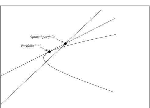
where n is uniquely determined by m (for example, if m = 0.025, then n = 1.96).4 To see the mechanics of this rule, consider the usual diagram depicting the opportunity set of available portfolios (Figure 1). Recall that the efficient set is a straight line with vertical intercept r and slope (µ*

p, t + 1– r) /σ*p, t + 1, where portfolio

“*” is the “tangency portfolio”—that is, the portfolio comprised entirely of risky assets that is defined by the point of tangency between a ray from the vertical axis (with intercept r) and the set of feasible portfolios comprised of just risky assets. Note first that the return-benchmark rule picks the portfolio located at the inter-section of the constraint (2) and the efficient set and the trade-off rule picks the portfolio located at the point of tangency between the objective function (3) and the efficient set. For the loss-constraint rule, constraint (6) traces out a straight line with intercept Rˆ and slope n. The permissible portfolios must lie on or above this line. The portfolio selection problem has an interior solution (that is, finite borrowing/lending and positive investment in risky assets) only when both of the following parametric restrictions are satisfied: Rˆ < r, and n > (µ*

p, t + 1– r) /σ*p, t + 1.

4_{The constraint (6) is equivalent to the following more common formulation in the literature discussing} VaR portfolio management rules: Prob[Vt + 1≤Vˆ ] ≤m , where there is an m percent chance of losing capital

in excess of the “value at risk,” Vˆ. As Rp,t + 1= Vt + 1/Vt, then defining Rˆ = Vˆ/Vtyields the first version of the

constraint, as presented in Telser (1955).

Figure 1. Loss–Constraint Rule

Optimal portfolio Portfolio “*” r Rˆ σp µp

Under these assumptions, there exists a unique optimal portfolio, defined by the intersection of the constraint and the linear efficient set. The optimal portfolio is therefore a linear combination of borrowing/lending and portfolio “*.”

Rebalancing Events

The paper studies portfolio rebalancing in response to two types of shocks. The first is a volatility event, which is defined as an increase in the (conditional) variance of an asset’s return. The finance literature has previously considered optimal portfolio rebalancing in response to changes in parameters of asset-return distributions (see Best and Grauer (1991a, and 1991b)), and in the contagion literature some papers have focused specifically on this type of shock (e.g., Calvo and Mendoza, 2000). The second type of shock is a capital event, defined as a reduction in Vt. Calvo

(1998, and 2000) is concerned with this type of shock in tandem with margin calls.

III. Volatility Events

To permit analytical results, it is assumed in this section that N = 2 (i.e., two risky assets).5 _{The first result characterizes portfolio rebalancing for the} return-benchmark and trade-off rules.6

Result 1. When the optimal portfolio has long positions in both risky assets and there

is positive correlation between asset returns, for both the return-benchmark and trade-off rules a volatility event for asset 2 necessarily decreases the amount invested in asset 2 and increases the amount invested in asset 1. When the correlation between asset returns is negative, these same predictions hold for the return-benchmark rule, but under the trade-off rule the amount invested in both risky assets decreases.

This result can be interpreted in terms of “income” and “substitution” effects. An increase in the risk of asset 2 effectively raises the relative price of asset 2, and thus creates an incentive to tilt the portfolio away from asset 2 and toward other assets (a substitution effect). On the other hand, any given basket of risky assets is now riskier, or “more expensive,” which reduces demand for risky assets generally (an income effect). The return-benchmark rule permits no flexibility in trading off risk and return when choosing a portfolio, so the portfolio adjustment in this case is driven by the substitution effect. With the trade-off rule, negative correlation weakens the substitution effect because diversification opportunities are significant, and thus can lead to sales of both risky assets (i.e., the income effect dominates).

How robust is result 1? First, note that increased volatility in one market could raise asset return covariances via the mechanism ct + 1= ρt + 1σ1, t + 1σ2,t + 1 (e.g., Folkerts-Landau and Garber, 1998). Thus, the question arises as to whether this

5_{Instead, one could allow for an arbitrary number of risky assets but impose additional structure on the} joint distribution of asset returns (e.g., Calvo and Mendoza, 2000). For the general case, Best and Grauer (1991a, and 1991b) discuss a technique for identifying the effects of changes in means of asset returns.

6_{Technical derivations and formal proofs are provided in the working paper version of the paper} (Schinasi and Smith, 1999).

mechanism might be a potential source of contagious selling of risky assets. The answer is that it cannot: result 1 holds regardless of whether an increase in volatility affects covariances.7

Second, only for positive correlation between asset returns does a volatility event in one asset increase the position in the other asset for both rules considered in result 1. Is this the most relevant case? Because asset returns are generally posi-tively correlated across countries, and particularly between markets in the same region, this would appear to be the reasonable case.8

Third, result 1 is a statement about an increase in one asset’s risk if everything else is the same. There is much empirical literature in finance (e.g., Haugen and others, 1991) that finds that increases in risk are associated with short-run decreases in asset prices (i.e., below-average expected returns in the short run) but higher future expected returns. It may be reasonable therefore to imagine that, at least initially, investors experience both an increase in the risk of an asset and a decrease in the expected return of the same asset. This generalization would not affect result 1 simply because asset 1 would become an even more favorable investment opportunity than asset 2.

Fourth, result 1 focuses on the case of long positions in both risky assets. If an investor had a short position in asset 2, it is straightforward to show that a volatility event in asset 2 reduces demand for asset 1 by this investor. In such cases, the volatility event causes short sellers to reduce short positions (as the asset is riskier to short sell), which tends to reduce the size of the long positions in other assets. This possibility is of some interest, but it does not explain “contagious selling of risky assets” because closing out short positions requires

purchasing the event asset.

In summary, result 1 appears to be a fairly robust prediction. The next result shows that the loss-constraint rule has more flexible properties than these other rules.

Result 2. For the loss-constraint rule, a volatility event for asset 2 necessarily

reduces the amount invested in asset 2, but increases (decreases) the amount invested in asset 1 if the parameter n is sufficiently large (small).9

7_{Specifically, result 1 holds both when the covariance is assumed invariant to the event and when the} covariance increases via the mechanism discussed in the text. Another possibility is that the correlation coefficient, ρt + 1, increases. It is straightforward to show that an increase in the correlation alone cannot

result in both asset demands decreasing, except in the case of ρt + 1< 0, and then only for the trade-off

rule, which is qualitatively exactly the same result as result 1 for a volatility event.

8_{For instance, during the period December 1991–December 1996, of 84 pairwise correlations} between dollar-denominated daily returns for 14 emerging equity markets, Kaminsky and Reinhart (1999) report that 70 are positive; and when Russia is excluded, none exceed –0.10. See also International Monetary Fund (1997).

9_{Specifically, the threshold value for n is}

An explicit expression for σ∗pis given in Schinasi and Smith (1999).

2 _{1 1 2 1 1} 2 1 1 1 2 1 1 1 1 1 2 1 2 2 1 1 µ µ σ µ σ µ µ σ µ , , *, , , , , , , t t p t t t t t t t t t r r r r c r r c + + + + + + + + + + + −

(

)

(

−

)

−

(

)

+

(

−

)

[

]

[

(

−

)

+

(

−

)

]

.

The reason the loss-constraint rule can generate selling of both risky assets is that this rule can produce greater “income effects.” The magnitude of the income effect is determined by the parameter n, which is linked to the risk tolerance of the portfolio manager—the parameter m in equation (5). Specifically, when n is small, risk tolerance is high, so small changes in the risk-return ratio have large effects on risk taking. Consequently, a volatility event, which amounts to a reduction in the expected return per unit of risk for any given portfolio, produces a large income effect and reduces the demand for risky assets generally.

In summary, when asset returns are positively correlated, the loss-constraint rule is unique among the portfolio management rules in explaining why an investor might reduce both risky asset positions due to a volatility event. This implies that there are plausible portfolio management rules that explain contagious selling of risky assets due to volatility events. The quantitative significance of this possibility is addressed in Section V.

IV. Capital Events

When “increased volatility” is associated with negative returns on existing invest-ments, then equity capital, Vt, will fall. Capital satisfies Vt = Vt –1Rp,t, and thus a

capital event (as defined above) occurs when Rp,t< 1. A capital event can be the

result of a significant loss on one position or, if there are common fundamentals, by losses on many positions. The next result isolates the effect of a capital event on the optimal scale of investment in risky assets.

Result 3. Suppose the conditional distribution of asset returns is the same in

periods t–1 and t, and a capital event (of a given magnitude) occurs in period t. Then, for all portfolio management rules:

(i) If the portfolio is not leveraged, the optimal amount invested in risky assets collectively in period t is greater than the value of the risky-asset position prior to rebalancing. Thus, there are net purchases of risky assets during period t. (ii) If the portfolio is leveraged, the optimal amount invested in risky assets collec-tively in period t is less than the value of the risky-asset position prior to rebal-ancing. Thus, there are net sales of risky assets during period t.

The assumption that the conditional distribution of asset returns is the same at the two dates implies that desired portfolio weights are the same at the two dates. Since Wt and Bt are proportional to capital, the effect of a reduction in

capital is that it alters the desired scale of investment in risky assets (Wt) and

the scale of borrowing (Bt); the portfolio weights that determine how these

amounts are split into investments in individual assets are the same as in the previous period. For the case of an unleveraged portfolio, this rebalancing process will necessarily involve reducing the position in riskless assets and increasing the position in risky assets. The reason is that, prior to rebalancing the portfolio, the value of the risky asset position will have fallen by more than capital has fallen because the latter falls by an amount equal to the loss on risky asset holdings less the income on riskless asset holdings. Thus, to reestablish

optimal portfolio weights, some of the riskless asset position must be liquidated and invested in risky assets.

For the case of a leveraged portfolio, there is also a shift away from “riskless assets,” but since this is a negative position (i.e., borrowing), rebalancing involves reducing the scale of borrowing. This is important because Wt= Vt+ Bt, and thus

a reduction in leverage must necessarily reduce the amount invested in risky assets. Note that this deleveraging process has nothing to do with margin calls (which are considered separately below), but rather stems entirely from the fact that the optimal amounts of leverage and investments in risky assets are propor-tional to equity capital. In addition, while result 3 focuses on the case of a capital event of a given magnitude, in practice leverage will also generally increase the magnitude of the capital event for a given percentage loss on the portfolio of risky assets. The reason is that individual risky asset weights are larger than for an unleveraged portfolio and thus a given percentage loss on a portfolio of risky assets generates a larger capital event. This would therefore magnify the delever-aging process. These potentially important roles of leverage are reflected in the simple example displayed in Table 1.

Result 4. Assume that the conditional distribution of asset returns is the same in

periods t–1 and t and a capital event (of a given magnitude) occurs in period t. For all portfolio management rules, the optimal amount invested in any asset is less than (greater than) the value of the position prior to rebalancing in period t if the realized return on the asset is greater than (less than) the return on the portfolio.

Rebalancing involves changing the size of each position from the amount

Ri, twiVt–1to the amount wiVt(by assumption optimal portfolio weights are the

Table 1. Leveraged Versus Nonleveraged Portfolios

Capital Risky Assets Debt

V W B

No Leverage

Initial 100 50 –50

After fall 95 40 –55 After rebalancing 95 47.5 –47.5 Net purchases of risky assets 7.5

Leverage

Initial 100 150 50

After fall 65 120 55 After rebalancing 65 97.5 32.5 Net purchases of risky assets –22.5

Notes: The calculations assume that the return on the portfolio of risky assets is –20 percent and the riskless interest rate is 10 percent.

same). Result 4 says that when a capital event of a given magnitude occurs, rebalancing tends to reduce positions in the best-performing assets and increase other positions in order to restore optimal portfolio weights. Nevertheless, if the portfolio is leveraged then an adverse shock to the realized return on the port-folio (and thus a capital event) can easily generate sales of every risky asset. To illustrate, consider another simple example. Suppose that Ri, t= 1 for i= 1, ... , N,

which implies that asset prices all turn out to be unchanged from t – 1 to t . Since

Rp,t=

Σ

N

i = 1wi,t – 1Ri,t+ w0,tr (7)

then for an unleveraged portfolio, Vt≥Vt–1(with strict inequality if there is a

positive position in the riskless asset). However, for a leveraged portfolio, it is necessarily the case that Vt< Vt–1, because w0, t< 0. Thus, there would be net

sales of every risky asset during period t and a reduction in leverage. Note that the presence of leverage itself is responsible for the capital event in this example because the returns on risky asset positions, while not negative, are simply not high enough to finance the debt. This example highlights the point made above that leverage increases the sensitivity of capital to risky asset returns.

Margin Calls

Margin is normally defined as the ratio of equity to assets (the inverse of the leverage ratio). In the preceding discussion, margin constraints are ignored. There are two types of margin constraints and two types of associated margin calls that are commonly identified in primitive securities markets: “initial” and “maintenance” margin constraints.10_{An initial margin constraint is a minimum} permissible ratio of equity to the value of the investment position when it is first established. A maintenance margin constraint is a floor on this ratio subsequent to the position being established—i.e., on a marked-to-market basis. An initial margin call is simply a requirement to put up more equity when a position is first established. In the United States, the Federal Reserve Board requires that initial margin be at least 50 percent (Regulation T). Maintenance margin requirements imposed by brokers in the United States are typically 25 percent for long positions in U.S. equity markets (they can be substantially higher or lower than this in other markets and for transactions other than long positions in primitive securities). A “maintenance margin call” is a requirement to put up more equity capital to maintain a position. The focus in this section is on this type of margin call.

10_{There are corresponding notions of initial and maintenance margin constraints in derivative} markets, although the calculation of “margin” is usually more complicated (often involving the pledging of collateral). The simple model used in this paper relates most clearly to investment and margin in prim-itive securities markets. Nonetheless, the essential intuition underlying the desire to deleverage when there are adverse shocks to capital applies to leveraged securities positions generally. The important distinction in the following discussion of margin calls is between leverage that arises simply because a financial institution makes use of debt finance, in comparison with outright leveraging of a securities posi-tion (possibly with a posiposi-tion in derivative markets).

There are two circumstances in which it is reasonable to abstract from main-tenance margin constraints. The first is when the manager has a margined position but the capital event is not big enough to cause the maintenance margin constraint to bind. As discussed above, rebalancing can lead to substantial deleveraging independently of margin calls. Thus, if one thinks about the margin constraint applied to the rebalanced portfolio, then this possibility is not as restrictive as it may appear. The second circumstance is when leverage arises for reasons other than taking outright leveraged positions in securities. This would be the case for trading portfolios of commercial and investment banks.11_{The paper next considers} maintenance margin requirements when neither of these circumstances applies.

To illustrate, consider a maintenance margin requirement at the beginning of period t, before the portfolio is rebalanced. Formally, this constraint is

(8) where β ∈[0,1]. In line with existing practice, this specification assumes that any loss or gain on the portfolio is absorbed by capital. A margin call in period t is trig-gered when (8) is violated. Specifically, a decrease in portfolio value totaling

Vt–1–Vt> 0 leads to a margin call of βBt–1/ (1–β) – Vt.12The interesting case occurs

when the margin call requires reducing the size of the risky position; that is, being forced to deleverage.13 _{In that case, a margin call totaling x would require the} liquidation of (1–β)x /βof the portfolio. As discussed above, even in the absence of maintenance margin requirements, the portfolio manager will optimally wish to deleverage when capital falls. Thus, a margin call would only matter if it leads to deleveraging beyond that which the manager would have chosen anyway. Numerical examples presented below show that a capital event will often produce a desired reduction in margin. In these cases, margin calls would not have any effect on the investor’s sales of risky assets.

Do Value-at-Risk Rules Have Unique Rebalancing Properties?

Some commentators have suggested that the loss-constraint rule, and specifically the VaR methodology, is a source of contagious selling of risky assets by financial insti-tutions that have securities portfolios.14 _{The textbook portfolio allocation model is} not suited to studying asset price dynamics under alternative portfolio management rules, but it is well suited to address the more general question of whether there are significant differences in portfolio rebalancing under alternative rules. The numerical

V V B t t+ t ≥ −1 β,

11_{The importance of general forms of leverage are discussed at length in President’s Working Group} on Financial Markets (1999).

12_{This assumes that the investor must bring the margin back up to the maintenance margin} require-ment. In some markets, the investor is required to restore margin to the initial margin requirerequire-ment. This latter possibility would generate larger margin calls than former.

13_{The alternative is simply that the manager comes up with new capital—i.e., capital injected into the} portfolio—equal to the margin call.

14_{This argument appears regularly in the financial press (e.g., The Economist, 1999 and 2000) and} has been suggested also by some in the securities business (e.g., Folkerts-Landau and Garber, 1998).

analysis in Section V provides direct quantitative evidence on this question, but at this point three general observations from the analysis above are noteworthy. First, the suggestion (e.g., The Economist, 1999 and 2000) that VaR-type portfolio manage-ment rules are unique because they imply that risky positions should be reduced when overall market volatility rises is too strong.15 _{Specifically, a general increase in} asset-return volatility will reduce risky positions under many portfolio management rules. Second, a local increase in volatility—a “volatility event,” as defined above—can lead to a general reduction in higher-risk positions under VaR rules, whereas for the other rules considered above this is not possible when asset returns are positively correlated. Nevertheless, the numerical analysis in the next section of the paper suggests that the quantitative significance of this difference between the loss-constraint rule and other rules appears to be small. Third, a capital event produces the same basic rebalancing dynamics for all of the portfolio management rules.16

V. Numerical Exercises

The numerical analysis in this section assumes that, prior to a volatility or capital event, portfolio equity capital is 100 and the moments of asset returns (in gross percentage terms) are µ1,t= 112, µ2,t= 115, r = 106, σ1,t= 8, σ2,t= 12, and ρt= 0.1.

This parameterization implies Sharpe ratios for both assets of 0.75.17 _{In practice,} Sharpe ratios calculated using realized returns lie between 0.2 and 2.0, depending on the asset (or portfolio), the time period used to compute means and standard devia-tions, and the frequency of the assumed holding period. A Sharpe ratio of 0.75 is in line with estimates for emerging equity markets and for higher-yielding bonds (e.g., IMF, 1997 and 1999). Alternative parameterizations are discussed below.

Values must also be assigned to the parameters specific to the portfolio management rules—k for the return-benchmark rule, τ for the trade-off rule, and {n,Rˆ} for the loss-constraint rule. The approach taken is to choose {k,τ,Rˆ} in order to generate specific degrees of leverage; the additional parameter for the loss-constraint rule, n, is set at 1.96. Three levels of leverage are considered: no leverage, modest leverage (a two-to-one leverage ratio), and high leverage (a four-to-one leverage ratio). The largest of these leverage ratios is reasonably high for an investor with a margined position, but is low for a financial institution.18

15_{It is not clear whether the argument pertains to banks’ internal VaR limits or to regulatory} constraints. Note, however, that regulatory capital requirements are rarely binding for most large banks. 16_{One might argue that loss-constraint portfolio management rules could have different predictions for} the nature of the rebalancing if a capital event is associated also with a change in a parameter governing the rule, namely Rˆ or m. In this context, a fair comparison of rules would require also changing the target expected return for the return-benchmark rule and the risk tolerance parameter for the trade-off rule. It is not obvious therefore that the loss-constraint rule would have unique rebalancing predictions under a capital event.

17_{The Sharpe ratio here is defined in the standard way as the mean return minus the riskless rate,} divided by the standard deviation. See Sharpe (1994) for a thorough discussion.

18_{Long Term Capital Management’s balance sheet leverage ratio was 28-to-1 at end-1997; it also had} off-balance sheet OTC derivatives positions with notional value totaling 1.3 trillion at end-1997. The average balance sheet leverage ratio of the five largest U.S. commercial bank holding companies at end-1998 was 14-to-1, while the five largest investment banks’ average leverage ratio was 27-to-1. The source for these figures is President’s Working Group on Financial Markets (1999).

The experiment involves two shocks. First, at time t the value of σ2,t + 1 increases by 50 percent. This is a substantial increase in an asset’s volatility, but it is well below observed increases in bond and equity return volatility at the onset of the crises in Asia and in Mexico (see IMF, 1998 and 1999). The second shock is a capital event at time t. Specifically, the portfolio of risky assets incurs a loss of 10 percent. As discussed above, the magnitude of the capital event caused by a 10 percent loss on the portfolio of risky assets depends on the amount of leverage in the portfolio.19_{To facilitate the interpretation of the results, it will be assumed} that this loss is accounted for entirely by asset 2 (i.e., the price of asset 1 does not change). In addition to the net effect of both events occurring simultaneously, also reported are the distinct effects of each of the volatility and capital events (see Tables 2–4).20 _{There are five observations from this exercise.}

19_{Specifically, capital at time t is given by V}

t= Vt–1[(w1,t–1R1,t+ w2,t–1R2,t) + w0,t–1r], so a 10 percent loss on the portfolio of risky assets implies that Vt= Vt–1[0.90(w1,t–1+ w2,t–1) + w0,t–1r].

20_{Consistent with the analysis in Sections III and IV, to isolate the consequences of the two events the} effect of the volatility event is calculated using period t – 1 capital, while the effect of the capital event is calculated using period t – 1 optimal asset weights. Calculating these two effects in this manner means these figures do not add up to the net effect of both events occurring simultaneously.

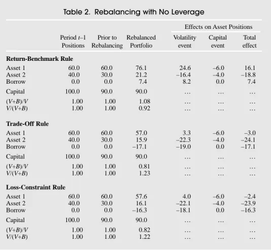
Table 2. Rebalancing with No Leverage

Effects on Asset Positions Period t–1 Prior to Rebalanced Volatility Capital Total

Positions Rebalancing Portfolio event event effect

Return-Benchmark Rule Asset 1 60.0 60.0 76.1 24.6 –6.0 16.1 Asset 2 40.0 30.0 21.2 –16.4 –4.0 –18.8 Borrow 0.0 0.0 7.4 8.2 0.0 7.4 Capital 100.0 90.0 90.0 … … … (V+B)/V 1.00 1.00 1.08 … … … V/(V+B) 1.00 1.00 0.92 … … … Trade-Off Rule Asset 1 60.0 60.0 57.0 3.3 –6.0 –3.0 Asset 2 40.0 30.0 15.9 –22.3 –4.0 –24.1 Borrow 0.0 0.0 –17.1 –19.0 0.0 –17.1 Capital 100.0 90.0 90.0 … … … (V+B)/V 1.00 1.00 0.81 … … … V/(V+B) 1.00 1.00 1.23 … … … Loss-Constraint Rule Asset 1 60.0 60.0 57.6 4.0 –6.0 –2.4 Asset 2 40.0 30.0 16.1 –22.1 –4.0 –23.9 Borrow 0.0 0.0 –16.3 –18.1 0.0 –16.3 Capital 100.0 90.0 90.0 … … … (V+B)/V 1.00 1.00 0.82 … … … V/(V+B) 1.00 1.00 1.22 … … …

First, in period t – 1 (i.e., prior to the shocks), conditional on the degree of leverage, all portfolio management rules result in nearly identical portfolios of risky assets. In addition, the loss-constraint and trade-off rules generally yield very similar asset positions both before and after the event. The rebalanced portfolio under the return-benchmark rule can, mainly for low degrees of leverage, be significantly different from the rebalanced portfolios under the other rules.21_{When there is} signif-icant leverage, however, all rules generate similar rebalanced portfolios.

Second, the volatility event alone results in a tilting of the portfolio toward the nonevent asset (results 1–2). Leverage works to magnify this effect. Recall that there are circumstances in which a volatility event causes reductions in both risky assets for the loss-constraint rule; these circumstances do not arise in this first exercise, but they will in some exercises discussed below.

Third, the volatility and capital events complement each other in producing a sharp decrease in the position in the event asset, and the capital event also works to reduce the position in the other asset. Again, these effects are magnified by leverage.

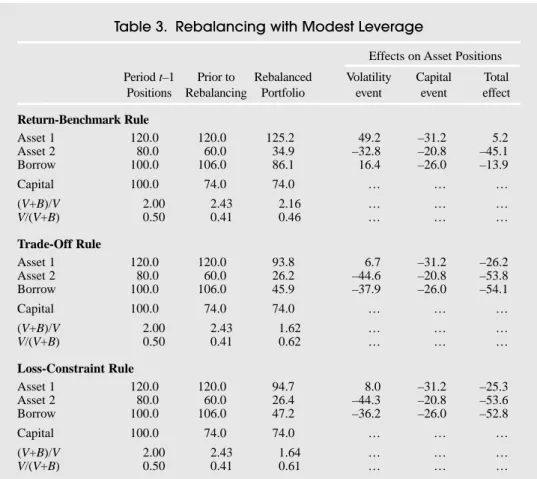
Table 3. Rebalancing with Modest Leverage

Effects on Asset Positions Period t–1 Prior to Rebalanced Volatility Capital Total

Positions Rebalancing Portfolio event event effect

Return-Benchmark Rule Asset 1 120.0 120.0 125.2 49.2 –31.2 5.2 Asset 2 80.0 60.0 34.9 –32.8 –20.8 –45.1 Borrow 100.0 106.0 86.1 16.4 –26.0 –13.9 Capital 100.0 74.0 74.0 … … … (V+B)/V 2.00 2.43 2.16 … … … V/(V+B) 0.50 0.41 0.46 … … … Trade-Off Rule Asset 1 120.0 120.0 93.8 6.7 –31.2 –26.2 Asset 2 80.0 60.0 26.2 –44.6 –20.8 –53.8 Borrow 100.0 106.0 45.9 –37.9 –26.0 –54.1 Capital 100.0 74.0 74.0 … … … (V+B)/V 2.00 2.43 1.62 … … … V/(V+B) 0.50 0.41 0.62 … … … Loss-Constraint Rule Asset 1 120.0 120.0 94.7 8.0 –31.2 –25.3 Asset 2 80.0 60.0 26.4 –44.3 –20.8 –53.6 Borrow 100.0 106.0 47.2 –36.2 –26.0 –52.8 Capital 100.0 74.0 74.0 … … … (V+B)/V 2.00 2.43 1.64 … … … V/(V+B) 0.50 0.41 0.61 … … …

21_{This difference is due to the rigidity of the return-benchmark rule: the manager has no flexibility to} trade-off risk and return on the overall portfolio.

Fourth, the magnitude of the capital event increases by a multiple of the leverage ratio and thus the associated magnitudes of asset adjustments are increasing in the leverage ratio. For instance, a 4-to-1 leverage ratio increases the magnitude of the capital event six-fold from the case of no leverage. In turn, this leads to reductions in asset positions more than 20 times larger than without leverage, and produces large sales of all risky assets. This shows that it is not difficult to generate substantial sales of all risky assets when there is leverage. In fact, with a 4-to-1 leverage ratio, sales of the nonevent asset are generally in excess of half the position, and well in excess of all of the initial capital in the portfolio. Moreover, while there are some differences in portfolio rebalancing under the three rules (particularly for the return-benchmark rule), when there is leverage these differences are of second-order importance. In particular, when there is a decrease in capital, a leveraged portfolio will be rebalanced in such a way that there are large reductions in all risky asset positions under all portfolio management rules.

Fifth, the reported leverage ratios show that, for the reasons discussed in Section IV, there is significant deleveraging—the amount borrowed to finance risky posi-tions falls. This deleveraging is central to “contagious selling” of financial assets,

Table 4. Rebalancing with High Leverage

Effects on Asset Positions Period t–1 Prior to Rebalanced Volatility Capital Total

Positions Rebalancing Portfolio event event effect

Return-Benchmark Rule Asset 1 240.0 240.0 142.1 98.4 –139.2 –97.9 Asset 2 160.0 120.0 39.7 –65.6 –92.8 –120.3 Borrow 300.0 318.0 139.8 32.8 –174.0 –160.2 Capital 100.0 42.0 42.0 … … … (V+B)/V 4.00 8.57 4.33 … … … V/(V+B) 0.25 0.12 0.23 … … … Trade-Off Rule Asset 1 240.0 240.0 106.4 13.4 –139.2 –133.6 Asset 2 160.0 120.0 29.7 –89.3 –92.8 –130.3 Borrow 300.0 318.0 94.1 –75.9 –174.0 –205.9 Capital 100.0 42.0 42.0 … … … (V+B)/V 4.00 8.57 3.24 … … … V/(V+B) 0.25 0.12 0.31 … … … Loss-Constraint Rule Asset 1 240.0 240.0 107.5 16.1 –139.2 –132.5 Asset 2 160.0 120.0 30.0 –88.5 –92.8 –130.0 Borrow 300.0 318.0 95.6 –72.5 –174.0 –204.4 Capital 100.0 42.0 42.0 … … … (V+B)/V 4.00 8.57 3.28 … … … V/(V+B) 0.25 0.12 0.31 … … …

and it does not require margin calls. In fact, with the exception of the return-bench-mark rule, the ratio of capital to assets is higher for the rebalanced portfolio, and thus margin calls would not cause any additional selling of risky assets.

These general conclusions from the numerical analysis are quite robust, particularly when leverage is present. Specifically, when leverage is present a higher positive correlation or a negative correlation between asset returns does not produce substantially different quantitative conclusions.22 _{This is also true for} alternative Sharpe ratios. Further, recall that a volatility event can generate sales of all risky assets in two cases: for the trade-off rule when there is negative corre-lation between asset returns, and it is also possible in the case of the loss-constraint rule when the parameter n is “small” (for any correlation). Experimentation with alternative parameter values designed to produce these possibilities reveals that the quantitative significance of this effect is very small in comparison to the effect of leverage when there are adverse shocks to the return on the portfolio.

VI. Conclusion

This paper takes a first pass at financial contagion by studying the predictions of the textbook model of portfolio allocation. There are three main conclusions of the analysis. First, a shock to a single asset’s return distribution may lead to a reduc-tion in other risky asset posireduc-tions. However, this result is sensitive to the portfolio management rule as well as the distribution of asset returns. Moreover, even when it occurs, the quantitative significance of contagious selling of assets due to this type of shock appears to be small. Second, the impact of an adverse shock to the return on a portfolio hinges mainly on whether or not the portfolio (or institution) is leveraged. The general conclusion is simple, but fundamental: an investor with a leveraged portfolio will reduce risky asset positions generally. This conclusion is independent of whether the leverage is margined or not; that is, it is independent of whether margin calls occur. Third, the paper considers a variety of simple port-folio management rules, and it evaluates claims that VaR rules have unique predic-tions for rebalancing. One claim is that contagion occurred after the Russian unilateral restructuring because financial institutions use VaR rules. This paper finds that VaR rules do not produce portfolio rebalancing dynamics that are very different from the other portfolio management rules considered, particularly when leverage is present.

As Calvo (1998 and 1999) and others have argued, a relatively high degree of leverage helps explain why the Russian event had greater and geographically wider financial effects than other recent events.23_{A main lesson of this paper is} that in the presence of leverage and an adverse shock to equity capital, elementary portfolio theory suggests that it is optimal to deleverage and reduce risky positions generally. This prediction is just as relevant for financial institutions that do not

22_{For details see Schinasi and Smith (1999).}

23_{The President’s Working Group on Financial Markets (1999) discusses how leverage, at both the} institutional level and in terms of margined positions, were a major factor underlying the turbulence in international financial markets during the summer and fall of 1998.

take outright leveraged positions, but instead simply finance their activities with borrowed funds, as is the case for banks and other financial institutions. This raises larger questions about the possible consequences of leverage for market dynamics and asset prices. These questions must be addressed in general equilibrium models and are therefore beyond the scope of the textbook portfolio allocation model used in this paper. This is an important topic for future research.

REFERENCES

Agenor, Pierre-Richard, and Joshua Aizenman, 1998, “Contagion and Volatility with Imperfect Credit Markets,” Staff Papers, International Monetary Fund, Vol. 45 (June), pp. 207–35. Baig, Taimur, and Ilan Goldfajn, 1999, “Financial Market Contagion in the Asian Crisis,” Staff

Papers, International Monetary Fund, Vol. 46 (June), pp. 167–95.

Best, Michael J., and Robert R. Grauer, 1991a, “On the Sensitivity of Mean-Variance-Efficient Portfolios to Changes in Asset Means: Some Analytical and Computational Results,”

Review of Financial Studies, Vol. 4, No. 2, pp. 315–42.

———, “Sensitivity Analysis for Mean-Variance Portfolio Problems,” Management Science, Vol. 37, No. 8, pp. 980–89.

Calvo, Guillermo, 1998, “Understanding the Russian Virus, With Special Reference to Latin America” (unpublished; College Park, Maryland: University of Maryland, October). ———, “Contagion in Emerging Markets: When Wall Street Is a Carrier” (unpublished;

College Park, Maryland: University of Maryland).

———, and Enrique Mendoza, 2000, “Rational Contagion and the Globalization of Securities Markets,” Journal of International Economics, Vol. 51 (June), pp. 79–113.

Chan-Lau, Jorge, and Zhaohui Chen, 1998, “Financial Crisis and Credit Crunch as a Result of Inefficient Financial Intermediation with Reference to the Asian Financial Crisis,” IMF Working Paper 98/127 (Washington: International Monetary Fund).

Folkerts-Landau, David, and Peter Garber, 1998, “Capital Flows from Emerging Markets in a Closing Environment,” Global Emerging Markets, Vol. 1, No. 3 (London: Deutsche Bank). Haugen, Robert A., Eli Talmor, and Walter N. Torous, 1991, “The Effect of Volatility Changes

on the Level of Stock Prices and Subsequent Expected Returns,” Journal of Finance, Vol. 46 (July), pp. 985–1007.

International Monetary Fund, 1997, International Capital Markets: Developments, Prospects,

and Key Policy Issues (Washington: International Monetary Fund).

———, 1999, International Capital Markets: Developments, Prospects, and Key Policy Issues (Washington: International Monetary Fund).

Kaminsky, Graciela, and Carmen Reinhart, 1999, “On Crises, Contagion, and Confusion,” forthcoming Journal of International Economics.

King, Mervyn A., and Sushil Wadhwani, 1990, “Transmission of Volatility between Stock Markets,” Review of Financial Studies, Vol. 3, No. 1, pp. 5–33.

Kodres, Laura E., and Matthew Pritsker, 1998, “A Rational Expectations Model of Financial Contagion,” Finance and Economics Discussion Series No. 1998–48 (Washington: U.S. Board of Governors of the Federal Reserve System, Division of Research and Statistics). Masson, Paul, 1998, “Contagion: Monsoonal Effects, Spillovers, and Jumps Between Multiple

President’s Working Group on Financial Markets, 1999, “Hedge Funds, Leverage, and the Lessons of Long-Term Capital Management” (Washington: Department of the Treasury, Board of Governors of the Federal Reserve System, Securities and Exchange Commission, Commodity Futures Trading Commission).

Schinasi, Garry J., and R. Todd Smith, 1999, “Portfolio Diversification, Leverage, and Financial Contagion,” IMF Working Paper 99/136 (Washington: International Monetary Fund). Available via the Internet: http://www.imf.org/external/pubs/ft/wp/1999/wp99136.pdf. Sharpe, William F., 1994, “The Sharpe Ratio,” Journal of Portfolio Management, Vol. 21, Fall,

pp. 49–58.

Telser, Lester G., 1955, “Safety First and Hedging,” Review of Economic Studies, Vol. 23, No. 1, pp. 1–16.

The Economist, 1999, “The Price of Uncertainty,” June 12. The Economist, 2000, “Bond Bombshell,” February 12.

Wolf, Holger, 1999, “International Asset Price and Capital Flow Comovements During Crisis: The Role of Contagion, Demonstration Effects and Fundamentals” (unpublished; Washington: Department of Economics, Georgetown University).

Yuan, Kathy, 2000, “Asymmetric Price Movements and Borrowing Constraints: A Rational Expectations Equilibrium Model of Crisis, Contagion, and Confusion” (unpublished; Cambridge, Massachusetts: Department of Economics, MIT).