Journal of Economic Science Research
http://ojs.bilpublishing.com/index.php/jesr
*Corresponding Author: Salvador Climent-Serrano
Department of Financial and Actuarial Economics, University of Valencia, Spain [email protected]
AbstrAct
In this research, an econometric with panel data using Ordinary least squares OLs model is constructed following the guidelines recommended by the EbA stress test methodology for 2016. the findings indicate that macroeconomic factors affecting defaults are the expected ones in the spanish credit institutions. However, loan impairments do not follow the patterns that a priori would be normal. Divergent is outcomes in defaults and impairments: the Non-Performing Loans (NPL) is pro-cyclical and impairment loss-es are counter-cyclical.
Article
econometric Model to estimate the Probability of Default and
loss Given Default in the eBA Stress test in 2016
Salvador climent-Serrano*
Department of Financial and Actuarial Economics, University of Valencia, spain
ArtIcLE INFO Article history: received: 21 November 2018 Accepted: 29 December 2018 Published: 31 December 2018 Keywords: NPL Delinquency Impairment losses spanish banks Late payment Probability of default (PD) Loss given default (LGD) Codes: JEL G21 G32 G18.
1. introduction
I
n recent years, there has been a generalized use and disclosure of the stress test. the aim is to providesecurity to financial markets, a sector that is signifi -cantly affected by rumors[1]. stress tests provide
transpar-ency to the financial market and are an important tool for
banking supervision [2]. However, their recent introduction
and the complexity of the estimations have meant that some of their objectives are not being met. For example, Quijano [3] says that the publication of the results of the 2009 bank stress test taken by the reserve had no impact on stock performance. However, the publication of the outcomes of the 2016 EU-wide stress test [4] conducted by the EbA caused a decrease of 5.1% in the European
bank-ing sector and 7.1% in the spanish bankbank-ing sector, despite having good results.
This paper focuses on this latter stress test, specifically,
on the estimation of defaults and on the losses expected from defaults in the credit portfolio of customers. the study is based on spanish credit institutions. the meth-odology will be used to develop an econometric model to estimate the probability of default (PD) and the loss given default (LGD), following the 2016 EU-Wide stress test – Methodological Note [5]. For this purpose, data from the spanish economy and spanish credit institutions are used from 2004 to 2015.
the aim is to provide a new tool for stress tests in or-der to carefully estimate losses due to the non-payment of
customer credit. These losses are usually the most signifi -cant, in terms of quantity, that credit institutions suffer.
the results may be used for supervision purposes by investors and, especially, by the credit institutions them-selves in order to estimate future losses from defaults on loans, using the methodology recommended by the EbA for calculating the losses produced in the investment port-folios of credit institutions.
2. Background and literature review
the stress testing were encouraged by the basel Accords,
whose first version was approved by the Bank for Interna -tional settlements (bIs) in 1988. based on these rules, the stress tests are a common tool in the risks management to assess the potential impact of economic [6,7,8,9].
Agreeing to til schuermann and Nyoka[10,11], one of
the consequences of the recent financial crisis is that the
ordinary methods, such as regulatory capital ratios, are no longer consistent. this lack of confidence has made
that in recent years, it has increased significantly use and
disclosure of the stress test. the goal to offer security to
financial markets, a sector that is which is very influenced
affected by rumours [1].
Investors requirement reliable information to study the opportunity of investing in a credit entities, mainly when it may be subject to loans loss provisions [12].
the analysis of the impact to loan loss provisions on
the Spanish financial system is not new and has been the
object of interest in other periods. Freixas et al. [13] studied on the period of 1973-1992 using variables such as GDP and cPI. Fernandez de Lis et al. [14] analysed the determi-nants of Default in the dates of 1963-1999 and pointed
to GDP as the most significant determinant. Delgado and
saurina [15] studied in the period 1982-2001 the GDP, interest, level of debt and asset prices in banks and sav-ings banks. More recently, Foos et al. [16] study sixteen European countries including spain, affirm that credit
growth entails an increase in loss provisions. climent and Pavia [17] study spanish credit institutions in the period of 2004-2011. Among the most relevant variables
that have had a significant impact on the increase of de -linquency are, among variables, house prices, unemploy-ment rates and property investunemploy-ment.
3. Material and Methods
3.1 Sample and Variables
the sample was chosen from just one country, spain, be-cause the peculiarities of what each country does with the data obtained from the credit institutions of one country are not optimal for the rest. Evidence of this is that the
hy-pothetical situations (scenarios) are defined independently
for each of the countries. In addition, if all countries are included, the heterogeneity of the data could offset op-posing characteristics and distort the econometric models. However, the results can be used for other countries by replicating the model and adapting it to the peculiarities of each one of them.
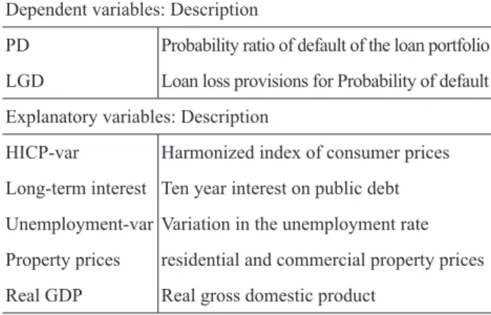
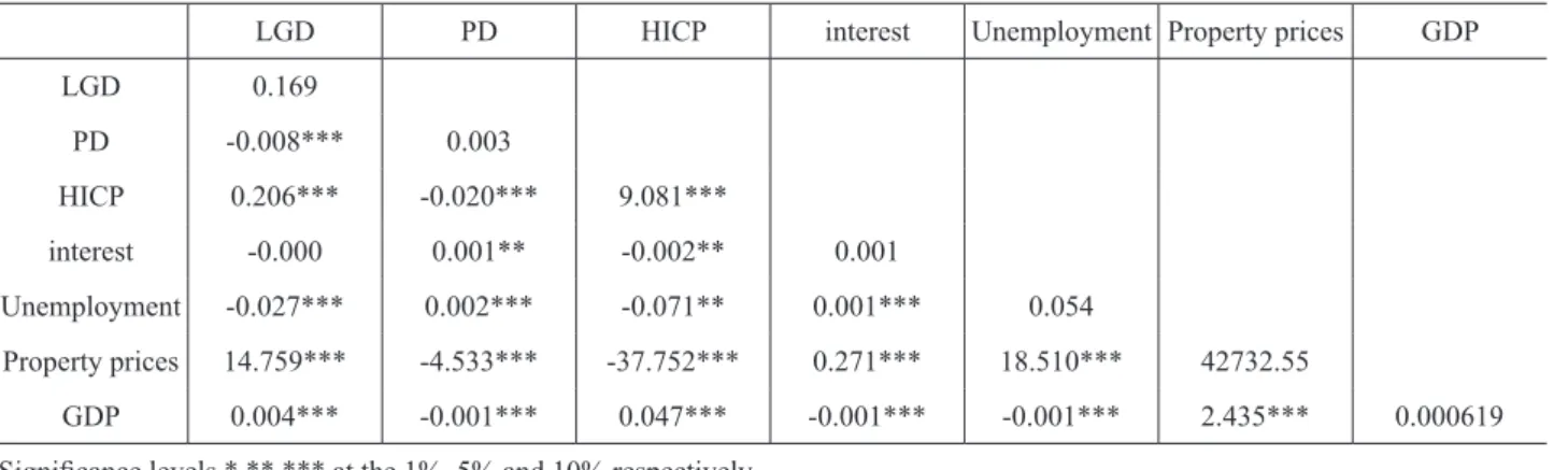
table one shows the variables used in the models and their description, And table two shows the correlation be-tween them.
table 1. Variables and Descripction Dependent variables: Description
PD Probability ratio of default of the loan portfolio LGD Loan loss provisions for Probability of default Explanatory variables: Description
HIcP-var Harmonized index of consumer prices Long-term interest ten year interest on public debt Unemployment-var Variation in the unemployment rate Property prices residential and commercial property prices real GDP real gross domestic product
3.2. empirical Methods
the methodology used is that recommended in the 2016 EU-Wide stress test - EbA Methodological Note (2016). Note 29 says: "the EU-wide stress test is conducted on the assumption of a static balance sheet." thus, the data from the credit institutions will be that which is included
in their financial statements and management report. Note
33 says: "the approach of the exercise is a constrained bottom-up stress test – i.e. banks are required to project
the impact of the defined scenarios but are subject to strict
constraints, as well as to a thorough review by competent authorities." therefore, the model will be built with the aim of allowing spanish credit institutions to estimate
im-pairment losses on loans to customers so that the authori-ties can supervise.
In the EbA methodological note 40 it states: "the esti-mation of impairments and translation to available capital requires the use of statistical methods and includes the following main steps: (i) estimating starting values of the risk parameters, (ii) estimating the impact of the scenarios on the risk parameters, and (iii) computing impairment flows as the basis for provisions that affect the P&L." Note 88 reads: "Likewise, for the estimation of projected parameters, as a general principle, banks should use mod-els rather than resort to benchmarks to determine stressed PDpit and LGDpit parameters (under both the baseline and the adverse scenario). However, banks' models will be assessed by competent authorities against minimum standards in terms of econometric soundness and re-sponsiveness of the risk parameters to ensure the model
specification results in a prudent outcome." Accordingly,
an econometric model is estimated to estimate the PDpit and LGDpit parameters. Other authors like bertsatos and sakellaris[18], also utilized dynamic and static econometric models for estimating the stress test.
the approach proposed in the 2016 EU-Wide stress test – Methodological Note EbA, (2016) to estimate the
flow of impairments on new defaulted assets at time t+1 is
given by:
Gross Imp Flow New(t+1) = Exp(t) x PDpit(t+1) x LG
-DpitNEW(t+1) Equation 1
where Exp (t) is the exposure, in our case the loans
granted to customers, PDpit(t + 1) are the NPLs caused by the exposure in year t + 1, and LGDpitNEW(t+1) are the
estimated impairment losses for the year t + 1.
therefore, two models are estimated, one for the de-faults (PD) and another for the loan impairments (LGD). the dependent variables are PD and LGD and the explan-atory variables are those that are defined in the adverse
macro-financial scenario for the EbA 2016 EU-wide bank
stress testing exercise[19]: long-term interest rates, real
GDP, HICP inflation, unemployment rate, and residential
and commercial property prices.
the data sample includes the years 2004-2015. the dependent variables, PD and LGD, were obtained from
the financial statements and management reports of prac -tically all the spanish credit institutions (banks, savings banks and credit unions), 75 different entities in the 12 periods. thus, the models are estimated using unbalanced panel data, by ordinary least squares, since not all the en-tities cover the 12 periods. For the explanatory variables we have used data from Eurostat, the bank of spain, the spanish National Institute of statistics and the Ministry of Development of spain.4
4. empirical results
Figure 1 shows the evolution of the two dependent vari-ables during the study period.
Figure 1. Evolution of the Dependent Variables In the contrasts made to the data, the unit root hypoth-esis has been accepted in two explanatory variables, the HIcP and the residential and commercial property prices. to avoid this problem, these variables have been included in the models in differences. Also, the dependent variables PD and LGD are cointegrated of order 1 c(1), so in the two models these variables will be included with a delay of one year, making the models dynamic. Furthermore, in 2012, a new financial regulation was implemented in table 2. correlation between the Variables
LGD PD HIcP interest Unemployment Property prices GDP
LGD 0.169 PD -0.008*** 0.003 HIcP 0.206*** -0.020*** 9.081*** interest -0.000 0.001** -0.002** 0.001 Unemployment -0.027*** 0.002*** -0.071** 0.001*** 0.054 Property prices 14.759*** -4.533*** -37.752*** 0.271*** 18.510*** 42732.55 GDP 0.004*** -0.001*** 0.047*** -0.001*** -0.001*** 2.435*** 0.000619
spain that greatly affected the impairment losses.① to
take account of this circumstance, a dummy variable is included in the LGD model that takes value 1 in 2012 and 0 for all other periods.
thus, two models are proposed:
𝑃𝑃𝑃𝑃𝑖𝑖𝑖𝑖=𝛽𝛽1+𝛽𝛽2𝐻𝐻𝐻𝐻𝐻𝐻𝑃𝑃𝑖𝑖+𝛽𝛽3𝑙𝑙𝑜𝑜𝑜𝑜𝑜𝑜 − 𝑖𝑖𝑡𝑡𝑡𝑡𝑡𝑡𝑖𝑖𝑜𝑜𝑖𝑖𝑡𝑡𝑡𝑡𝑡𝑡𝑖𝑖𝑖𝑖𝑖𝑖+𝛽𝛽4Unemployment𝑖𝑖
+𝛽𝛽5𝑝𝑝𝑡𝑡𝑜𝑜𝑝𝑝𝑡𝑡𝑡𝑡𝑖𝑖𝑝𝑝𝑝𝑝𝑡𝑡𝑖𝑖𝑝𝑝𝑡𝑡𝑖𝑖𝑖𝑖+𝛽𝛽6Real GDP𝑖𝑖+𝛽𝛽7𝑃𝑃𝑃𝑃𝑖𝑖,𝑖𝑖−1+𝜀𝜀𝑖𝑖𝑖𝑖 Model 1
𝐿𝐿𝐿𝐿𝑃𝑃𝑖𝑖𝑖𝑖=𝛽𝛽1+𝛽𝛽2𝐻𝐻𝐻𝐻𝐻𝐻𝑃𝑃𝑖𝑖+𝛽𝛽3𝑙𝑙𝑜𝑜𝑜𝑜𝑜𝑜 − 𝑖𝑖𝑡𝑡𝑡𝑡𝑡𝑡𝑖𝑖𝑜𝑜𝑖𝑖𝑡𝑡𝑡𝑡𝑡𝑡𝑖𝑖𝑖𝑖𝑖𝑖+𝛽𝛽4Unemployment𝑖𝑖
+𝛽𝛽5𝑝𝑝𝑡𝑡𝑜𝑜𝑝𝑝𝑡𝑡𝑡𝑡𝑖𝑖𝑝𝑝𝑝𝑝𝑡𝑡𝑖𝑖𝑝𝑝𝑡𝑡𝑖𝑖𝑖𝑖+𝛽𝛽6Real GDP𝑖𝑖+𝛽𝛽7𝐿𝐿𝐿𝐿𝑃𝑃𝑖𝑖,𝑖𝑖−1+𝜀𝜀𝑖𝑖𝑖𝑖 Model 2
In neither of the models does residual autocorrelation exist (see Figure 2).
Figure 2. residual autocorrelation
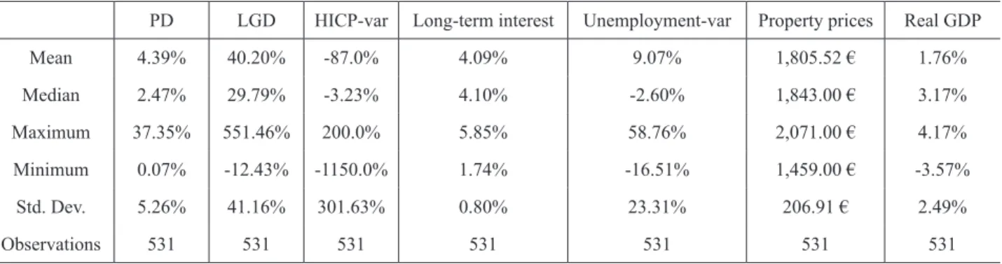
For heteroscedasticity models, they were estimated us-ing the robust method of White and cross-section weights. table 3 shows the descriptive statistics for all variables
used:
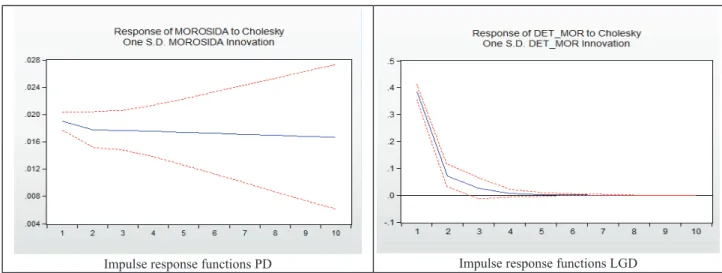
table 4 shows the Vector Autoregressive, and the table 5 shows impulse response functions
table 4. Vector autoregression
PD LGD PD(-1) 0.936 0.185988 (0.060) (0.053) [ 15.519] [ 3.475] PD(-2) 0.055 0.030 (0.068) (0.054) [ 0.813] [ 0.555] HIcP-var 0.001 -0.019 (0.001) (0.009) [ 0.120] [-2.165] Long-term interest 1.005 10.101 (0.157) (2.741) [ 6.387] [ 3.684] Unemployment-var 0.0320 -0.510 (0.004) (0.090) [ 6.515] [-5.635] Property prices -0.001 -0.001 (0.000) (0.000) [-3.639] [-1.286] real GDP -0.006 6.667 (0.112) (1.335) [-0.056] [ 4.993] Adj. r-squared 0.866921 0.257688 F-statistic 413.5758 22.98568 standard errors in ( ) & t-statistics in [ ]
PD LGD HIcP-var Long-term interest Unemployment-var Property prices real GDP
Mean 4.39% 40.20% -87.0% 4.09% 9.07% 1,805.52 € 1.76% Median 2.47% 29.79% -3.23% 4.10% -2.60% 1,843.00 € 3.17% Maximum 37.35% 551.46% 200.0% 5.85% 58.76% 2,071.00 € 4.17% Minimum 0.07% -12.43% -1150.0% 1.74% -16.51% 1,459.00 € -3.57% std. Dev. 5.26% 41.16% 301.63% 0.80% 23.31% 206.91 € 2.49% Observations 531 531 531 531 531 531 531
table 5. Impulse response functions
Impulse response functions PD Impulse response functions LGD the results of the model econometric are shown in
ta-ble 6.
table 6. Econometric models
Model 1. PD Model 2. LGD c -0.034** 1.600 (0.014) (0.360) HIcP 0.001** -2.025** (0.000) (0.010) Long-term interest 0.656*** 1.999 (0.136) (2.002) Unemployment 0.023*** -0.380*** (0.004) (0.079) Property prices 0.000 0.000 (0.000) (0.000) real GDP -0.219 6.114*** (0.143) (2.130) PD(-1) LGD(-1) 0.960*** 0.331*** (0.027) (0.030) Dummy 2012 0.394*** (0.028) Adjusted r-squared 0.938 0.784 Durbin-Watson statistic 2.084 2.206 F-statistic 1144.231 236.105
Significance levels *,**,*** at the 1%, 5% and 10% respec -tively. robust standard errors between parentheses.
the impact on PD and LGD of the variables indicated by the EbA in stress test scenarios are:
regarding the probability of default (PD), there exists
considerable inertia of the dependent variable over the next year. With regard to other variables, the increase in the long-term interest rates produces an increase in PD; the same happens with unemployment and to a much lesser extent with the HIcP. the only variable that causes a decrease in PD is the increase in real GDP, although its
significance level is 0.12. And finally, the residential and
commercial property prices variable is not statistically
significant and, in addition, its coefficient is 0.
turning to the LGD, the results are not the same, or similar. While there is also dependent variable inertia, it
is much less, the coefficient being 0.33 compared to 0.96
for the PD. the increase in the HIcP and the Unemploy-ment decreases the LGD. the dummy variable has been significant with a coefficient of 0.39. the only variable that reduces the LGD with its increase is the real GDP.
The price of housing continues with the same coefficient,
0, and is not statistically significant, with the long-term
interest not being statistically significant either.
6. Discussion
the results obtained for the PD are expected because it is logical that both the increase in unemployment and rising interest rates would involve an increase in the PD. the same happens with the real GDP; if this parameter is in-creased it is logical that the PD would decrease. However, the results obtained for the LGD are not as logical. this circumstance can be seen in Figure 1. the graph shows that when the PD increases, the LGP decreases, and there is no reason for it to be that way. In the econometric mod-el it is found that when the economy is growing (increase in real GDP and lower unemployment), the LGD grows, just the opposite of the results obtained in the model of the probability of defaults. In this case, a smoothing effect of the results occurs, agreeing with other studies [20]. It is also
significant that the level of inertia of the dependent vari-able (LGD) is three times lower than in the model of the PD. For all this we can say that the effects of the macro-economic variables are not the same in the LGD as in the PD, and they are also not the expected ones. In addition, one must take into account the possible legislative chang-es, or other events that may affect the dependent variables studied, as was demonstrated with the legislative changes of 2012.
7. Direction for Future Work
the investigation should be deepened in three areas: First-ly, in the smoothing that has been detected and its possible causes. secondly, the effects of the internal variables on the PD and LGD should be investigated, as they are likely
to have a significant effect. The PD and LGD may not be the same in solvent credit institutions with high profits as in entities in economic difficulties. Finally, it is not logical that the significant change in the price of housing does not
affect the study variables, so this aspect should also be looked into more closely.
Annotation
① this is an example of the uniqueness that each country can have.
Acknowledgment
the authors wishes to thank the support of the chair of Interna-tional Finance-banco santander.
references
[ 1 ] climent-serrano, s. stress test based on Oliver Wyman in bank of spain: an evaluation. banks and bank systems, 2016a,11 (3), 64-72.
[ 2 ] sahin, c., & de Haan, J. Market reactions to the Ecb's comprehensive Assessment. Economics Letters. http:// dx.doi.org/10.2139/ssrn.2572985.
[ 3 ] Quijano, M. Information asymmetry in Us banks and the 2009 bank stress test. Economics Letters. http://dx.doi. org/10.1016/j.econlet.2014.02.014.
[ 4 ] EbA (2016) EbA publishes 2016 EU-wide stress test re-sults. http://www.eba.europa.eu/-/eba-publishes-2016-eu-wide-stress-test-results.
[ 5 ] EbA 2016 EU-Wide stress test – Methodological Note. http://www.eba.europa.eu/documents/10180/1259315/201
6+EU-wide+stress+test-Methodological+note.pdf
[ 6 ] Huang, X., Zhou, H., & Zhu, H. A framework for as-sessing the systemic risk of major financial institutions.
Journal of banking and Finance.
doi:10.1016/j.jbank-fin.2009.05.017.
[ 7 ] Coffinet, J., Pop, A., & Tiesset, M. Monitoring financial distress in a high-stress financial world: The role of option
prices as bank risk metrics. Journal of Financial services research. DOI: 10.1007/s10693-012-0150-2.
[ 8 ] bellini, t. Integrated bank risk modeling: A bottom-up statistical framework. European Journal of Operational research. doi:10.1016/j.ejor.2013.04.031.
[ 9 ] cerutti E. & schmieder c. ring fencing and consoli-dated banks' stress tests. Journal of Financial stability. doi:10.1016/j.jfs.2013.10.003.
[10] schuermann, t. stress testing banks. International Journal of Forecasting. doi:10.1016/j.ijforecast.2013.10.003 [11] Nyoka, c. banks and the fallacy of supervision: the case
for Zimbabwe. banks and bank systems,2015, 10( 3). [12] beltratti, A. and stulz, r.M. the credit crisis around the
globe: why did some banksperform better? Journal of
Fi-nancial Economics. doi:10.1016/j.jfineco.2011.12.005
[13] Freixas Dargallo, X., De Hevia Payá, J. and Inurrieta beruete, A. Determinantes macroeconómicos de la moro-sidad bancaria: un modelo empírico para el caso español', Moneda y crédito, 1994, 199, 125-156.
[14] Fernández de Lis, s. Martínez, J. and saurina, J. crédito bancario, morosidad y dotación de provisiones para insol-vencias en España, boletín Económico banco de España, Noviembre, 2000, 1-10.
[15] Delgado, J. and saurina, J. riesgo de crédito y dotaciones a insolvencias. Un análisis con variables macroeconómi-cas, Moneda y crédito, 2004, 219, 11-42.
[16] Foos, D. Norden, L. and Weber, M. Loan growth and risk-iness of banks, Journal of banking & Finance, 2010, 34, 2929-2940
[17] climent-serrano, s. an Pavia, JM. An analysis of loan default determinants: the spanish case. banks and bank systems, 2014, 9, (4) 116- 123.
[18] bertsatos, G., & sakellaris, P. A dynamic model of bank valuation. Economics Letters, http://dx.doi.org/10.1016/ j.econlet.2016.05.014
[19] EBA Adverse macro-financial scenario for the EBA 2016
EU-wide bank stress testing exercise.
http://www.eba.eu-ropa.eu/documents/10180/1383302/2016+EU-wide+stress +test-Adverse+macro-financial+scenario.pdf .
[20] climent serrano, s., Dotaciones para los deterioros de los créditos. Un estudio por ciclos económicos. cuadernos de Economía (2016b), http://dx.doi.org/10.1016/j.ces-jef.2016.01.001.