Travel time measure specification by functional approximation: application of radial basis function neural networks

Procedia Social and Behavioral Sciences 20 (2011) 613–620

Social and

Behavioral

Sciences

www.elsevier.com/locate/procedia

14

EWGT & 26

MEC & 1

RH

Travel time measure specification by functional approximation:

application of radial basis function neural networks

Hilmi Berk Celikoglu

a _{Department of Civil Engineering, Technical University of Istanbul, Ayazaga Campus,Maslak, 34469, Istanbul, Turkey.}

Abstract

In this study, in the purpose of providing a dynamic procedure for reliable travel time specification, the performance of a neural functional approximation method is analysed. The numerical analyses are carried out on the succeeding sections of a freeway segment inputting data obtained from microwave radar sensor units located successively at the cross-sections of a freeway segment of approximately 4 km. Measurements on traffic variables, i.e., vehicle counts, speed, and occupancy, for the reference time periods are processed. The structure of the employed radial basis function neural networks are configured considering the data of a three-lane freeway segment obtained by succeeding sensors located in side-fired position. Travel time measures approximated by the neural models are compared with the corresponding field measurements obtained by probe vehicle. Results

prove neural model’s performance in representing spatiotemporal variation of flow dynamics as well as travel times. Adaptability of the proposed travel time specification procedure to real-time intelligent control systems is a possible future extension.

Keywords: travel time; traffic flow; neural networks; Intelligent Transportation System

1.Introduction

‘Travel time’ is an important performance criterion for the evaluation of transportation modes for urban trips and a major component for advanced travel information systems that provide timely and accurate information provision. Real-time traffic information, and accurately determining and predicting travel time data in particular, are important factors directly affecting dynamic route guidance systems viability. In the recent years, travel time measure has been a focal point in many studies within the frame of both traffic engineering and transportation planning. These studies have mainly concentrated on the assignment component of path choice models at macro level and on the specification of link-path flow characteristics for application solutions at micro level. The mutual point that each study’s objective possess is to determine travel times in a correct and realistic, alternatively in a reliable, manner. In this study, in the purpose of providing a dynamic procedure for reliable travel time specification, the performances of neural functional approximation methods are analysed. The innovation of the study is that with the incorporation

* Corresponding author. Tel.: +90-212-2853798; fax: +90-212-2853420.

E-mail address: [email protected].

© 2011 Published by Elsevier Ltd. Open access under CC BY-NC-ND license.

Selection and/or peer-review under responsibility of the Organizing Committee.

1877–0428 © 2011 Published by Elsevier Ltd. Open access under CC BY-NC-ND license. Selection and/or peer-review under responsibility of the Organizing Committee

of radial basis function neural network method, travel time measure is mapped by sourcing fundamental roadside measurements at successive data collecting locations and is calibrated by actual probe vehicle measurements.

In the succeeding section, a brief review on studies of travel time analysis explicitly considering neural network methods is provided following general procedures for obtaining travel times. The travel time specification problem formulation and the theoretical background of neural method applied are summarised in the third section. Information on data analysis within numerical implementations is provided in the fourth section. The conclusions drawn are presented together with the possible future extensions in the final section.

2.Review on relevant literature

Travel time is taken into account as a variable or performance measure in an extensive variety of application issues. Mainly, there are two methods for obtaining travel time: direct measurement, or estimation.

Conventional methods of measuring travel time are extremely labour intensive and the data amount to be economically collected is very limited to specify network travel time behaviour. This gave rise to the progression on the relevant technologies for travel time collection automation ranging from automatic vehicle identification to video license plate matching (Boyce et al., 1993; Turner, 1995; Liu and Haines, 1996). Aside measuring travel time, a wide variety of methods within different approaches has been being used to specify travelling times on transportation networks (Van Lint, 2008).

A number of different forecasting methods have been proposed for travel time forecasting including historic method, real-time method, time series analysis, and artificial neural networks (ANNs). Several methods of neural networks, i.e., multi-layer feed-forward neural networks (Armitage and Lo, 1994; Cheu, 1998; Park and Rilett, 1999), spectral basis neural networks (Park et al., 1999; Rilett and Park, 2001), modular neural networks (Park and Rilett, 1998), state-space neural networks (Van Lint et al., 2002 and 2005; Van Lint, 2006), are employed to provide predictions on freeway travel times. A mixed structure type of neural network travel time prediction system having a model learning function using time-series data processing is proposed by Ohba et al. (1997). Jeong and Rilett (2004) developed a neural network method incorporated travel time prediction frame to predict bus arrival time using automatic vehicle location data. Wei and Lee (2007) proposed a neural network model that specifies a functional relation between real-time traffic data and the actual bus travel times by traffic data collected from intercity buses equipped with global positioning systems, vehicle detectors along the roads, and the incident database. Developing a method for spatiotemporal data failures of traffic detectors, Wen et al. (2005) presented an analytical travel time estimation model and a recurrent neural network with grey-models for real-time travel time prediction. In comparison to approaches of ANNs, real time, and historic, the use of support vector machines for the short-term prediction of travel time is found to be a feasible alternative by Vanajakshi and Rilett (2007) when the amount of data is less or noisy.

3.Proposed travel time specification approach

The proposed approach to specify travel times depends on a functional approximation, where measurements on traffic variables, i.e., vehicle counts, speed, and occupancy, are input and probe vehicle collected sectional travel times are targeted to be approximated. Specification of link travel times from link flow and occupancy data is discussed in several works, including, the explicit consideration of a network flow model (Boyce et al., 1993), sectional travel time estimation (Takahashi and Yamamoto, 1999), travel time specification on signalized arterials in real-time based on data commonly provided by loop detectors and the signal settings (Geroliminis and Skabardonis, 2006), and arterial travel time estimation simultaneously by a virtual probe vehicle and archived traffic data (Liu and Ma, 2009). The model by Paterson and Rose (2008) draws on real-time speed, flow and occupancy data and is formulated to accommodate varying geometric conditions, the relative distribution of vehicles along the freeway, variations in speed limits, the impact of ramp flows and fixed or transient bottlenecks.

In this study, data obtained by a series of succeeding remote traffic microwave sensors is processed to map travel times measured by a probe vehicle on sections bounded by these sensors. Travel time measures approximated by the neural models are compared with the corresponding field measurements obtained by the probe vehicle.

3.1.Study area and data

Field data is obtained from four successive remote traffic microwave sensor (RTMS) units all located in side-fired position on a three-lane freeway approach of a Bosphorus strait crossing, on the Asian side of Istanbul. Measurements on traffic variables, i.e., long vehicle counts, n1(t), the rest vehicle counts, n2(t), speed, s(t), and occupancy, o(t), for the reference time period ‘t’ of three lanes labelled consecutively from 1 to 3 where lane#3 is adjacent to the median (Fig. 1).

Bosphorus strait crossing lane#1 lane#2 lane#3 An upstream sensor A downstream sensor

Figure 1 Location of successive RTMS units on schematic freeway approach to strait crossing.

Each measurement on the variables of flow per lane is obtained within two minutes period at sensors during the period 06.00-12.00 a.m. of January 25th_{, 2008. The variations of total vehicle count, speed, and occupancy measures} within two minutes period over the freeway section are respectively given in Fig. 2, Fig. 3, and Fig. 4.

Figure 3 Spatiotemporal variation of speed measures obtained at succeeding RTMS units

Figure 4 Spatiotemporal variation of occupancy measures obtained at succeeding RTMS units.

3.2.Problem formulation and numerical analysis

The success of radial basis function neural network (RBFNN) method in functional approximation is well documented in the relevant literature (Poggio and Girosi, 1989), which motivated us to evaluate its performance in freeway travel time mapping. In the following, the theory behind the RBFNN method and the analysis involving RBFNN are summarized.

3.2.1.Radial basis function neural network method

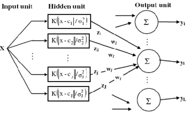
The radial basis function (RBF) neural network method, as artificial neural network, is made of three layers: a layer of input neurons feeding the feature vectors into the network; a hidden layer of RBF neurons, calculating the

outcome of the basis functions; and a layer of output neurons, calculating a linear combination of the basis functions (see Fig. 5, in which the structure of an RBFNN is shown).

Figure 5 Structure of a radial basis function neural network.

RBFNNs are generally used for function approximation, pattern recognition, and time series prediction problems. Such networks have the universal approximation property, arise naturally as regularized solutions of ill-posed problems, and are dealt well in the theory of interpolation (Poggio and Girosi, 1989). Their simple structure enables learning in stages, gives a reduction in the training time, and this has led to the application of such networks to many practical problems. The adjustable parameters of such networks are the centers (the location of basis functions), ‘cj’, the width of the receptive fields (the spread), ‘j’ the shape of the receptive field and the linear output weights. An RBFNN is a feed-forward network (Poggio and Girosi, 1989) with a single layer of hidden units, ‘x’, that are fully connected to the linear output units. Eq. 1 shows the output units, ‘j(x)’ form a linear combination of the basis (or kernel) functions, ‘K’, computed by the hidden layer nodes.

Each hidden unit output j is obtained by calculating the closeness of the input to a n-dimensional parameter vector cj associated with the jth hidden unit. K is a positive radially symmetric function (kernel) with a unique maximum at its centre cj, dropping off rapidly to zero away from the centre. Activations of such hidden units decrease monotonically with the distance from a central point or prototype (local) and are identical for inputs that lie at a fixed radial distance from the centre.

Assume that a function f: RnR1 is to be approximated with an RBF network, whose structure is given below. Let xRn be the input vector, (x, cj, j) be the jth function with centre cjRn, and width j, w=(w1, w2, …, wM)RM be the vector of linear output weights and M be the number of basis function used. We concatenate the M centres cjRn, and the widths j to get c=(c1, c2, …, cM)RnM and =(1, 2, …, M)RM, respectively. The output of the network for xRn and RM is shown in Eq. 2.



Now, let (xi, yi): i=1, 2, …, N be a set of training pairs and y=(y1, y2, …, yN)T the desired output vector, in which the superscript T denotes the vector/matrix transpose. For each cRnM, wRM, RM and for arbitrary weights i, i=1, 2, …, N, set Eq. 3. Note that i are nonnegative numbers, chosen to emphasize certain domains of the input space.











3.2.2.Radial basis function neural networks involved analysis

RBFNN travel time specification process consists of two steps, respectively the training and testing step. The prediction problem is transformed into a minimum norm problem: the search for an RBFNN to map travel time specific to each section bounded by the succeeding sensors on the freeway segment, that minimizes the Euclidean distance, P(UIk)–NN(UIk), where UIk and Yk are the actual values vector series (obtained by the four succeeding sensors), UI=[n11,1(t), n11,2(t), n11,3(t), n21,1(t), n21,2(t), n21,3(t), s1,1(t), s1,2(t), s1,3(t), o1,1(t), o1,2(t), o1,3(t), n12,1(t), n12,2(t), n12,3(t), n22,1(t), n22,2(t), n22,3(t), s2,1(t), s2,2(t), s2,3(t), o2,1(t), o2,2(t), o2,3(t), n13,1(t), n13,2(t), n13,3(t), n23,1(t), n23,2(t), n23,3(t), s3,1(t), s3,2(t), s3,3(t), o3,1(t), o3,2(t), o3,3(t), n14,1(t), n14,2(t), n14,3(t), n24,1(t), n24,2(t), n24,3(t), s4,1(t), s4,2(t), s4,3(t), o4,1(t), o4,2(t), o4,3(t)] is the input vector of NN for all four lanes, and Yk+1=P(UIk). With RBFNN method, the solution to the minimum norm problem involves a number of steps. The first one is the choice of the model inputs, and the second step is the attainment of parameters that minimize the norm given above. In order to obtain an approximation to time-varying density variable of each lane, the input variables are selected on purpose to accurately represent the flow state variation within the section bounded with succeeding sensors. Each of the long vehicle counts n1ij(t), the rest vehicle counts n2ij(t), speed measurements sij(t), and occupancy measurements oij(t) is selected as an input node, where i is the sensor label, i=1,2,3,4 and j is the counter for lane number, j=1,2,3. Therefore, the input layer of the neural network configuration consists of 48 nodes and the three output layer nodes represent the travel times specific to each section bounded by four succeeding sensors.

Since the success of an NN approximator depends heavily on the availability of a good subset of training data, data partitioning for the NN approximator is carried out considering explicitly the error term computations in all available partitions. The iterative structure of the training process needs a threshold value to stop learning; performance criteria for varying RBFNN configurations require convergence to some selected error term targets. One SSE value is targeted for RBFNN training processes. During the training stage the first half of the data set, three hours’ 2 minutes interval based collected portion, out of 180 values were analyzed, the last 90, the data of the succeeding three hours, were then used to examine the performance of the testing phase. The optimum number of training pairs has been selected considering the minima existing after the plot of MSE terms obtained by scaled training pairs. Following the training period, the networks are applied to the testing data and RBFNN performance is evaluated with the selected statistical criteria. The training vectors formed the initial centers of the Gaussian RBFs. The initial process of the training procedure was the determination of the hidden layer besides the number of nodes in the input layer, providing best training results. Because the second step is largely a trial-and-error process, and runs involving RBFNNs with hidden layer node were more than 47, any sizeable improvement in prediction accuracy is not observed. The selected number of radial basis functions for the single hidden layer was 48. The optimum spread parameter has been selected as 0.29, after the trials with the selected hidden layer node number. In the training process, 96 iterations are found sufficient with respect to the minimum SSE term obtained.

3.2.3.Simulation results

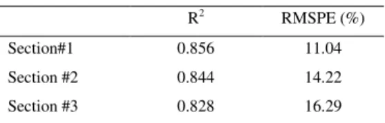
To represent the deviation of RBFNN mappings on section based travel times from section based probe vehicle measured travel times, the terms of the root mean squared percent error (RMSPE) and the coefficient of determination (R2) are calculated to evaluate statistical performance and shown in Table 1.

Table 1 Performance Criteria for Each Lane

R2 _{RMSPE (%)}

Section#1 0.856 11.04

Section #2 0.844 14.22

Section #3 0.828 16.29

The deviations of results from measurements, the RBFNN mapped travel times are plotted with the corresponding probe vehicle collected values are represented with the square of the correlation coefficient given in Table 1 for section#1, section#2, and section#3. In both periods including the minima and the maxima of the field data, the configured RBFNN provided pretty close estimates that is supported with the statistical performance criteria presented in Table 1. The results point out that the function approximation by RBFNN is close to the original

one. Efficiency of neural networks can be attributed to the capability of neural networks to capture the nonlinear dynamics and generalize the structure of the whole data set. During the mapping of travel time measure from the input vehicle count, speed, and occupancy variables, the nonlinear relationship of traffic flow variables and traversal time along the sections bounded by successive sensors on the freeway segment are modelled more appropriately with utilizing nonlinear transfer functions in the nodes of the hidden layer of neural network configuration.

4.Conclusions

Neural network estimating method, whose theoretical background is quite different, is able to provide accurate travel time measures consistent with the spatiotemporal nature of this performance variable. Considering the simulation trials and calculated statistical performance criteria, it is seen that approximating with radial basis functions leads to significantly considerable predictions. This is due to RBF’s flexibility to adapt to nonlinear traffic flow relationships. Following the process of the non-linearity in the neurons of hidden layer, the linear filtering is applied by the summing up nodes in the output layer.

Neural networks have a distributed processing structure in which each individual processing unit or the weighted connection between two units is responsible for one small part of the input-output mapping system. Therefore, each component has no more than a marginal influence with respect to the complete solution. As a result, the neural mechanism will still function and generate reasonable mappings where travel time measure is being perceived as a crucial performance evaluation criterion in the analysis of transportation systems. The adaptation of neural network methods to real-time estimation tools in the purpose of specifying appropriate measures for information dissemination and traffic management is the main future research direction in dynamic network traffic modeling. References

Armitage, W., Lo, J.-C., (1994). Enhancing the robustness of a feedforward neural network in the presence of missing data. Proceedings of the 1994 IEEE International Conference on Neural Networks and IEEE World Congress on Computational Intelligence. 2, 836-839.

Boyce, D., Rouphail, N., Kirson, A., (1993). Estimation and measurement of link travel times in the ADVANCE project. Proceedings of the IEEE - IEE Vehicle Navigation & Information Systems (VNlS) Conference 1993, Ottawa, 12-15 Oct. 1993, pp. 62-66.

Cheu, R. -L., (1998). Freeway traffic prediction using neural networks. Proceedings of the International Conference on Applications of Advanced Technologies in Transportation Engineering 1998, ASCE, Reston, VA, USA, 247-254.

Geroliminis, N., Skabardonis, A., (2006). Real time vehicle reidentification and performance measures on signalized arterials. Proceedings of the 2006 IEEE Intelligent Transportation Systems Conference (ITSC '06), 188-193.

Jeong, R., Rilett, R., (2004). Bus arrival time prediction using artificial neural network model. Proceedings of the 7th International IEEE Conference on Intelligent Transportation Systems, 3-6 Oct. 2004, pp. 988-993.

Liu, H. X., Ma, W., (2009). A virtual vehicle probe model for time-dependent travel time estimation on signalized arterials. Transportation

Research Part C: Emerging Technologies, 17 (1), 11-26.

Liu, T. K., Haines, M. (1996). Travel time data collection field tests-lessons learned. Report FHWA PL-96-010, FHWA, US Department of Transportation, Cambridge, Mass, 1996.

Ohba, Y., Koyama, T., Shimada, S., (1997). Online-learning type of traveling time prediction model in expressway. Proceedings of the IEEE Conference on Intelligent Transportation System (ITSC97) 1997, 9-12 Nov. 1997, 350-355.

Park, D. J., Rilett, L. R., (1998). Forecasting multiple-period freeway link travel times using modular neural networks. Transportation Research

Record, 1617, 163-170.

Park, D. J., Rilett, L., (1999). Forecasting freeway link travel times with a multilayer feed-forward neural network. Computer Aided Civil and

Infrastructure Engineering, 14 (5), 357-367.

Park, D., Rilett, L., Han, G., (1999). Spectral basis neural networks for realtime travel time forecasting. ASCE Journal of Transportation

Engineering, 125 (6), 515-523.

Paterson, D., Rose, G., (2008). A recursive, cell processing model for predicting freeway travel times. Transportation Research Part C:

Emerging Technologies, 16 (4), 432-453.

Poggio, T., Girosi, F., (1989). A theory of networks for approximation and learning. MIT Al Memo, no. 1140, MIT Press, Cambridge.

Rilett, L. R. & Park, D., (2001). Direct forecasting of freeway corridor travel times using spectral basis neural networks. Transportation Research

Record, 1752, 140-147.

Takahashi, Y., Yamamoto, K., (1999). Travel time information system and its operation. Proceedings of the 1999 IEEE/IEEJ/JSAI International Conference on Intelligent Transportation Systems, 5-8 Oct. 1999, pp. 944-949.

Turner, S. M., (1995). Advanced techniques for travel time data collection. Proceedings of 6th IEEE International Vehicle Navigation and Information Systems Conference (VNIS) 'A Ride into the Future' in conjunction with the Pacific Rim TransTech Conference, 30 July-2 Aug. 1995, 40-47.

Van Lint, J. W. C., (2006). A reliable real-time framework for short-term freeway travel time prediction. ASCE Journal of Transportation

Engineering, 132 (12), 921-932.

Van Lint, J. W. C., (2008). Online learning solutions for freeway travel time prediction. IEEE Transactions on Intelligent Transportation

Systems, 9 (1), 38-47.

Van Lint, J. W. C., Hoogendoorn, S. P., Van Zuylen, H. J., (2002). Freeway travel time prediction with state-space neural networks-Modeling state-space dynamics with recurrent neural networks. Transportation Research Record, 1811, 30-39.

Van Lint, J. W. C., Hoogendoorn, S. P., & Van Zuylen, H. J., (2005). Accurate travel time prediction with state-space neural networks under missing data. Transportation Research Part C: Emerging Technologies, 13 (5-6), 347-369.

Vanajakshi, L. & Rilett, L. R., (2007). Support Vector Machine technique for the short term prediction of travel time. Proceedings of the 2007 IEEE Intelligent Vehicles Symposium, Istanbul, Turkey, June 13-15, 2007, 600-605.

Wei, C. H. & Lee, Y., (2007). Development of freeway travel time forecasting models by integrating different sources of traffic data. IEEE

Transaction on Vehicular Technology, 56 (6), 3682-3694.

Wen, Y-H., Lee, T-T., & Cho, H-J. , (2005). Hybrid models toward traffic detector data treatment and data fusion. Proceedings of the 2005 IEEE Networking, Sensing and Control, 19-22 March 2005, pp. 525-530.