Robust Multi-Modal Optimisation

(1)

Khulood Alyahya

[email protected] University of Exeter, EX4 4QF, UK

Kevin Doherty

Ozgur E. Akman

Jonathan E. Fieldsend

∗

ABSTRACT

Robust and multi-modal optimisation are two important topics that have received significant attention from the evolutionary computa-tion community over the past few years. However, the two topics have usually been investigated independently and there is a lack of work that explores the important intersection between them. This is because there are real-world problems where both formulations are appropriate in combination. For instance, multiple ‘good’ solutions may be sought which are distinct in design space for an engineering problem – where error between the computational model queried during optimisation and the real engineering environment is be-lieved to exist (a common justification for multi-modal optimisation) – but also engineering tolerances may mean a realised design might not exactly match the inputted specification (a robust optimisation problem). This paper conducts a preliminary examination of such intersections and identifies issues that need to be addressed for further advancement in this new area. The paper presents initial benchmark problems and examines the performance of combined state-of-the-art methods from both fields on these problems.

CCS CONCEPTS

•Theory of computation→Evolutionary algorithms; • Com-puting methodologies→Uncertainty quantification;

KEYWORDS

Robust optimisation; uncertain optimisation; multi-modal optimi-sation.

ACM Reference Format:

Khulood Alyahya, Kevin Doherty, Ozgur E. Akman, and Jonathan E. Field-send. 2018. Robust Multi-Modal Optimisation. InGECCO ’18 Companion: Genetic and Evolutionary Computation Conference Companion, July 15–19, 2018, Kyoto, Japan.ACM, New York, NY, USA, 8 pages. https://doi.org/10. 1145/3205651.3208258

∗_{Corresponding author}

Permission to make digital or hard copies of all or part of this work for personal or classroom use is granted without fee provided that copies are not made or distributed for profit or commercial advantage and that copies bear this notice and the full citation on the first page. Copyrights for components of this work owned by others than the author(s) must be honored. Abstracting with credit is permitted. To copy otherwise, or republish, to post on servers or to redistribute to lists, requires prior specific permission and/or a fee. Request permissions from [email protected].

GECCO ’18 Companion, July 15–19, 2018, Kyoto, Japan

ACM ISBN 978-1-4503-5764-7/18/07. . . $15.00 https://doi.org/10.1145/3205651.3208258

1 INTRODUCTION

Decision makers in design situations often prefer to have multi-ple good (or optimal) solutions available before making a final selection, a famous example of this is the Second Toyota Paradox [15]. There are various reasons why returning multiple distinct high-quality solutions to the problem owner may be advantageous in real-world applications. Designs which are of the same/similar quality but are markedly different in composition can offer useful insight to the problem owner of the particular problem being solved. They also provide mitigation against a number of implementation risks such as: (1) some designs may not be directly/easily machin-able; (2) sourcing components through the supply chain/required factory configurations/additional machinery requirements impose additional costs not initially envisaged; and (3) the computational emulator of the cost function may be in error in certain regions, thereby assigning some designs misleading quality during optimisa-tion. Note that point (3) assumesembodiedoptimisation is not being undertaken, as in e.g. [13], which would remove this particular risk, but is often a relativelyexpensiveoptimisation route.

When multiple, distinct, good solutions are sought, the problem is often cast as a multi-modal optimisation problem. Here, given the feasible search domainX, and a local neighbourhood functionN(x), which returns the neighbours of ad-dimensional putative designx, multi-modal optimisation seeks to return all high quality designs which are also optimal in their neighbourhood (here ‘high quality’ may be defined in terms of global quality, or some quality threshold). Intuitively, we can think of such optimisers as trying to find the highest peaks in the fitness landscape. Multi-modal optimisation has been an active research area in the evolutionary computation (EC) community for a number of years now, with multi-modal optimisation competitions (cast in terms of finding multiple distinct global optima) running in a number of major conferences, and large enough to require recent survey papers, see e.g. [10].

By contrast, robust optimisation deals with problems where the realised performance of a design isuncertain. This may be e.g. due to operating conditions varying (for instance an aircraft wing has to perform well in a number of different environments and conditions), or may be due to machining tolerances leading to variations in manufactured designs (and therefore variation in performance). In these situations the task is to find a design whose observed performance isrobustto the source of variation experienced in the problem. This may be in terms of worst case expected performance, average performance, etc. As with multi-modal optimisation, the robust optimisation area has proved fruitful for the application of EC approaches, and various test problems have been developed

(2)

over the years, alongside the real-world application of developed algorithms.

Curiously, the combination of both problems does not appear to have been tackled. Such real-world problems, however, do in-variably exist in many engineering design situations. This paper proposes initial benchmark problems for robust multi-modal opti-misation and evaluates the effectiveness of some state-of-the-art multi-modal optimisers on these problems – both when applied in an unmodified fashion, and when augmented with techniques used for robust optimisation.

2 EXPERIMENTAL SETUP

As a first study of the intersection between the two topics of robust and multi-modal optimisation, we integrate existing methods from the robust field into multi-modal optimisation algorithms. We test their performance on modified standard benchmarks from both fields. Specifically, we examine the performance of two algorithms from the field of evolutionary multi-modal optimisation which have previously been ranked first in the IEEE CEC and GECCO “Niching Methods for Multimodal Optimization" competitions: the covariance matrix self-adaptation with repelling subpopulations algorithm (RS-CMSA) [2] and the niching migratory multi-swarm optimiser (NMMSO) [4].1According to [2], RS-CMSA is the most successful method on the CEC2013 benchmark problems [9] and the second best optimiser is NMMSO. The NMMSO algorithm has an interesting property – that of keeping track of all the modes as opposed to keeping track of only the best mode seen so far, which may prove useful when applied to the intersection of the two fields. This property is particularly appealing since in robust settings, the algorithm does not usually possess full information on the robust landscape, instead having only a noisy approximation to it (thereby inserting error into the quality evaluation of a mode).

There are various different robust quality measures used in the literature, including worst case performance and 95% confidence. Here we use the popular expected fitness measure, which we refer to as theeffective fitness, and aim to maximise. When the underlying distribution of the disturbance is known, we can write theeffective fitnessasfeff(x)=

∫∞

−∞f(x+δ)pdf(δ)dδ, where pdf(δ)is the

proba-bility density function of the disturbanceδ. Unfortunately, for most practical problems an approximation must be made via numerical integration for bounded disturbance, and where the function eval-uation budget is limited, Monte Carlo sampling to estimate this quality value becomes computationally infeasible. Instead various approaches have been developed in the literature to exploit and weight the previously evaluated designs in the disturbance set of a proposed new design, along with determining new samples to improve the estimate offeff(x), ˆfeff(x), used by an optimiser to assign

the estimated robust quality to a design.

For both MMO algorithms, we incorporate the most recent ro-bust optimisation method for generating ˆfeff(x), namely archive

sample approximation (ASA) [3]. As with many of the robust meth-ods [8, 12], ASA exploits the archive of already visited solutions to obtain a more accurate estimate offeff. ASA works by taking

Latin hypercube samples (LHS), referred to as reference points, in the disturbance neighbourhood of a solution, and the one that 1_{See e.g. http://www.epitropakis.co.uk/gecco2017/ for competition details.}

minimises the Wasserstein distance between the disturbance neigh-bourhood set and the target disturbance distribution is evaluated to update the estimate offeff[3]. The points in the disturbance set are

then weighted by the number of their reference point’s neighbours. RS-CMSA and NMMSO augmented with ASA works in exactly the same way as their original versions apart from replacingf(x) with ˆfeffwhich is obtained using ASA, and keeping an archive of

all visited solutions for RS-CMSA. To better quantify the effect of equipping the algorithms with an explicit mechanism for handling robust optimisation (i.e. ASA), we ran both algorithms without ASA and report the results obtained for these control experiments.

2.1 Test Problems

We study 13 test functions with different landscape properties, both in relation to robustness and to multi-modality (see Table 1). All problems are maximisation problems. Figure 1 shows visualisations of the original test functions together with the transformed land-scapes obtained after applying the disturbance distributions spec-ified in Table 2. For additional visualisations of the test problems up tod =3, see the online supplementary material (http://pop-project.ex.ac.uk). Test functions TP1-4 are inverted versions of their original definitions in the robust literature, and are defined below. TP1: f1(x)=− d Õ i=1 Q1(xi), x∈ [−2,2]d where Q1(xi)=                    (x_i+1)2−1.4+0.8|sin(6.283x_i)| ,−2≤x_i <0, −0.6·2−8|xi−1|−0.958887+0.8|sin(6.283x_i)| ,0≤x_i ≤2, 0 ,otherwise. TP2: f2(x)=− d+ d Õ i=1 Q2(xi) ! , x∈ [0,10]d where Q2(xi)=2 sin(10e−0.2xix_i₎e−0.25xi. TP3: f3(x)=_d1 d Õ i=1 Q3(xi), x∈ [0,1]d where Q3(xi)=                    exp −2 ln(2)xi−0.1 0.8 2 |sin(5πxi)|0.5 ,0.4<xi ≤0.6 exp −2 ln(2)xi−0.1 0.8 2 sin6(5πxi) ,otherwise. TP4: f4(x)=_d1 d Õ i=1 Q4(xi), x∈ [0,1]d,

(3)

-2 -1 0 1 2 0 0.5 1 1.5 2 (a) TP 1 0 2 4 6 8 10 -3 -2 -1 0 1 (b) TP 2 0 0.2 0.4 0.6 0.8 1 0 0.5 1 (c) TP 3 0 0.2 0.4 0.6 0.8 1 0 0.2 0.4 0.6 (d) TP 4 0 10 20 30 0 50 100 150 200 (e) TP 5 0 0.2 0.4 0.6 0.8 1 0 0.5 1 (f) TP 6 0 0.2 0.4 0.6 0.8 1 0 0.5 1 (g) TP 7 (h) TP 8 (i) TP 9 (j) TP 10 (k) TP 11 (l) TP 12 _{(m) TP 13}

Figure 1: Test functions in 1-D and 2-D. Original and robust (effective) landscapes are plotted, together with the global optima (purple squares on the original landscape; red stars on the robust landscape). In 1-D, the original landscape is plotted with a blue-dashed line and the robust landscape with a solid black line. In 2-D, the original and robust landscapes are plotted as upper and lower panels respectively, with the global optima for both landscapes marked on each plot.

where Q4(xi)=              0.5 exp−0.5(xi−0.4)2 0.052 ,xi <0.4696; 0.6 exp −0.5(xi−0.5)2 0.022 ,0.4696≤x_i ≤0.5304; 0.5 exp−0.5(xi−0.6)2 0.052 ,otherwise.

TP1-2 have been taken from [3], and test problems TP3-4 from [12].2We have modified the disturbances used for test functions 2_{Note that our definitions of TP1-4 fix typographical errors in [3, 12].}

(4)

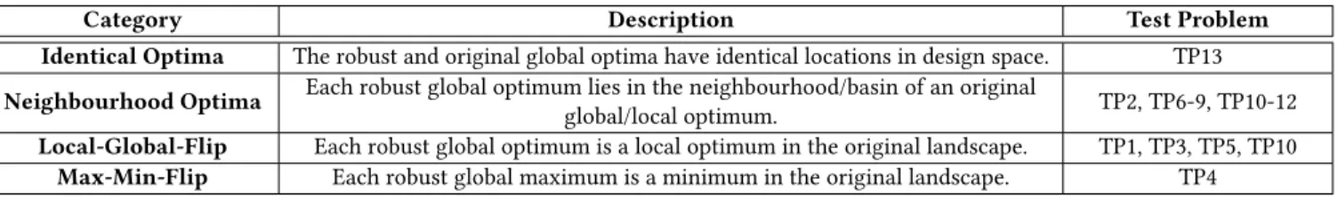
Table 1: Different test problem categories with respect to the difference between the robust and original landscapes.

Category Description Test Problem

Identical Optima The robust and original global optima have identical locations in design space. TP13 Neighbourhood Optima Each robust global optimum lies in the neighbourhood/basin of an original

global/local optimum. TP2, TP6-9, TP10-12

Local-Global-Flip Each robust global optimum is a local optimum in the original landscape. TP1, TP3, TP5, TP10 Max-Min-Flip Each robust global maximum is a minimum in the original landscape. TP4

TP3-4 by modifying the disturbance bounds and changing the dis-tributions from truncated normal distribution to uniform in order to generate robust landscapes with different properties. TP1-4 have rugged landscapes with local optima in both the original and robust functions. They become more difficult to optimise with increased ddue to the scale-up in the number of local optima. In TP1 and TP3, a local-global flip occurs where the global optimum of the robust function is a local optimum in the original function. In TP2, a weaker type of local-global flip occurs, in which the global opti-mum of the robust function lies in the the basin of a local optiopti-mum in the original function. In TP4, a max-min flip occurs where the global maxima of the robust function are minima of the original function. Note that for TP2 and TP3, since the robust optimum lies directly over a local optimum in the original function – which has a much wider basin than the original global optimum – it may be found without the use of robust optimisation measures, if the search algorithm is incapable of detecting the narrow global basin during its exploration of the design space.

TP5-13 are taken from the widely used standard multimodal benchmarks collated in the IEEE CEC2013 special session on multi-modal optimization [9]. TP5 is the Five-Uneven-Peak Trap function, TP6 is the Equal Maxima function, TP7 is the Uneven Decreasing Maxima function, TP8 is the Himmelblau function, TP9 is the Six-Hump Camel Back function, TP10 is the Shubert function, TP11 is the Vincent function, and TP12 and TP13 are the Modified Rastrigin function but with different disturbance distributions (see below). A detailed description of TP5-13’s landscape properties can be found in [9]. We applied different disturbance distributions to these func-tions to transform them into robust problems. Not all distribufunc-tions implemented were symmetric: for example we used a corner dis-turbance with TP6-TP12 to shift the location of each robust global optimum to either a local optimum in the original landscape or to the attraction basin of the original global optimum. We applied two different disturbances to the Modified Rastrigin function: a corner disturbance distribution for TP12 and a symmetric one for TP13, in order to generate two test problems with different robustness categories. The symmetric disturbance in TP13 maintains the same optima properties in the original landscape, including their location, but reduces the objective values across the entire search space.

A summary of the different robust test problem categories is shown in Table 1. The categories are adapted directly from [12]. The parameters used for each test problem, including the disturbance distribution, are presented in Table 2. Note that we truncated the disturbance for solutions with disturbance region exceeding the problem boundaries.

2.2 Parameter Settings

We took the most recent available author implementations of RS-CMSA3 and NMMSO4. We modified the implementation of RS-CMSA to keep an archive of all visited solutions, and updated NMMSO to include the extra sampled points in its search history archive. For both algorithms, we used the default parameters from their original publications [2, 3]. The size of the Latin hypercube sample used in ASA was fixed at 3d following the settings used in [3], with a maximum value of 35 ford ≥ 5. The remaining parameter settings, including the different values of the problem dimensiondand the maximum number of function evaluations, MaxEval, are shown for each problem in Table 2. We executed 30 runs of each algorithm on each test problem.

3 RESULTS

To examine the behaviour of the different algorithms during the run, we report snapshots of the results achieved at the following time points: 10−2×MaxEval, 10−1×MaxEval, and when MaxEval has been reached. We report the peak ratio [9], the bestfeff, and the

absolute error achieved by the algorithms [3]. The peak ratio (PR) is defined as PR=_G1

rR ÍR

i=1дi, whereGr is the number of known

robust global optima,Ris the number of runs, andдiis the number of robust global optima identified in theith run (given a particular quality toleranceϵ). For each run, robust global optimaдiare identi-fied using a modiidenti-fied version of the algorithm in [9], by calculating the truefeffof the modes returned. The truefeffof a given solution

is obtained via numerical integration. The absolute error (AE) is defined as AE= _|_M1_|Í m∈M feff(m) −fˆeff(m)

, whereMis the set of

modes returned by the algorithm and|M|denotes set cardinality. We report these measures over the 30 runs executed using median and median absolute deviation (MAD) as alternatives to mean and standard deviation, as the former pair is less sensitive to outliers and gives a more robust measure of the variability [5]. Statistical analyses were performed using the single-tailed Wilcoxon rank-sum test (with a 5% significance level) and corrected for multiple comparisons using the Holm-Bonferroni method (also known as the sequentially rejective Bonferroni test) [6], as it is has more statistical power than the widely used Bonferroni correction.

Table 3 shows the bestfeffout of all the returned modes and Table

4 shows the AE5. Interestingly, when considering thefeffof the

best ˆfeff, on a number of problems a better solution is found earlier

in the run snapshot, which then progressively degrades due to the 3_{Version 1.3 https://www.coin-laboratory.com/codes.}

4_{Git commit version 12, https://github.com/fieldsend/ieee_cec_2014_nmmso/.} 5_{Note that results for TP1-4 with}_d₌_{1 are available in the online supplementary}

(5)

Table 2: The test functions and their parameters. The first four problems are adapted from standard robust benchmarks and the remainder are adapted from the CEC2013 special session on multimodal optimization [9]. The three distances shown can be used in designing new performance measures. The niche radiusris only used for post-processing of the results.

d δ minimum distance r # global optima MaxEval

Original Robust

Original-Robust Original Robust

TP1 2, 5, 10 δ∼U(−0.2,0.2) - - √d4 √ d0.01 1 1 _d₌ 2, 104 d=5, 2.5×104 d=10, 5×104 TP2 2, 5, 10 δ∼U(−1,1) - - √d10.76 √d0.01 1 1 TP3 2, 5, 10 δ∼U(−0.05,0.05) - - √d0.15 √d0.01 1 1 TP4 2, 5, 10 δ∼U(−0.06,0.06) - √d0.009 √d0.002 √d0.005 1 2d TP5 1 δ∼U(−3,3) 30 - 7.5 0.01 2 1 5×104 TP6 1 δ∼U(0,0.1) 0.2 0.2 0.05 0.01 5 5 TP7 1 δ∼U(0,0.05) - - 0.14 0.01 1 1 TP8 2 δ∼U(−2.4,0) 3.89 - 1.39 0.01 4 1 TP9 2 δ_δx∼U(0,1.14), y ∼U(0,0.66) 1.44 1.42 0.22 0.5 2 2 TP10 2 δ∼U(−2,0) 0.88 4.13 2.3 0.5 d3d 3d 2×105 TP11 2 δ∼U(0,0.975) 0.29 - 0.67 0.01 6d 1 TP12 2 δ∼U(−0.1,0) 0.25 0.25 0.07 0.1 12 12 TP13 2 δ∼U(−0.05,0.05) 0.25 0.25 0 0.1 12 12

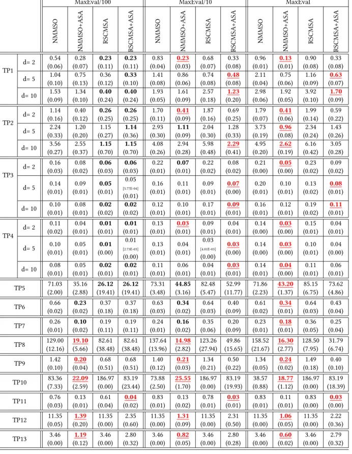
landscape pulling the algorithm away from the robust solution.6 NMMSO+ASA achieves best AE performance on 16 of the 21 test problems. The algorithm attains highestfeffon 9 test problems when

considering all returned modes, but not when considering thefeff

of the best returned ˆfeff. The case is different for RS-CMSA+ASA,

which achieves highestfeffon 3 test problems when considering

thefeffof its best ˆfeff, but does not achieve the highestfeffon any

of the problems when consideringfeffof all of the returned modes.

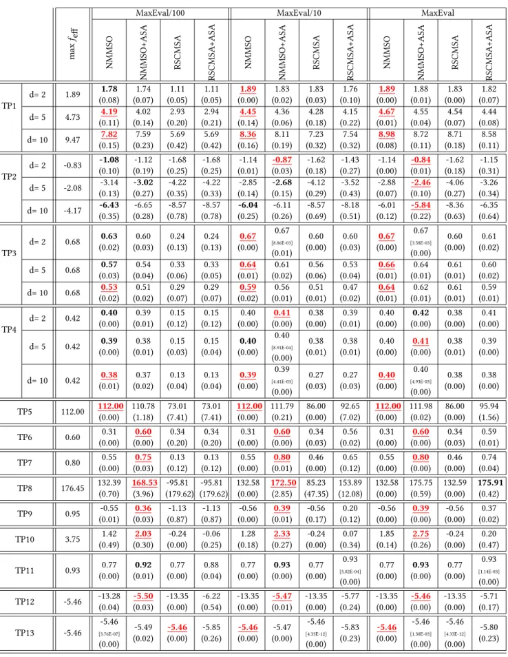
We note that without any added measures for robust optimisation, NMMSO is able to achieve bestfeffperformance on 9 of the test

problems when considering all returned modes (see Table 3). This is likely due to its mechanism of keeping track of all modes visited – this enables the algorithm to locate a greater number of local optima in the original landscape. It is thus not surprising that the algorithm achieves the bestfeffon all of the problems in the identical

optima and local-global-flip categories, apart from TP10, which is likely due to the narrow basins of local optima in this problem.

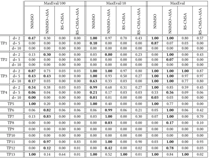
Table 5 shows the PR values obtained with accuracy levelϵ=0.1 from maxfeff7. RS-CMSA and NMMSO are able to find all robust

optima of TP13, which is not surprising given that the problem is of the identical optima category. We also note that NMMSO and NMMSO+ASA achieve the highest PR values on all but four of the test problems, namely TP9-10 and thed =10 versions of TP1-2. Indeed, none of the algorithms considered in this paper were able to find the robust optima of these four landscapes.

4 DISCUSSION

The crossover between robust and multi-modal optimisation raises a number of issues and areas worthy of further research. Perhaps 6_{See the online supplementary material, which reports the}_feff_{of the best ˆ}_feff_returned

by each algorithm on each test problem.

7_{For results obtained with}_ϵ₌₁₀−2_,₁₀−3_,₁₀−4_and₁₀−5_{, see the online}

supplemen-tary material.

the two most important issues to be addressed are: (i) the need for new benchmark problems, inspired by real-world applications with domain-specific robustness categories (e.g. computational biology problems, for which there are no general results regarding how the number of optima scale with problem dimension etc.); and (ii) the concomitant need for new performance measures quantifying the success of a given algorithm in locating robust optima in these new landscape classes. Here, we have introduced some initial bench-marks composed of a modified combination of test problems from both fields, but recognise that this is initial work in this interface domain. There already exist a number of multi-modal test problem generators that yield tunable test functions with desirable prop-erties, such as regular and irregular distributions of optima and a controllable number of global and local optima [1, 14]. One way to develop good benchmarks for this new field would be to adapt such generators to generate versatile robust multi-modal functions that fall under the different robust categories shown in Table 1.

Various performance measures are proposed and used in the multi-modal-optimisation field; however, most of these measures require prior knowledge of the number of optima, their locations in the design space, and their objective values [10]. These require-ments are usually difficult to satisfy when robust settings are con-sidered, since the transformation of the original landscape (when the disturbance distribution is known) involves integrating the function; in most cases, this is analytically intractable and accurate numerical integration is limited to a small number of dimensions. Thus, requiring prior knowledge of the properties of all optima (or global optima) could limit the design of benchmarks to easy separable problems or non-separable problems with smalld. The importance of performance measures that do not require any prior knowledge of the number of optima or their properties is not only a challenge for assessing the performance of robust-multimodal

(6)

Table 3: Median and MAD values (brackets) for the bestfeffof all returned modes. The highest feffvalue for each problem in

each snapshot is marked in bold. Results that are significantly better than all other results are underlined and marked in red. Note that all values are rounded. The difference between equal best medians due to rounding is shown in square brackets.

max

feff

MaxEval/100 MaxEval/10 MaxEval

NMMSO NMMSO+ASA RSCMSA RSCMSA +ASA NMMSO NMMSO+ASA RSCMSA RSCMSA +ASA NMMSO NMMSO+ASA RSCMSA RSCMSA +ASA TP1 d= 2 1.89 1.78 (0.08) 1.74 (0.07) 1.11 (0.05) 1.11 (0.05) 1.89 (0.00) 1.83 (0.02) 1.83 (0.03) 1.76 (0.10) 1.89 (0.00) 1.88 (0.01) 1.83 (0.00) 1.82 (0.07) d= 5 4.73 4.19 (0.11) 4.02 (0.14) 2.93 (0.20) 2.94 (0.21) 4.45 (0.14) 4.36 (0.06) 4.28 (0.18) 4.15 (0.22) 4.67 (0.01) 4.55 (0.04) 4.54 (0.07) 4.44 (0.08) d= 10 9.47 7.82 (0.15) 7.59 (0.23) 5.69 (0.42) 5.69 (0.42) 8.36 (0.16) 8.11 (0.19) 7.23 (0.32) 7.54 (0.32) 8.98 (0.08) 8.72 (0.11) 8.71 (0.18) 8.58 (0.11) TP2 d= 2 -0.83 -1.08 (0.10) -1.12 (0.19) -1.68 (0.25) -1.68 (0.25) -1.14 (0.01) -0.87 (0.03) -1.62 (0.18) -1.43 (0.27) -1.14 (0.00) -0.84 (0.01) -1.62 (0.18) -1.15 (0.31) d= 5 -2.08 -3.14 (0.13) -3.02 (0.27) -4.22 (0.35) -4.22 (0.33) -2.85 (0.14) -2.68 (0.15) -4.12 (0.29) -3.52 (0.43) -2.88 (0.07) -2.46 (0.10) -4.06 (0.27) -3.26 (0.34) d= 10 -4.17 -6.43 (0.35) -6.65 (0.28) -8.57 (0.78) -8.57 (0.78) -6.04 (0.25) -6.11 (0.26) -8.57 (0.69) -8.18 (0.51) -6.01 (0.12) -5.84 (0.22) -8.36 (0.63) -6.35 (0.64) TP3 d= 2 0.68 0.63 (0.02) 0.60 (0.03) 0.24 (0.13) 0.24 (0.13) 0.67 (0.00) 0.67 [8.86E-03] (0.01) 0.60 (0.00) 0.60 (0.03) 0.67 (0.00) 0.67 [3.58E-03] (0.00) 0.60 (0.00) 0.61 (0.02) d= 5 0.68 0.57 (0.03) 0.54 (0.04) 0.33 (0.06) 0.33 (0.05) 0.64 (0.01) 0.61 (0.02) 0.56 (0.06) 0.53 (0.04) 0.66 (0.01) 0.64 (0.01) 0.61 (0.01) 0.60 (0.02) d= 10 0.68 0.53 (0.02) 0.51 (0.02) 0.29 (0.07) 0.29 (0.07) 0.59 (0.02) 0.56 (0.01) 0.51 (0.01) 0.47 (0.02) 0.64 (0.01) 0.62 (0.01) 0.61 (0.01) 0.59 (0.01) TP4 d= 2 0.42 0.40 (0.00) 0.39 (0.01) 0.15 (0.12) 0.15 (0.12) 0.40 (0.00) 0.41 (0.00) 0.38 (0.00) 0.39 (0.01) 0.40 (0.00) 0.42 (0.00) 0.38 (0.00) 0.41 (0.00) d= 5 0.42 0.39 (0.00) 0.38 (0.01) 0.15 (0.03) 0.15 (0.04) 0.40 (0.00) 0.40 [8.91E-04] (0.00) 0.38 (0.01) 0.38 (0.01) 0.40 (0.00) 0.41 (0.00) 0.38 (0.01) 0.39 (0.00) d= 10 0.42 0.38 (0.01) 0.37 (0.02) 0.13 (0.04) 0.13 (0.04) 0.39 (0.00) 0.39 [4.41E-03] (0.00) 0.27 (0.03) 0.27 (0.03) 0.40 (0.00) 0.40 [4.93E-03] (0.00) 0.38 (0.00) 0.38 (0.00) TP5 112.00 112.00 (0.00) 110.78 (1.18) 73.01 (7.41) 73.01 (7.41) 112.00 (0.00) 111.79 (0.21) 86.00 (0.00) 92.65 (7.02) 112.00 (0.00) 111.98 (0.02) 86.00 (0.00) 95.94 (1.56) TP6 0.60 0.31 (0.00) 0.60 (0.00) 0.34 (0.20) 0.34 (0.20) 0.31 (0.00) 0.60 (0.00) 0.34 (0.03) 0.56 (0.02) 0.31 (0.00) 0.60 (0.00) 0.34 (0.03) 0.59 (0.01) TP7 0.80 0.55 (0.00) 0.75 (0.03) 0.13 (0.12) 0.13 (0.12) 0.55 (0.00) 0.80 (0.01) 0.46 (0.00) 0.65 (0.12) 0.55 (0.00) 0.80 (0.00) 0.46 (0.00) 0.74 (0.04) TP8 176.45 132.39 (0.70) 168.53 (3.96) -95.81 (179.62) -95.81 (179.62) 132.58 (0.00) 172.50 (2.85) 85.23 (47.35) 153.89 (12.08) 132.58 (0.00) 175.75 (0.59) 132.59 (0.00) 175.91 (0.42) TP9 0.95 -0.55 (0.01) 0.36 (0.03) -1.13 (0.87) -1.13 (0.87) -0.56 (0.00) 0.39 (0.01) -0.56 (0.17) 0.20 (0.12) -0.56 (0.00) 0.39 (0.00) -0.56 (0.00) 0.37 (0.02) TP10 3.75 1.42 (0.49) 2.03 (0.30) -0.24 (0.00) -0.06 (0.25) 1.28 (0.18) 2.33 (0.27) -0.24 (0.00) 0.07 (0.34) 1.85 (0.14) 2.75 (0.26) -0.24 (0.00) 0.20 (0.47) TP11 0.93 0.77 (0.00) 0.92 (0.01) 0.77 (0.00) 0.88 (0.04) 0.77 (0.00) 0.93 (0.00) 0.77 (0.00) 0.93 [5.82E-04] (0.00) 0.77 (0.00) 0.93 (0.00) 0.77 (0.00) 0.93 [1.14E-03] (0.00) TP12 -5.46 -13.28 (0.04) -5.50 (0.03) -13.35 (0.00) -6.22 (0.54) -13.35 (0.00) -5.47 (0.01) -13.35 (0.00) -5.77 (0.24) -13.35 (0.00) -5.46 (0.00) -13.35 (0.00) -5.71 (0.17) TP13 -5.46 -5.46 [3.76E-07] (0.00) -5.49 (0.02) -5.46 (0.00) -5.85 (0.26) -5.46 (0.00) -5.47 (0.00) -5.46 [4.33E-12] (0.00) -5.83 (0.23) -5.46 (0.00) -5.46 [1.30E-03] (0.00) -5.46 [4.33E-12] (0.00) -5.80 (0.23)

(7)

Table 4: Median and MAD values (brackets) for the absolute error (AE). The lowest AE value for each problem in each snapshot is marked in bold. Results that are significantly better than all others are underlined and marked in red. Note that all values are rounded. The difference between equal best medians due to rounding is shown in square brackets.

NMMSO NMMSO+ASA RSCMSA RSCMSA +ASA NMMSO NMMSO+ASA RSCMSA RSCMSA +ASA NMMSO NMMSO+ASA RSCMSA RSCMSA +ASA TP1 d= 2 0.54 (0.06) 0.28 (0.07) 0.23 (0.11) 0.23 (0.11) 0.83 (0.04) 0.23 (0.03) 0.68 (0.07) 0.33 (0.08) 0.96 (0.01) 0.13 (0.01) 0.90 (0.08) 0.33 (0.08) d= 5 1.04 (0.10) 0.75 (0.13) 0.36 (0.12) 0.33 (0.10) 1.41 (0.08) 0.86 (0.06) 0.74 (0.08) 0.48 (0.08) 2.11 (0.04) 0.75 (0.06) 1.16 (0.09) 0.63 (0.07) d= 10 1.53 (0.09) 1.34 (0.10) 0.40 (0.24) 0.40 (0.24) 1.93 (0.05) 1.61 (0.09) 2.57 (0.18) 1.23 (0.20) 2.98 (0.06) 1.92 (0.05) 3.92 (0.10) 1.70 (0.09) TP2 d= 2 1.14 (0.16) 0.40 (0.12) 0.26 (0.25) 0.26 (0.25) 1.70 (0.11) 0.41 (0.09) 1.87 (0.16) 0.69 (0.25) 1.79 (0.07) 0.41 (0.06) 1.99 (0.14) 0.59 (0.22) d= 5 2.24 (0.33) 1.20 (0.20) 1.15 (0.27) 1.14 (0.36) 2.93 (0.30) 1.11 (0.09) 2.04 (0.30) 1.28 (0.33) 3.73 (0.19) 0.96 (0.08) 2.34 (0.24) 1.43 (0.26) d= 10 3.56 (0.27) 2.55 (0.37) 1.15 (0.70) 1.15 (0.70) 4.08 (0.26) 2.94 (0.28) 5.98 (0.48) 2.29 (0.41) 4.95 (0.20) 2.62 (0.19) 6.16 (0.42) 3.05 (0.28) TP3 d= 2 0.16 (0.03) 0.08 (0.02) 0.06 (0.03) 0.06 (0.03) 0.22 (0.01) 0.07 (0.01) 0.22 (0.02) 0.08 (0.02) 0.21 (0.00) 0.05 (0.00) 0.23 (0.02) 0.09 (0.02) d= 5 0.14 (0.01) 0.09 (0.01) 0.05 (0.01) 0.05 [5.77E-04] (0.01) 0.16 (0.01) 0.11 (0.01) 0.09 (0.01) 0.07 (0.00) 0.20 (0.01) 0.10 (0.01) 0.13 (0.02) 0.08 (0.01) d= 10 0.10 (0.01) 0.08 (0.01) 0.02 (0.02) 0.02 (0.02) 0.12 (0.01) 0.10 (0.01) 0.17 (0.01) 0.09 (0.01) 0.16 (0.01) 0.12 (0.01) 0.19 (0.02) 0.11 (0.01) TP4 d= 2 0.11 (0.02) 0.04 (0.01) 0.01 (0.01) 0.01 (0.01) 0.13 (0.01) 0.03 (0.01) 0.09 (0.01) 0.04 (0.01) 0.14 (0.00) 0.03 (0.00) 0.15 (0.01) 0.04 (0.01) d= 5 0.10 (0.01) 0.05 (0.01) 0.01 (0.00) 0.01 [2.73E-03] (0.00) 0.13 (0.01) 0.04 (0.01) 0.03 [4.01E-03] (0.00) 0.03 (0.00) 0.14 (0.00) 0.03 (0.00) 0.10 (0.01) 0.04 (0.00) d= 10 0.08 (0.01) 0.05 (0.01) 0.02 (0.01) 0.02 (0.01) 0.11 (0.01) 0.06 (0.01) 0.04 (0.01) 0.03 (0.01) 0.14 (0.01) 0.04 (0.00) 0.11 (0.01) 0.06 (0.01) TP5 71.03 (2.00) 35.16 (2.88) 26.12 (19.41) 26.12 (19.41) 73.31 (3.48) 44.85 (3.16) 82.48 (5.47) 52.99 (11.77) 71.86 (2.23) 43.20 (1.37) 85.15 (6.75) 73.62 (4.86) TP6 0.66 (0.02) 0.23 (0.02) 0.37 (0.18) 0.37 (0.18) 0.63 (0.03) 0.34 (0.02) 0.64 (0.03) 0.40 (0.09) 0.61 (0.02) 0.34 (0.01) 0.64 (0.03) 0.43 (0.04) TP7 0.26 (0.01) 0.10 (0.02) 0.19 (0.11) 0.19 (0.11) 0.24 (0.01) 0.16 (0.02) 0.35 (0.06) 0.20 (0.09) 0.23 (0.01) 0.18 (0.01) 0.36 (0.05) 0.25 (0.04) TP8 129.00 (12.16) 19.10 (5.66) 82.61 (38.48) 82.61 (38.48) 137.64 (13.96) 14.98 (2.82) 123.26 (27.94) 49.86 (15.65) 158.52 (21.67) 16.30 (2.77) 128.50 (7.95) 31.79 (6.74) TP9 1.42 (0.10) 0.20 (0.04) 0.68 (0.51) 0.68 (0.51) 1.40 (0.12) 0.21 (0.03) 1.34 (0.21) 0.50 (0.22) 1.34 (0.05) 0.24 (0.02) 1.49 (0.18) 0.40 (0.10) TP10 83.36 (7.33) 22.09 (2.59) 186.97 (0.00) 83.19 (23.44) 73.88 (2.50) 25.55 (1.70) 186.97 (0.00) 83.19 (19.93) 38.57 (0.88) 18.77 (1.12) 186.97 (0.00) 83.19 (18.39) TP11 0.76 (0.03) 0.13 (0.01) 0.61 (0.04) 0.04 (0.02) 0.83 (0.01) 0.13 (0.02) 0.78 (0.01) 0.03 (0.01) 0.83 (0.01) 0.11 (0.01) 0.83 (0.00) 0.03 (0.00) TP12 11.35 (0.05) 1.39 (0.20) 11.35 (0.00) 2.35 (0.60) 11.35 (0.00) 1.31 (0.09) 11.35 (0.00) 2.31 (0.50) 11.35 (0.00) 1.06 (0.05) 11.35 (0.00) 2.22 (0.36) TP13 3.46 (0.00) 1.19 (0.12) 3.46 (0.00) 2.80 (0.32) 3.46 (0.00) 0.82 (0.05) 3.46 (0.00) 2.80 (0.28) 3.46 (0.00) 0.60 (0.02) 3.46 (0.00) 2.79 (0.32)

(8)

Table 5: Peak ratio (PR) values forϵ=0.1. The highest PR value for each problem in each snapshot is marked in bold.

NMMSO

NMMSO+ASA RS-CMSA _RS-CMSA

+ASA

NMMSO

+ASA

NMMSO

+ASA TP1 d= 2 0.47 0.30 0.00 0.00 1.00 0.97 0.70 0.43 1.00 1.00 0.80 0.57 d= 5 0.00 0.00 0.00 0.00 0.10 0.00 0.00 0.00 0.87 0.07 0.03 0.00 d= 10 0.00 0.00 0.00 0.00 0.00 0.00 0.00 0.00 0.00 0.00 0.00 0.00 TP2 d= 2 0.13 0.30 0.00 0.00 0.03 0.80 0.00 0.23 0.00 1.00 0.00 0.43 d= 5 0.00 0.00 0.00 0.00 0.00 0.00 0.00 0.00 0.00 0.07 0.00 0.00 d= 10 0.00 0.00 0.00 0.00 0.00 0.00 0.00 0.00 0.00 0.00 0.00 0.00 TP3 d= 2 0.87 0.73 0.03 0.03 1.00 1.00 0.97 0.80 1.00 1.00 1.00 0.87 d= 5 0.43 0.43 0.00 0.00 1.00 0.93 0.50 0.27 1.00 1.00 0.97 0.97 d= 10 0.17 0.03 0.00 0.00 0.63 0.33 0.03 0.00 1.00 1.00 0.77 0.80 TP4 d= 2 0.54 0.38 0.03 0.03 0.99 0.68 0.31 0.27 1.00 0.85 0.59 0.45 d= 5 0.06 0.04 0.00 0.00 0.21 0.17 0.03 0.03 0.53 0.56 0.09 0.06 d= 10 0.00 0.00 0.00 0.00 0.01 0.01 0.00 0.00 0.03 0.03 0.00 0.00 TP5 1.00 0.20 0.00 0.00 1.00 0.40 0.00 0.00 1.00 0.77 0.00 0.00 TP6 0.06 0.82 0.06 0.06 0.06 0.99 0.06 0.21 0.05 1.00 0.06 0.42 TP7 0.13 0.83 0.00 0.00 0.03 1.00 0.00 0.30 0.07 1.00 0.00 0.70 TP8 0.00 0.00 0.00 0.00 0.00 0.03 0.00 0.00 0.00 0.17 0.00 0.10 TP9 0.00 0.00 0.00 0.00 0.00 0.00 0.00 0.00 0.00 0.00 0.00 0.00 TP10 0.00 0.00 0.00 0.00 0.00 0.00 0.00 0.00 0.00 0.00 0.00 0.00 TP11 0.00 0.97 0.00 0.83 0.00 1.00 0.00 0.90 0.03 1.00 0.00 0.93 TP12 0.00 0.12 0.00 0.01 0.00 0.42 0.00 0.02 0.00 0.78 0.00 0.03 TP13 1.00 0.14 0.64 0.01 1.00 0.52 1.00 0.01 1.00 0.84 1.00 0.02

optimisation algorithms but has also been a long-standing chal-lenge in the multimodal field for developing meaningful measures applicable to real-world multimodal problems [7, 11].

ACKNOWLEDGEMENTS

This work was supported by the Engineering and Physical Sciences Research Council [grant number EP/N017846/1].

REFERENCES

[1] A. Ahrari and K. Deb. 2017. A Novel Class of Test Problems for Performance Evaluation of Niching Methods.IEEE Transactions on Evolutionary Computation

PP, 99 (2017), 1–1. https://doi.org/10.1109/TEVC.2017.2775211

[2] A. Ahrari, K. Deb, and M. Preuss. 2017. Multimodal Optimization by Covari-ance Matrix Self-Adaptation Evolution Strategy with Repelling Subpopulations.

Evolutionary Computation25, 3 (2017), 439–471. PMID: 27070282.

[3] J. Branke and X. Fei. 2016. Efficient Sampling When Searching for Robust So-lutions. InParallel Problem Solving from Nature – PPSN XIV: 14th International Conference. 237–246.

[4] J. E. Fieldsend. 2014. Running Up Those Hills: Multi-modal search with the niching migratory multi-swarm optimiser. In2014 IEEE Congress on Evolutionary Computation (CEC). 2593–2600. https://doi.org/10.1109/CEC.2014.6900309 [5] F. R. Hampel. 1974. The Influence Curve and Its Role in Robust Estimation.J.

Amer. Statist. Assoc.69, 346 (1974), 383–393. http://www.jstor.org/stable/2285666 [6] S. Holm. 1979. A simple sequentially rejective multiple test procedure.

Scandina-vian journal of statistics(1979), 65–70.

[7] M. Kronfeld and A. Zell. 2010. Towards scalability in niching methods. InIEEE Congress on Evolutionary Computation. 1–8. https://doi.org/10.1109/CEC.2010. 5585916

[8] J. Kruisselbrink, M. Emmerich, and T. Bäck. 2010. An Archive Maintenance Scheme for Finding Robust Solutions. InParallel Problem Solving from Nature, PPSN XI: 11th International Conference. 214–223.

[9] X. Li, A. Engelbrecht, and M. G. Epitropakis. 2013. Benchmark Functions for CEC’2013 Special Session and Competition on Niching Methods for Multi-modal Function Optimization’. (2013). http://goanna.cs.rmit.edu.au/~xiaodong/ cec13-niching/competition/

[10] X. Li, M. G. Epitropakis, K. Deb, and A. Engelbrecht. 2017. Seeking Multiple Solutions: An Updated Survey on Niching Methods and Their Applications.IEEE Transactions on Evolutionary Computation21, 4 (Aug 2017), 518–538. https: //doi.org/10.1109/TEVC.2016.2638437

[11] J. Mwaura, A. P. Engelbrecht, and F. V. Nepocumeno. 2016. Performance measures for niching algorithms. In2016 IEEE Congress on Evolutionary Computation (CEC). 4775–4784. https://doi.org/10.1109/CEC.2016.7744401

[12] I. Paenke, J. Branke, and Y. Jin. 2006. Efficient search for robust solutions by means of evolutionary algorithms and fitness approximation.IEEE Transactions on Evolutionary Computation10, 4 (2006), 405–420.

[13] R. Preen and L. Bull. 2014. Towards the evolution of vertical-axis wind turbines using supershapes.Evolutionary Intelligence7, 3 (2014), 155–167.

[14] J. Rönkkönen, X. Li, V. Kyrki, and J. Lampinen. 2011. A framework for generating tunable test functions for multimodal optimization.Soft Computing15, 9 (01 Sep 2011), 1689–1706. https://doi.org/10.1007/s00500-010-0611-1

[15] A. Ward, J. K Liker, J. J Cristiano, and D. K. Sobek. 1995. The second Toyota paradox: How delaying decisions can make better cars faster.Sloan management review36, 3 (1995), 43.