Copula-based testing for dependence structures..

Copula-based Testing for Dependence Structures

Dominik SZNAJDER

Examination Committee: Dissertation presented in partial Prof. dr. A. Carbonez, chair fulfillment of the requirements for Prof. dr. I. Gijbels, promoter the degree of Doctor in Sciences Prof. dr. G. Claeskens, co-promoter

Prof. dr. J. Beirlant Prof. dr. A.-M. De Meyer Prof. dr. W. Schoutens Prof. dr. M. Omelka

(Charles University of Prague, Czech Republic)

Prof. dr. N. Veraverbeke (UHasselt)

c

Katholieke Universiteit Leuven — Faculty of Science Celestijnenlaan 200B box 2400, B-3001 Heverlee (Belgium)

Alle rechten voorbehouden. Niets uit deze uitgave mag worden vermenigvuldigd en/of openbaar gemaakt worden door middel van druk, fotocopie, microfilm, elektronisch of op welke andere wijze ook zonder voorafgaande schriftelijke toestemming van de uitgever.

All rights reserved. No part of the publication may be reproduced in any form by print, photoprint, microfilm or any other means without written permission from the publisher.

D/2011/10.705/78 ISBN 978-90-8649-460-6

Acknowledgements

I would like to thank my promoter for giving me the opportunity to discover the world of research and for her guidance. I also wish to thank other researchers for inspiration and encouragement, in particular, my co-promoter and colleagues. Furthermore, I thank the members of my doctoral committee and the examination committee for their valuable comments and remarks. I am also grateful to my family and friends for their support.

Financial support from the GOA/07/04-project “Nonparametric and semi-parametric techniques and robust methods in statistical analysis” of the Research Fund KULeuven and from the IAP research network nr. P6/03 “Statistical Analysis of Association and Dependence in Complex Data” of the Federal Science Policy, Belgium, is gratefully acknowledged.

Abstract in Dutch

In deze thesis gaat de aandacht uit naar toetsingsprocedures voor speci-fieke afhankelijkheidsstructuren tussen twee stochastische veranderlijken, en in het bijzonder naar kwadrant afhankelijkheid, staart monotoniciteit en stochastische monotoniciteit. Deze types van afhankelijkheid komen vaak voor in verschillende toepassingsgebieden in de wetenschappen en de econom-ie. Als de aanname van een dergelijke specifieke afhankelijkheidsstructuur verantwoord is, dan kunnen meer effici¨ente schattingsmethodes worden voor-gesteld. De studie van afhankelijkheidsstructuren in een data set verbreedt daarenboven de kennis over de aard van de data en bepalen de belangrijke karakteristieken die in rekening moeten worden gebracht bij het modelleren van associaties.

De thesis bespreekt meerdere data voorbeelden komende uit verschil-lende toepassingsgebieden, namelijk financi¨en, verzekeringen, ecologie en micro-economie. De analyses van deze data sets vertonen heel wat gemeen-schappelijke kenmerken van afhankelijkheidsstructuren. Vandaar dat in deze thesis een generische marginaal-vrije benadering voor het toetsen van ver-schillende associaties wordt ontwikkeld.

Het belangrijkste werkmiddel in de toetsingsprocedure is de zogenaamde copula functie. Dit is een bivariate verdelingsfunctie op het eenheidsvierkant met uniforme marginale verdelingen, die de univariate verdelingsfuncties verbindt met hun gezamenlijke verdelingsfunctie. Het bestuderen van speci-fieke eigenschappen van afhankelijkheden kan dan gebeuren via het bestud-eren van de overeenkomstige eigenschappen van de copula functie.

De hoofdaandacht gaat in deze thesis uit naar het niet-parametrisch schatten van een copula functie. Dit laat toe om de beschouwde afhanke-lijkheidsstructuren op een flexiebele manier te modelleren. ´E´en van de be-langrijkste bevindingen en innovatieve resultaten van de thesis is een meth-ode voor het construeren van niet-parametrische copula schatters die aan bepaalde voorwaarden voldoen. Deze methode laat niet alleen toe om tot meer effici¨ente schattingsmethodes te komen onder de aanname van

iv

ifieke afhankelijkheidsstructuren, maar verbetert daarenboven de kwaliteit van de overeenkomstige toestingsprocedures voor een specifieke afhankeli-jkheidsstructuur.

Het toetsen van verschillende afhankelijkheidsstructuren is een eerder onontgonnen terrein in de statistiek en deze thesis levert een hoofdbijdrage hierin. De ontwikkelde toetsen zijn gebaseerd op goed gekozen maten die de afstand beschrijven tussen de niet-parametrische copula schatter en een copula die de specifieke afhankelijkheidsstructuur respecteert.

De statistische besluitvorming is gebaseerd op een benadering van de eindige steekproef verdeling van de toetsingsstatistiek uitgaande van een geschatte copula die aan de opgelegde beperkingsvoorwaarde voldoet. Deze methode levert, in het algemeen, een toetsingsprocedure met een groter onderscheidingsvermogen dan de bestaande (asymptotische) toestingspro-cedures.

In deze thesis bestuderen we ook de kwaliteit van de zogenaamde Π-referentie resampling methode en de parametrische (beperkt tot specifieke afhankelijkheid) resampling methode, om tot kritische waarden voor de statis-tische besluitvorming te komen. Het vergelijken van deze methodes met de niet-parametrische (beperkt tot specifieke afhankelijkheid) resampling meth-ode toont aan dat, zonder een voorkennis over de aard van de data, men er verstandiger aan doet om de niet-parametrische werkwijze te gebruiken omwille van zijn flexibiliteit.

Abstract in English

This thesis describes tests for specific dependence structures between two random variables, in particular: quadrant dependence, tail monotonicity and stochastic monotonicity. These kinds of dependence structures are often encountered in different fields of applications in science and business. If the assumption of a specific dependence structure is justified, then more efficient estimation methods can be proposed. Furthermore, studying dependence structures of a particular data set broadens the knowledge on the nature of the data and indicates their important characteristics that have to be taken into account when modeling associations.

The thesis includes several real data examples coming from fields, e.g., of finance, insurance, ecological studies and micro economics. The analysis of these data sets reveals many common features of dependence structure among these examples. Therefore, a generic marginal-free approach to test-ing for different associations is developed in the thesis.

The main tool used in the testing procedure is a copula function. It is a bivariate distribution function on the unit square with uniform marginals, which which links the univariate distribution functions and their joint distri-bution function. Thus, studying particular features of dependence structures can be accomplished by studying the corresponding features of the copula function.

The main emphasis in this thesis is put on the non-parametric estima-tion methods of a copula funcestima-tion to allow for a flexible way to model the considered dependence structures. One of the main outcomes and innova-tive results of the thesis is the construction method of the constrained non-parametric copula estimators. Not only does this method allow for the more efficient estimation methods under specific dependence structure assump-tion, but it also facilitates the performance of the corresponding dependence structure test.

Testing for different dependence structures is an unexplored area in statistics and this is the main contribution of the thesis. The tests are based

vi

on well-chosen measures to describe the distance between the non-parametric copula estimator and a copula respecting the specific dependence structure. The statistical inference is based on approximated finite sample distribu-tion of the test statistic under the constrained estimated copula distribudistribu-tion. This method yields, in general, higher power in comparison to the existing (asymptotic) methods.

This thesis also investigates the performance of the Π-reference resam-pling and constrained parametric resamresam-pling methods to obtain critical val-ues for statistical decision making. The comparison of these methods with the constrained non-parametric resampling indicates that, without a prior knowledge about the nature of the data, one is much safer when using the non-parametric approach because of its flexibility.

List of abbreviations

C copula function

cu(v) ∂C_∂u(u,v) first order partial derivative ofC with respect to u P QD(X, Y) X andY are positive quadrant dependent

N QD(X, Y) X andY are negative quadrant dependent

LT D(Y|X) Y is left tail decreasing inX LT I(Y|X) Y is left tail increasing in X RT I(Y|X) Y is right tail increasing in X RT D(Y|X) Y is right tail decreasing inX SI(Y|X) Y is stochastically increasing in X SD(Y|X) Y is stochastically decreasing inX n ( ˆUi,Vˆi) o ˆ Ui= _nn₊₁Fn(Xi), ˆVi= _n+1n Gn(Yi) pseudo-observations

Cn empirical copula estimator ˆ

C_nLL kernel local linear estimator of copula C

ˆ

C_nLLS kernel local linear shrunken estimator of copula C

ˆ

C_nM R kernel mirror reflection estimator of copula C

ˆ

C_nM RS kernel mirror reflection shrunken estimator of copula C

KS Kolmogorov-Smirnov distance CvM Cram´er-von Mises distance AD Anderson-Darling distance

List of papers

This thesis is based on the results of the following papers:

• Gijbels, I., Omelka, M., and Sznajder, D. (2010). Positive quadrant dependence tests for copulas. The Canadian Journal of Statistics, 38(4):555–581

• Gijbels, I. and Sznajder, D. (2011a). Positive quadrant dependence testing and constrained copula estimation. Submitted to The Cana-dian Journal of Statistics

• Gijbels, I. and Sznajder, D. (2011b). Testing tail monotonicity by constrained copula estimation. Submitted to Insurance: Mathematics and Economics.

• Gijbels, I. and Sznajder, D. (2011c). Testing stochastic monotonicity by constrained copula estimation. Manuscript.

Contents

Acknowledgements i

Abstract in Dutch iii

Abstract in English v

List of abbreviations vii

List of papers ix

Contents xi

1 Introduction 1

1.1 Brief literature review . . . 4

1.2 Copulas . . . 6

1.2.1 Definition and basic properties . . . 6

1.2.2 Copula examples . . . 10

1.2.3 Nonparametric estimation of a copula and resampling 13 1.3 Dependence structures . . . 18

1.3.1 Association measures . . . 18

1.3.2 Quadrant dependence . . . 20

1.3.3 Tail monotonicity . . . 21

1.3.4 Stochastic monotonicity . . . 24

2 Positive quadrant dependence tests for copulas 27 2.1 Introduction . . . 27

2.2 Nonparametric copula estimation and test statistics . . . 29

2.3 Simulation study . . . 35

2.3.1 Classical copula families . . . 36

2.3.2 Mixed copulas examples . . . 39

xii CONTENTS

2.3.3 Size simulation study for Frank copula . . . 46

2.4 Applications . . . 48

2.4.1 Insurance claim data . . . 48

2.4.2 Life expectancy at birth for men and women . . . 49

2.4.3 The BEL20 index and the EUR/DOL exchange rate . 50 2.5 Conclusions and further discussion . . . 51

2.6 Proof . . . 56

3 Constrained copula estimation for positive quadrant depen-dence testing 61 3.1 Introduction . . . 61

3.2 Testing for PQD . . . 62

3.3 Constrained copula estimation and PQD testing . . . 63

3.3.1 PQD-constrained non-parametric estimation . . . 64

3.3.2 PQD-constrained parametric estimation . . . 71

3.4 Simulation study . . . 73

3.5 Danish fire insurance data . . . 82

3.6 Conclusions and further discussion . . . 86

4 Testing tail monotonicity by constrained copula estimation 89 4.1 Introduction . . . 89

4.2 Tail monotonicity . . . 91

4.3 LTD adjustment and test statistic . . . 93

4.3.1 LTD adjustment . . . 93

4.3.2 Test statistic . . . 97

4.4 Assessing the distribution of the test statistic under the null hypothesis . . . 97

4.5 Simulation study . . . 101

4.6 Real data examples . . . 107

4.6.1 Danish fire insurance data . . . 107

4.6.2 Market data . . . 110

4.6.3 Air quality . . . 113

4.7 Conclusions and further discussion . . . 117

5 Testing stochastic monotonicity by constrained copula esti-mation 119 5.1 Introduction . . . 119

5.2 Stochastic monotonicity . . . 121

5.3 Test statistic . . . 122

CONTENTS xiii

5.4.1 SI adjustment . . . 123

5.4.2 Constrained resampling . . . 124

5.5 Simulation study . . . 127

5.6 Real data examples . . . 133

5.6.1 Danish fire insurance data . . . 133

5.6.2 Intergenerational income data . . . 134

5.7 Conclusions and further discussion . . . 135

6 General conclusions and perspectives 137

Chapter 1

Introduction

The study of dependencies in a multivariate distribution setting is of uni-versal interest in a vast majority of modern statistical problems. On the one hand, one can think of descriptive statistics where the interest lies in obtaining aggregate measures of certain dependence relations leading to de-pendence measures or association measures, e.g., Pearson’s correlation coef-ficient or Kendall’s tau. On the other hand, the regression analysis model certain dependence relations between random elements. In other words, one of the key tasks in statistics is to study interactions among random variables and this can be summarized as a general concept of dependence.

This thesis focuses on another approach to study dependence, namely testing for the existence of particular dependence structures. A dependence structure, as understood in the thesis, is a characterization of the joint dis-tribution of a random vector autonomous of its marginal disdis-tributions.

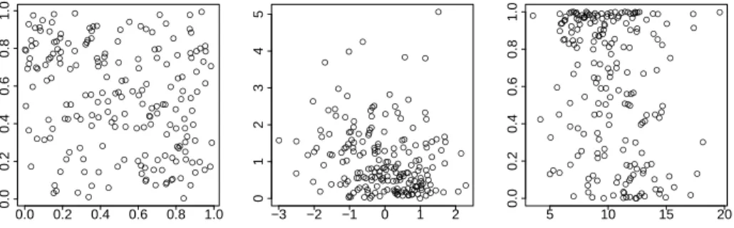
The importance of the marginal-free understanding of a dependence structure is depicted in Figure 1.1. There we see the same dependence structure for three different groups of marginal distributions.

An example of a dependence structure is positive quadrant dependence, which means that the probability that two random variables jointly exceed certain levels is greater than the probability that each exceeds the corre-sponding levels independently. It occurs to be a feature of bivariate distri-butions that does not depend on the marginal distridistri-butions. In other words, it is invariant to probability distribution transformations of the marginals.

A tool that is mainly used in dependence structure modelling and test-ing is a copula function. It is a multivariate function which links the joint distribution function with the marginal distribution functions. Although, a copula might be defined outside of the probabilistic scope, it is very useful

2 CHAPTER 1. INTRODUCTION ● ● ● ● ● ● ● ● _● ● ● ● ● ● ● ● ● ● ● ● ● ● ● ● ● ● ● ● ● ● ● ● ● ● ● ● ● ● ● ● ● ● ● ● ● ● _● ● ● ● ● ● ● ● ● ● ● ● ● ● ● ● ● ● ● ● ● ● ● ● ● ● ● ● ● ● ● ● ● ● ● ● ● ● ● ● ● ● ● ● ● ● ● ● ● ● ● ● ● ● ● ● ● ● ● ● ● ● ● ● ● ● ● ● ● ● ● ● ● ● ● ● ● ● ● ● ● ● ● ● ● ● ● ● ● ● ● ● ● ● ● ● ● ● ● ● ● ● ● ● ● ● ● ● ● ● ● ● ● ● ● ● ● ● ● ● ● ● ● ● ● ● ● ● ● ● ● ● ● ● ● ● ● ● ● ● ● ● ● ● ●_● ● ● ● ● ● ● ● ● 0.0 0.2 0.4 0.6 0.8 1.0 0.0 0.2 0.4 0.6 0.8 1.0 ● ● ●● ● ● ● ● ● ● ● ● ● ● ● ● ● ● ● ●● ● ● ● ● ● ● ● ● ● ● ● ● ● ● ● ● ● ● ● ● ● ● ● ● ● ● ● ● ● ● ● ● ● ● ● ● ● ● ● ● ● ● ● ● ● ● ● ● ● ● ● ● ● ● ● ● ● ● ● ● ● ● ● ● ● ● ● ● ● ● ● ● ● ● ● ● ● ● ● ● ● ● ● ● ● ● ● ● ● ● ● ● ● ● ● ● ● ● ● ● ● _● ● ● ● ● ● ● ● ● ● ● ● ● ● ● ● ● ● ● ● ● ● ● ● ● ● ● ● ● ● ● ● ● ● ● ● ● ● ● ● ● ● ● ● ● ● ● ● ● ● ● ● ● ● ● ● ● ● ● ● ● ● ● ● _● ● ● ● ●● ● ● ● ● ● ● ● ● −3 −2 −1 0 1 2 0 1 2 3 4 5 ● ● ● ● ● ● ● ● ● ● ● ● ● ● ● ● ● ● ● ● ● ● ● ● ● ● ● ● ● ● ● ● ● ● ● ● ● ● ● ● ● ● ● ● ● ● ● ● ● ● ● ● ● ● ● ● ● ● ● ● ● ● ● ● ● ● ● ● ● ● ● ● ● ● ● ● ● ● ● ● ● ● ● ● ● ● ● ● ● ● ● ● ● ● ●● ● ● ● ● ● ● ● ● ● ● ● ● ● ● ● ● ● ● ● ● ● ● ● ● ● ● ● ● ● ● ● ● ● ● ● ● ● ● ● ● ● ● ● ● ● ● ● ● ● ● ● ● ● ● ● ● ● ● ● _● ● ● ● ● ● ● ● ● ● ● ● ● ● ● ● ● ● ● ● ● ● ● ● ● ● ● ● ● ● ● ● ● ● ● ● ● ● ● ● ● ● ● ● ● 5 10 15 20 0.0 0.2 0.4 0.6 0.8 1.0

Figure 1.1: Samples coming from Frank(-1) copula with different marginal distri-butions.

to look at it as a multivariate distribution function with uniform margins. A copula function contains complete information about interactions between elements in a random vector. Therefore, it is essentially equivalent to the dependence structure concept. Thus, studying particular features of depen-dence structures can be accomplished by studying the corresponding features of a copula function, which is specific for a given random vector.

Developing methodology for studying dependence structures is important as the same relation patterns are of interest for various areas of science and business, which are faced with many different kinds of marginal distributions. Although studying dependence structures is broadly explored in dependence modelling, it is not as deeply investigated in testing problems.

The main contributions of this thesis consist of developing statistical tests for specific dependence structures, by exploring its copula characteri-zations. The methodology is primarily based on finite resampling from semi-parametric and non-semi-parametric constrained copula estimates. The com-prised features of dependence structures are quadrant dependence, tail mono-tonicity and stochastic monomono-tonicity. Quadrant dependence specifically com-pares the joint distribution function against the independent marginals and can be referred to as positive, negative or neither of the two. It is the weakest form of the considered dependence structures, thus contains the class of tail monotonic structures. Tail monotonicity refers to the left or the right tail and can be increasing, decreasing or neither of them. The strongest depen-dence structure considered in this thesis is stochastic monotonicity, which can be defined as increasing, decreasing or again neither of the two. Fig-ure 1.2 presents an abstract set containment of the considered characteristics of dependence structures.

3 Quadrant Dependence ∪ Tail Monotonicity ∪ Stochastic Monotonicity

Figure 1.2: Abstract inclusions of dependence structures.

Figure 1.3 depicts a part of one of the real data examples investigated in the next parts of the thesis. It presents insurance claims relating to losses in building value and the profit they generated. With the help of the developed tests in this thesis, one can answer questions such as whether these data reveal a general positive or negative relation, whether there is a monotonic pattern in the corners of the sample plot or whether there possibly is a very strong overall conditional monotonic relation between the two observed variables. The answers to these questions might be influential in the premium setting process or portfolio management for an insurance company.

We shall see that this data set reveals the positive quadrant dependence structure, according to the developed tests. Thus, the next interesting point is to check this positive dependence structure in more detail, namely by looking for existence of any positive tail monotonicity. In this case, the tests strongly reject the hypothesis that the variable ‘profits’ is left tail decreasing in the variable ‘buildings’, yet do not reject the hypothesis that the variable ‘profits’ is right tail increasing in the variable ‘buildings’. If right tail in-creasingness is not rejected, then it is interesting to check further, whether this could be caused by a certain stochastic monotonicity relation.

● ● ● ● ● ● ● ● ● ● ● ● ● ● ● ● ● ● ● ● ● ● ● ● ● ● ● ● ● ● ● ● ● ● ● ● ● ● ● ● ● ● ● ● ● ● ● ● ● ●_●● ● ● ● ● ● ● ● ● ● ● ● ● ● ● ● ● ● ● ● ●● ● ● ●●●●●●● ● ● ● ● ● ● ● ● ● ● ● ● ● ● ● ●● ● ● ● ● ● ● ● ● ● ● ●● ● ● ●●_● ● ● ●● ● ● ● ● ● ● ● ● ● ● ● ● ● ● ● ●● ● ● ● ● ● ● ● ● ● ● ●_● ● ● ● ● ● ● ● ● ● ● ● ● ● ● ● _● ● ● ● ● ● ● ● ● ● ● ● ● ● ● ● ● ● ● ● ● ● ● ● ● ● ● ● ● ● ● ● ● ● ● ● ● ● ● ● ● ● ● ● ● ●●● ● ● ●● ●●●● ● ● ● ● ● ● ● ● ● ● ● ● ● ●●●●● ● ● ● ● ● ● ● ● ● ● ● ● ● ●●● ● ● ● ●●● ● ● ● ● ● ● ● ● ● ● _●●● ●●●● ● ● ● ● ● ● ● ● ● ● ● ● ● ● ● ● ● ● ● ● ● ● ● ● ● ● ● ● ● ● ● ● ● ● ● ● ● ● ● ● ● ● ● ● ● ● ● ● ● ● ● ● ●● ● ● ● ● ● ● ● ● ● ● ● ● ● ● ● ● ● ● ● ● ● ● ● ● ● _● ● ● ● ● ●● ● ● ● ● ● ● ● ● ● ● ● ● ● _{● ●} ● ● ● ● ● ● ● ● ● ● ● ● ● ● ● ● ● ● ● _{● ●}● ● ● ● ● ● ● ● ● ● ● ● ● ● ● ● ● ● ● ●● ● ●_● ● ● ● ● ● ●● ● ● ● ● ● ● ●● ●● ● ● ● ● ● ● ● ● ● ● ● ● ● ● ● ● ● ● ● ● ● ● ● ● ● ● ● ● ● ● ● ● ● ● ● ● ● ● ● ● ● ● ● ● ● 0 1 2 3 4 5 0 1 2 3 4 5 buildings profits

4 CHAPTER 1. INTRODUCTION

The next part of the introduction contains a review of the literature con-cerning copulas in general, examples of its statistical applications in mod-elling and testing, and estimation techniques. We also briefly review the literature on the discussed dependence structures. We comment on the mod-ern applicability of these dependence structures and on existing competing testing methods. The last part of the introductory chapter will introduce mathematical definitions, properties and notations of the concepts and tools used throughout this thesis.

The following chapters describe tests for positive quadrant dependence (Chapter 2 and Chapter 3, based on papers Gijbels et al. (2010) and Gij-bels and Sznajder (2011a)), tests for tail monotonicity (Chapter 4, based on Gijbels and Sznajder (2011b)) and tests for stochastic monotonicity (Chap-ter 5, based on Gijbels and Sznajder (2011c)). Each chap(Chap-ter also includes a simulation study to investigate the power and size, the finite sample perfor-mances of the discussed tests, and to compare these with existing competing methods. Moreover, the tests are applied to a variety of real data examples.

1.1

Brief literature review

The main reference book on the copula theory used throughout this thesis is Nelsen (2006). It contains mathematical definitions and properties of a copula function, methods of construction, links to association measures and specific dependence structures. The crucial theorem on copula decomposi-tion of any multivariate distribudecomposi-tion funcdecomposi-tion is thanks to Sklar (1959).

An area where copulas are very frequently used is finance, where they mainly model the co-movement of the financial instruments with the purpose of pricing or risk management. There are several books entirely devoted to these topics, e.g., Cherubini et al. (2004), Xu (2010) and Cherubini et al. (2011) and many devote some chapters to copulas, e.g., in insurance Kaas et al. (2004) or Denuit et al. (2005).

In fact it is hard nowadays to find any domain where there is a need for dependence modelling and where copulas are not taken into account. As an example, there are references to copula usage in modern measurement and advanced psychometrics, e.g., Braeken et al. (2007) and Braeken and Tuerlinckx (2009a,b).

Because of the wide applicability of copulas in dependence modelling, the core focus in testing is being put on goodness-of-fit tests, which check the validity of the applied copula models. Among others see Genest et al. (2006), Genest and R´emillard (2008), Omelka et al. (2009), Berg (2009),

1.1. BRIEF LITERATURE REVIEW 5

Genest et al. (2009b), Genest et al. (2011) and Kojadinovic and Yan (2011). In terms of estimation of the copula function the first proposed estimator is the empirical estimator of Deheuvels (1979). The maximum likelihood estimator for a copula coming from a parametric family has been described in Genest and Rivest (1993). There has also been considerable research in semi- and non-parametric methods, e.g., Chen and Huang (2007), Omelka et al. (2009) and Genest et al. (2009a). Further developments of the copula fitting problems extended to the concept of a conditional copula are e.g., in Gijbels et al. (2011) and Veraverbeke et al. (2011) and to dynamic stochastic copulas in Hafner and Manner (2010).

The particular dependence structures studied in this thesis originate from Tukey (1958) and Lehmann (1966), and were further developed in Esary and Proschan (1972). Positive quadrant dependence as a testing problem was in-vestigated by Kochar and Gupta (1987) and Janic-Wr´oblewska et al. (2004), as test for independence against strict positive quadrant dependence. Testing for positive quadrant dependence against not positive quadrant dependence was studied by Denuit and Scaillet (2004) and Scaillet (2005).

Until now, tail monotonicity has not been an object in statistical testing. It has been however explored in the area of positive dependence orderings by Colangelo et al. (2005, 2006) and Colangelo (2008).

When first introduced by Tukey (1958), stochastic monotonicity was re-ferred to as a complete positive/negative regression feature. It is indeed a stronger relation than the nowadays widely discussed problem of (mean) regression monotonicity. In its original form, stochastic monotonicity was tested for by Lee et al. (2009), which also includes an overview of stochastic monotonicity applicability in econometrics.

6 CHAPTER 1. INTRODUCTION

1.2

Copulas

The word copula means from Latin a tie/bond, a friendly/close relation-ship, according to the William Whitaker’s Words Latin dictionary (http:

//archives.nd.edu/words.html).

1.2.1 Definition and basic properties

As already mentioned a copula function has a purely probabilistic interpre-tation, given in the following definition.

Definition 1.1. Ann-copula functionC is any continuous joint distribution function of a random vector of lengthn, where the marginal distributions are uniformly distributed on the unit intervalI= [0,1].

The tool that is mainly used in this thesis is a 2-copula, thus the term ‘copula’ will refer to that for simplicity. The following theorems are essential for the wide applicability of copulas. The proofs of all the theoretical results in this section can be found in Nelsen (2006) or in the indicated references.

Theorem 1.1 (Sklar (1959)).

• IfH is a joint distribution function with marginalsX∼F andY ∼G, then there exists a copula CX,Y (called the copula of X and Y) such that

H(x, y) =CX,Y (F(x), G(y)) ∀x, y∈R.

IfF andG are continuous, thenCX,Y is unique, else CX,Y is uniquely determined onrange(F)×range(G).

• If C is a copula and F and G are distribution functions, then the functionH=C(F, G) is a joint distribution function, with marginsF

andG.

Throughout this thesis we will always assume continuity of the marginal distribution functions.

Furthermore, as long as it is clear from the context, the notation C will be used instead ofCX,Y and the marginal distributions ofCwill be denoted asU, V ∼ U[0,1], i.e., (U, V)∼C. Moreover, we can interpret the marginals ofCX,Y asU =F(X) andV =G(Y).

1.2. COPULAS 7

Proposition 1.1. If H is a joint distribution function with marginsF and

G, then C(u, v) =H F(−1)(u), G(−1)(v) ∀(u, v)∈I2,

where F(−1) and G(−1) are pseudo-inverses of F and G respectively, e.g.,

F(−1)(t) = inf{x: F(x)≥t}.

Proposition 1.2 is often treated as a definition of a copula function. It defines the boundary (b) and measure (c) conditions of the copula function.

Proposition 1.2. For each copula C

(a) C:I×I−→I

(b) C(u,0) =C(0, v) = 0; C(u,1) =u; C(1, v) =v ∀u, v∈I

(c) C(u2, v2)−C(u1, v2)−C(u2, v1) +C(u1, v1)≥0 ∀u1≤u2, v1 ≤v2 ∈I. Condition (b) outlines the fact that any copula has uniform margins. Condition (c) is a consequence of a copula inducing a probability measureµC, building it from rectangles in the unit squareI2, i.e.,µC [u1, u2]×[v1, v2]

=

C(u2, v2)−C(u1, v2)−C(u2, v1)+C(u1, v1), which is also called theC-volume

(C-measure) of the rectangle [u1, u2]×[v1, v2].

The following theorem is important for the resampling purposes.

Theorem 1.2. If C is a copula, then

• the partial derivative ∂C_∂u exists for almost all u and for all v∈_I, and for such u and v

0≤ ∂

∂uC(u, v)≤1.

• the partial derivative ∂C_∂v exists for almost all v and for all u∈_I, and for such u and v

0≤ ∂ ∂vC(u, v)≤1. • The functions cv(u) = ∂C(u, v) ∂v and cu(v) = ∂C(u, v) ∂u

are well-defined and non-decreasing on I. Moreover, they are the con-ditional distribution functions

8 CHAPTER 1. INTRODUCTION

A very convenient property of a copula function is its behaviour under monotone transformations of the marginals. One special manifestation of Theorem 1.3 was already mentioned, namelyCX,Y =CU,V, whereU =F(X) and V =G(Y).

Theorem 1.3. If X and Y are continuous random variables with copula

CX,Y, then

• if α and β are both strictly increasing functions, then

Cα(X),β(Y)(u, v) =CX,Y(u, v),

• ifαis a strictly increasing function andβa strictly decreasing function, then

Cα(X),β(Y)(u, v) =u−CX,Y(u,1−v),

• ifαis a strictly decreasing function andβa strictly increasing function, then

C_α(X),β(Y)(u, v) =v−CX,Y(1−u, v),

• if α and β are both strictly decreasing functions, then

Cα(X),β(Y)(u, v) =u+v−1 +CX,Y(1−u,1−v).

Although it is assumed in this thesis that the distributions H,F and G

are continuous, this does not mean thatH (or C) has a density. We stress it by defining the copula decomposition components in Definition 1.2.

Definition 1.2. Any copula C can be decomposed in two parts

C(u, v) =AC(u, v) +SC(u, v), where AC(u, v) = Z u 0 Z v 0 ∂2 ∂s∂tC(s, t)dtds

is called an absolutely continuous component and

SC(u, v) =C(u, v)−AC(u, v) is called a singular component.

If C = AC, then the copula is said to be absolutely continuous and ∂2

∂s∂tC(s, t) is its joint density. If C = SC, so ∂2

∂s∂tC(s, t) = 0 almost ev-erywhere, then the copula is said to be singular.

1.2. COPULAS 9

The support of a copula, defined in Definition 1.3, is closely related to the copula decomposition. In the next section we shall see different copula examples with various decompositions and supports.

Definition 1.3. The support of the copula is the complement of the union of all open subsets of R2 with C-measure zero. If supp C = I2, then the copula is said to have full support.

The set of all copula functions is convex (Proposition 1.3) and bounded (Theorem 1.4). Via the convexity property we can obtain interesting copula examples. Bounds provide characteristic limits in the dependence structure, see Definition 1.4.

Proposition 1.3. A convex linear combination of copulas is a copula.

Theorem 1.4. If C is a copula, then

max(u+v−1,0)≤C(u, v)≤min(u, v) ∀u, v∈_I. Definition 1.4.

• W(u, v) = max(u+v−1,0)is called the Fr´echet-Hoeffding lower bound, • M(u, v) = min(u, v) is called the Fr´echet-Hoeffding upper bound. These bounds in the dependence structure intuitively indicate certain deterministic relations as specified in Proposition 1.4.

Proposition 1.4.

• Y is an increasing function of X almost surely if and only if CX,Y =

M,

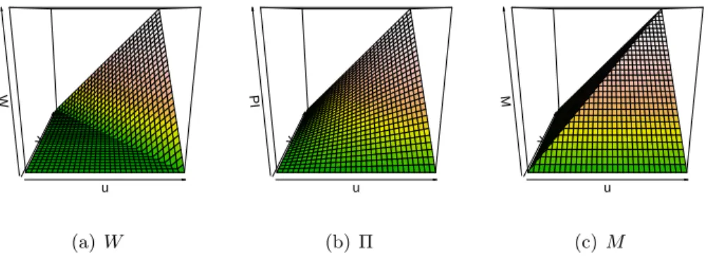
• Y is a decreasing function ofX almost surely if and only ifCX,Y =W. Furthermore, it can be shown thatW and M are valid copula functions themselves. The copulas W and M, which bind the set of all copula func-tions, are depicted in Figures 1.4 (a) and (c).

The next section gathers other copula examples used throughout this thesis.

10 CHAPTER 1. INTRODUCTION

1.2.2 Copula examples

The most characteristic copula is the independence copula, which corre-sponds to the independence of the random variables. Indeed,

P(X≤x, Y ≤y) =C F(x), G(y)=F(x)G(y) =P(X≤x)P(Y ≤y). Definition 1.5. The independence copula is denoted by Π, i.e., Π(u, v) =

uv.

In Figure 1.4 (b) we depict the independence copula Π.

u v W (a)W u v PI (b) Π u v M (c) M

Figure 1.4: CopulasW,Π andM and corresponding contour plots.

The rest of the provided examples are families of copulas. The flexibility of a copula family to model the dependence structure can be measured in different ways, yet Definition 1.6 states the nature of what one can call a broad collection of copulas.

Definition 1.6. If W,Π and M belong to a certain copula family (possibly as the limiting cases), then this copula family is called comprehensive.

A first copula family to be comprehensive is the Mardia family (Mardia (1970)), which parametrizes a convex mixture ofW, Π and M, i.e.,

CMardia =

θ2(1−θ)

2 ·W + (1−θ

2_{)·Π +}θ2(1 +θ)

2 ·M, (1.1)

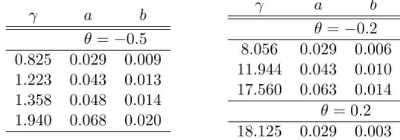
whereθ∈[−1,1]. An extension of this family is

1.2. COPULAS 11 whereωW = θ 2_(1−θ) 2 γ,ωΠ= (1−γθ 2_),ω M = θ 2_(1+θ) 2 and 0< γ≤1/θ 2_.

One of the broad collections of copulas is the class of Archimedean cop-ulas, defined in Proposition 1.5.

Proposition 1.5. If ϕis a continuous, convex and strictly decreasing func-tion from I to [0,∞] such that ϕ(1) = 0, and its pseudo-inverse is defined as ϕ[−1](t) = ϕ(−1)(t) 0≤t≤ϕ(0) 0 ϕ(0)≤t≤ ∞, then C(u, v) =ϕ[−1](ϕ(u) +ϕ(v)) is a valid copula function.

The function ϕis called a generator and ifϕ(0) =∞ it is called a strict generator.

Many parametric subclasses arose within the Archimedean copula family, e.g., • Frank ϕθ(t) =−ln e−θt−1 e−θ₋₁, θ∈R\ {0} and C−∞=W,C0= Π and C∞=M • Clayton ϕθ(t) = 1 θ t −θ₋₁ , θ∈[−1,∞)\ {0} and C−1=W,C0 = Π and C∞=M

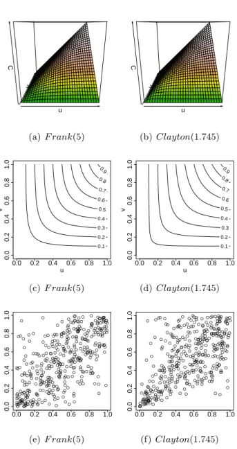
Figures 1.5 (a,b) depict exemplary copula functions coming from these two Archimedean copula families. We can see that they appear to be almost “identical” and, in general, it is extremely hard to distinguish between the copulas on the copula function level. However, if we look at the contour plots of these copula function (c,d) or samples they generate (e,f) we can see that these two copula distributions are very different.

12 CHAPTER 1. INTRODUCTION u v C (a)F rank(5) u v C (b) Clayton(1.745) u v 0.1 0.2 0.3 0.4 0.5 0.6 0.7 0.8 0.9 0.0 0.2 0.4 0.6 0.8 1.0 0.0 0.2 0.4 0.6 0.8 1.0 (c) F rank(5) u v 0.1 0.2 0.3 0.4 0.5 0.6 0.7 0.8 0.9 0.0 0.2 0.4 0.6 0.8 1.0 0.0 0.2 0.4 0.6 0.8 1.0 (d) Clayton(1.745) ● ● ● ● ● ● ● ● ● ● ● ● ● ● ● ● ● ● ● ● ● ● ● ● ● ● ● ● ● ● ● ● ● ● ● ● ● ● ● ● ● ● ● ● ● ● ● ● ● ● ● ● ● ● ● ● ● ● ● ● ● ● ● ● ● ● ● ● ● ● ● ● ● ● ● ● ● ● ● ● ● ● ● ● ● ● ● ● ● ● ● ● ● ● ● ● ● ● ● ● ● ● ● ● ● ● ● ● ● ● ● ● ● ● ● ● ● ● ● ● ● ● ● ● ● ● ● ● ● ● ● ● ● ● ● ● ● ● ●_● ● ● ● ● ● ● ● ● ● ● ● ● ● _● ● ● ● ● ● ● ● ● ● ● ● ● ● ● ● ● ● ● ● ● ● ● ● ● ● ● ● ● ● ● ● ● ● ● ● ● ● ● ● ● ● ● ● ● ● ● ● ● ● ● ● ● ● ● ● ● ● ● ● ● ● ● ● ● ● ● ● ● ● ● ● ● ● ● ● ● ● ● ● ● ● ● ● ● ● ● ● ● ● ● ● ● ● ● ● ● ● ● ● ● ● ● ● ● ● ● ● ● ● ● ● ● ● ● ● ● ● ● ● ● ● ● ● ● ● ● ● ● ● ●●● ● ● ● ● ● ● ● ● ● ● ● ● ● ● ● ● ● ● ● ● ● ● ● ● ● ● ● ● ● ● ● ● ● ● ● ● ● ● ● ● ● ● ● ● ● ● ● ● ● ● ● ● ● ● ● ● ● ● ● ● ● ● ● ● ● ● ● ● ● ● ● ● ● ● ● ● ● ● ● ● ● ● ● ● ● ● ● ● ● ● ● ● ● ● ● ● ● ● ● ● ● ● ● ● ● ● ● ● ● ● ● ● ● ● 0.0 0.2 0.4 0.6 0.8 1.0 0.0 0.2 0.4 0.6 0.8 1.0 (e) F rank(5) ● ● ● ● ● ● ● ● ● ● ● ● ● ● ● ● ● ● ● ● ● ● ● ● ● ● ● ● ● ● ● ● ● ● ● ● ● ● ● ● ● ● ● ● ● ● ● ● ● ● ● ● ● ● ● ● ● ● ● ● ● ● ● ● ● ●● ● ● ● ● ● ● ● ● ● ● ● ● ● ● ● ● ● ● ● ● ● ● ● ● ● ● ● ● ● ● ● ● ● ● ● ● ● ● ● ● ● ● ● ● ● ● ● ● ● ● ● ● ● ● ● ● ● ● ● ● ● ● ● ● ● ● ● ● ● ● ● ● ● ● ● ● ● ● ● ● ● ● ● ● ● ● ● ● ● ● ● ● ● ● ● ● ● ● ● ● ● ● ● ● ● ● ● ● ● ● ● ● ● ● ● ● ● ● ● ● ● ● ● ● ● ● ● ● ● ● ● ● ● ● ● ● ● ● ● ● ● ● ● ● ● ● ● ● ● ● ● ● ● ●● ● ● ● ● ● ● ● ● ● ● ● ● ● ● ● ● ● ● ● ● ● ● ● ● ● ● ● ● ● ● ● ● ● ● ● ● ● ● ● ● ● ● ● ● ● ● ● ● ● ● ● ● ● ● ● ● ● ● ● ● ● ● ● ● ● ● ● ● ● ● ● ● ● ● ● ● ● ● ● ● ● ● ● ● ● ● ● ● ● ● ● ● ● ● ● ● ● ● ● ● ● ● ● ● ● ● ● ● ● ● ● ● ● ● ● ● ● ● ● ● ● ● ● ● ● _● ● ● ● ● ● ● ● ● ● ● ● ● ● ● ● ● ● ● ● ● ● ● ● ● ● ● ● ● ● ● ● ● ● ● ● ● ● ● ● ● ● ● ● ● ● ● ● ● ● ● ● ● 0.0 0.2 0.4 0.6 0.8 1.0 0.0 0.2 0.4 0.6 0.8 1.0 (f) Clayton(1.745)

Figure 1.5: Two examples of Archimedean copula functions together with 400

1.2. COPULAS 13

The last class of copulas to describe in this introduction is a copula obtained by specifying a cross sectional function. Specifically, it is a class of copulas with quadratic sections, which is based on Proposition 1.6.

Proposition 1.6. If ψ is a function on the unit interval such that • ψ is absolutely continuous on I,

• |ψ0(v)| ≤1 almost everywhere on I, • |ψ(v)| ≤min(v,1−v) ∀v∈_I, then

C(u, v) =uv+ψ(v)u(1−u) is a valid copula function.

In the next section we recall the main copula estimation method used in the rest of the thesis.

1.2.3 Nonparametric estimation of a copula and resampling

Based on Proposition 1.1 a natural estimator forC can be built on an em-pirical version of the distribution functions H, F and G. Throughout this thesis we shall use the asymptotically equivalent version of such estimator coming from Deheuvels (1979) and we will refer to this one as the empirical copula estimator, i.e., having a random sample (Xi, Yi) n_i=1 from (X, Y) then Cn(u, v) = 1 n n X i=1 I{Uˆi≤u, Vˆi ≤v}, (1.3) where ˆUi = _n+1n Fn(Xi) and ˆVi = _nn₊₁Gn(Yi), with Fn and Gn the empirical distribution function estimators ofX andY. The values ˆUi and ˆVi are often called the pseudo-observations in the literature.

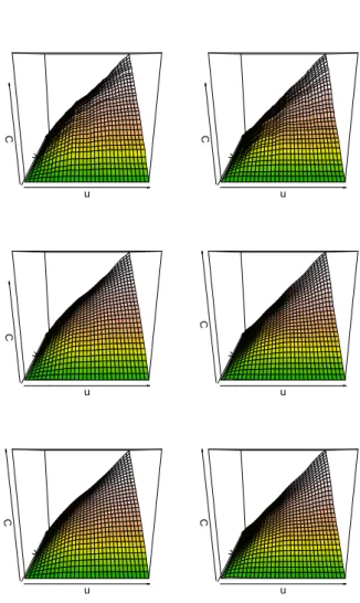
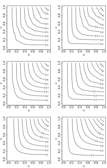
In Chapter 2 we shall be working with other recently developed non-parametric copula estimators, specifically the kernel local linear estimator of Chen and Huang (2007), the kernel mirror-reflection estimator of Gijbels and Mielniczuk (1990) and their shrunken versions introduced in Omelka et al. (2009). Figure 1.6 gathers the copula estimates corresponding to the samples in Figures 1.5 (c) and (d). As underlined earlier, it is hard to visibly distinguish even very distinctive copula functions, therefore Figure 1.7 presents the corresponding contour plots.

14 CHAPTER 1. INTRODUCTION u v C u v C u v C u v C u v C u v C

Figure 1.6: Copula estimates based on the samples in Figure 1.5 (c) (left column) and (d) (right column) for different non-parametric estimators: empirical (top row), kernel local linear shrunken (middle row) and kernel mirror-reflection (bottom row).

1.2. COPULAS 15 u v 0.1 0.2 0.3 0.4 0.5 0.6 0.7 0.8 0.9 0.0 0.2 0.4 0.6 0.8 1.0 0.0 0.2 0.4 0.6 0.8 1.0 u v 0.1 0.2 0.3 0.4 0.5 0.6 0.7 0.8 0.9 0.0 0.2 0.4 0.6 0.8 1.0 0.0 0.2 0.4 0.6 0.8 1.0 u v 0.1 0.2 0.3 0.4 0.5 0.6 0.7 0.8 0.9 0.0 0.2 0.4 0.6 0.8 1.0 0.0 0.2 0.4 0.6 0.8 1.0 u v 0.1 0.2 0.3 0.4 0.5 0.6 0.7 0.8 0.9 0.0 0.2 0.4 0.6 0.8 1.0 0.0 0.2 0.4 0.6 0.8 1.0 u v 0.1 0.2 0.3 0.4 0.5 0.6 0.7 0.8 0.0 0.2 0.4 0.6 0.8 1.0 0.0 0.2 0.4 0.6 0.8 1.0 u v 0.1 0.2 0.3 0.4 0.5 0.6 0.7 0.8 0.0 0.2 0.4 0.6 0.8 1.0 0.0 0.2 0.4 0.6 0.8 1.0

16 CHAPTER 1. INTRODUCTION

It is to be noted that none of these estimators is a valid copula function. In particular, the empirical copula estimator clearly does not fulfill condi-tion (b) in Proposicondi-tion 1.2 as it is a jump funccondi-tion by construccondi-tion. All of these estimators are however consistent estimators. Constructing a copula estimator which is a copula itself is not an easy task.

According to Theorem 1.2 we can describe a general resampling process from a given copula C as follows.

Algorithm 1.1.

1. Draw two observations u, t from the uniform distribution on the unit interval

2. and compute v=c−1_u (t).

Now, (u, v) is an observation from the distributionC and we can repeat the process to obtain a sample of observations of a given size.

Having a copula estimator which is itself a copula is essential in resam-pling. It is possible to approximately resample from the smoothed versions of copula estimators, but it is not enough for the proposed testing proce-dures. What is needed is a flexible way to resample from a constrained copula estimator. By constrained we mean a copula estimator which (at least ap-proximately) satisfies certain copula shape structure conditions specified in the next section. There is no clear way to modify existing copula estimation methods to obtain a copula estimator constrained to an arbitrary shape. Therefore, a new generic method is proposed in the thesis.

The main concept relies on smoothing the initial discrete constrained copula estimator. Let us specify a grid of points {(ui, vj)}m_i,j+1₌₀ on the unit square and compute the corresponding constrained copula values ci,j for

i, j = 0, . . . , m+ 1. Then we can apply any smoothing technique to obtain the first order partial derivate estimate based on{ci,j}m_i,j+1₌₀. In this thesis we focus on the local linear smoothing methodology, see e.g., Wand and Jones (1995) and Fan and Gijbels (1996). Specifically, we approximatecu(v) of the constrained copula estimate in the following way.

cu,n(v) = [0,1,0](X0W X)−1X0W Y, (1.4) where Y =    c0,0 .. . cm+1,m+1   , X =    1 u0−u v0−v .. . 1 um+1−u vm+1−v   ,

1.2. COPULAS 17 W =    kh1(u0−u)kh2(v0−v) 0 . .. 0 kh1(um+1−u)kh2(vm+1−v)    and khl(x) = 1 hl k x hl l= 1,2,

where k is a kernel function (a symmetric probability density function),

hl>0, l= 1,2, are the bandwidth parameters andX0 is transpose ofX. To make sure thatcu,n(v) is a valid (univariate) distribution function on the unit interval we monotonize it and fit the range properly.

The monotonization technique used throughout the thesis is based on an appealing monotonic rearrangement technique, see e.g., Lieb and Loss (2001).

Definition 1.7. Let the functionξ denote the increasing rearrangement op-erator defined as

ξ(f)(t) =

Z

A

I(f(x)≤t)dx ∀t∈B, (1.5)

on the space of univariate real-valued bounded functionsf:A→B withA a bounded set.

The idea behind the rearrangement operator is to construct a non-decreas-ing “inverse” of a given function and apply the operator twice to receive a non-decreasing “version” of the original function. As a result, we obtain a function with appealing properties.

Proposition 1.7. If ξ is the increasing rearrangement operator of Defini-tion 1.7, then

(a) ξ is uniquely defined,

(b) (ξ◦ξ)(f) is a non-decreasing function on A, (c) if f is non-decreasing, then (ξ◦ξ)(f)≡f, (d) for any non-decreasing functiong:A→B

||(ξ◦ξ)(f)−g||_Lp(A)≤ ||f−g||_Lp(A),

where || · ||_Lp(A) denotes the norm of p-integrable functions (on the set

18 CHAPTER 1. INTRODUCTION

The next section defines the specific dependence structures introduced in the beginning of the chapter.

1.3

Dependence structures

The specific dependence structures that are studied in this thesis are quad-rant dependence, tail monotonicity and stochastic monotonicity.

Quadrant dependence is the most general kind of dependence and is closely connected to the common association measures.

1.3.1 Association measures

The relation commonly used in statistics to describe the position of points in a two-dimensional space can be expressed as a relation of the components.

Definition 1.8. If(xi, yi),(xj, yj)are two observations from a vector(X, Y) of continuous random variables, then they are concordant if {xi < xj and

yi < yj} or {xi > xj and yi > yj}, and they are discordant if{xi < xj and

yi> yj} or {xi > xj andyi < yj}.

In other words the observations are concordant if (xi−xj)(yi−yj)>0 and are discordant if (xi−xj)(yi−yj)<0.

This ordering leads to an aggregate measure of concordance.

Definition 1.9. If {(x1, y1), . . . ,(xn, yn)} is a random sample of n obser-vations from the vector (X, Y) of continuous random variables and c is the number of concordant pairs and d is a number of discordant pairs, then the Kendall’s tau for the sample is

τn= c−d c+d = c−d n 2 .

It is clearly a sample probability of concordance minus sample probability of discordance. On the population level Kendall’s tau is defined analogously.

Definition 1.10. Kendall’s tau for the random vector(X, Y) is defined as

τX,Y =P (X1−X2)(Y1−Y2)>0

−_P (X1−X2)(Y1−Y2)<0

,

where (X1, Y1) and (X2, Y2) are independent copies of (X, Y).

It occurs that Kendall’s tau does not depend on the marginals and is purely a feature of a dependence structure, thus can be expressed in terms of copulas.

1.3. DEPENDENCE STRUCTURES 19

Theorem 1.5. If X andY are continuous random variables with copula C, then

τX,Y =τC = 4

Z Z

I2

C(u, v)dC(u, v)−1 = 4E C(U, V)−1. (1.6) For the Archimedean copula family the general expression (1.6) can be rewritten in the following way.

Proposition 1.8. If C is an Archimedean copula with generator ϕ, then

τC = 1 + 4 Z 1 0 ϕ(t) ϕ0_(t)dt= 1−4 Z ∞ 0 u d duϕ [−1] (u) 2 du.

Another commonly used dependence measure is Spearman’s rho, which again measures certain concordance discrepancies.

Definition 1.11. Spearman’s rho for the random vector (X, Y) is defined as ρX,Y = 3 P (X1−X2)(Y1−Y3)>0 −_P (X1−X2)(Y1−Y3)<0 ,

where (X1, Y1), (X2, Y2) and (X3, Y3) are independent copies of (X, Y).

In other words, Spearman’s rho measures the concordance and discor-dance for (X1, Y1) and (X2, Y3), where X2 and Y3 are independent, so their

copula is Π. This leads to the following theorem.

Theorem 1.6. If X andY are continuous random variables with copula C, then ρX,Y =ρC = 12 Z Z I2 uvdC(u, v)−3 = 12 Z Z I2 C(u, v)dudv−3.

Note thatρC can be rewritten as

ρC = 12E(U, V)−3 = E(U, V)−1₄ 1 12 = pE(U, V)−EUEV Var(U)pVar(V)

and hence Spearman’s rho is identical to the Pearson’s correlation coefficient for random variablesU =F(X) and V =G(Y).

Furthermore, Spearman’s rho is a “scaled” volume under the graph of the copula, but as

ρC = 12 Z Z I2 C(u, v)dudv−3 = 12 Z Z I2 C(u, v)−uv dudv, (1.7)

20 CHAPTER 1. INTRODUCTION

it can also be interpreted as proportional to the signed volume between the graphs of the copula C and the product copula Π. Thus ρC is a measure of “average distance” between the joint distributions ofX and Y (as repre-sented byC) and independence (as represented by Π).

This difference between a given copula C and the independence copula Π is the essence of quadrant dependence.

1.3.2 Quadrant dependence

Definition 1.12. Random variables X and Y are positively quadrant de-pendent (P QD(X, Y)) if for all x, y∈_R

P(X≤x, Y ≤y)≥P(X ≤x)P(Y ≤y), or equivalently

P(X > x, Y > y)≥P(X > x)P(Y > y). (1.8)

By analogy we can define negative quadrant dependence (N QD(X, Y)). In other words, P QD(X, Y) holds if

H(x, y)≥F(x)G(y) ∀x, y∈_R or equivalently

C(u, v)≥uv ∀u, v∈_I. (1.9)

This is thus a feature of the dependence structure regardless of the marginal distributions.

We can now rephrase (1.7) and say that Spearman’s rho is a measure of the “average” quadrant dependence of a copulaC.

Quadrant dependence is also easily tractable after the monotonic marginal transformations.

Proposition 1.9. LetXandY be positively quadrant dependentP QD(X, Y). If α is a strictly increasing function, and β1 and β2 are strictly decreasing

functions, then

• β1(X),α(Y) are negative quadrant dependentN QD β1(X), α(Y)

, • α(X), β2(Y) are negative quadrant dependentN QD α(X), β2(Y)

, • β1(X),β2(Y) are positive quadrant dependent P QD β1(X), β2(Y)

1.3. DEPENDENCE STRUCTURES 21

Going back to the given copula examples, we can see that the indepen-dence copula can be seen as a boundary point in the sets of both PQD and NQD copulas. This important fact will be explored for testing in the next chapters. As for the other copula examples, we can see that the Mardia families are neither PQD nor NQD, and the quadratic section copula family is PQD if and only if ψ is a negative function and NQD if it is non-positive. Positive quadrant dependence in the Archimedean copula class is described in the following proposition.

Proposition 1.10. If an Archimedean copula C has a strict generator ϕ, then it is PQD if and only if −lnϕ(−1) is subadditive on (0,∞), i.e.,

lnϕ(−1)(x+y)≥lnϕ(−1)(x) + lnϕ(−1)(y) ∀x, y∈[0,∞).

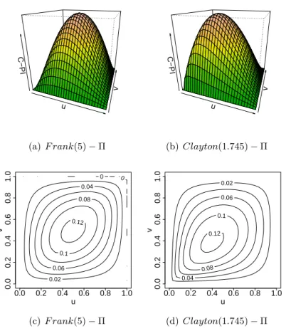
In case of the two introduced subclasses of Archimedean copulas, the Frank and Clayton copula families, the PQD feature is preserved for the non-negative parameter values and NQD for the non-positive ones. Fig-ure 1.8 depicts examples of Frank and Clayton copula functions minus the independence copula function Π.

Reformulation of Definition 1.12 evolves in the next studied characteristic of the dependence structure, namely tail monotonicity. We say thatX and

Y are positive quadrant dependent if

P(Y ≤y|X≤x)≥P(Y ≤y|X≤ ∞). (1.10) Intuitively this means that for any fixed y the conditional probability of

Y ≤y given X ≤ x is greater than the same probability for x = ∞. One way to assure that is to ask this probability to be a decreasing function ofx

for any fixedy.

1.3.3 Tail monotonicity

Definition 1.13.

• Y is left tail decreasing in X (LT D(Y|X)) if

P(Y ≤y|X≤x) is a non-increasing function of x for all y. • Y is right tail increasing in X (RT I(Y|X)) if

22 CHAPTER 1. INTRODUCTION u v C−PI (a)F rank(5)−Π u v C−PI (b)Clayton(1.745)−Π u v 0 0 0.02 0.04 0.06 0.08 0.1 0.12 0.0 0.2 0.4 0.6 0.8 1.0 0.0 0.2 0.4 0.6 0.8 1.0 (c)F rank(5)−Π u v 0.02 0.04 0.06 0.08 0.1 0.12 0.0 0.2 0.4 0.6 0.8 1.0 0.0 0.2 0.4 0.6 0.8 1.0 (d)Clayton(1.745)−Π

Figure 1.8: Difference between Frank and Clayton copula functions and the inde-pendence copula function and the corresponding contour plots.

By analogy we define left tail increasing and right tail decreasing relations, and also the analogous X|Y relations.

It follows from (1.10) that Y being left tail decreasing in X implies X

and Y being positively quadrant dependent, yet even more holds.

Proposition 1.11.

• LT D(Y|X) or LT D(X|Y) implies P QD(X, Y) • RT I(Y|X) or RT I(X|Y) implies P QD(X, Y). Note that the opposite does not necessarily hold.

1.3. DEPENDENCE STRUCTURES 23

The above tail monotonic properties can also be expressed in terms of copulas. The following expressions are of crucial use in this thesis.

Proposition 1.12.

• LT D(Y|X) if and only if for everyv C(u, v)

u is non-increasing in u (1.11)

• RT I(Y|X) if and only if for every v

1−u−v+C(u, v)

1−u is non-decreasing in u,

or equivalently, if

v−C(u, v)

1−u in non-increasing in u.

Referring back to the copula examples, we can see that the independence copula fulfills all of the tail monotonic structure conditions, thus can be again treated as a boundary point of each set of copulas. The Mardia families have none of the tail monotonic properties and the considered two subclasses of Archimedean copula families are LTD and RTI for non-negative parameter values, and LTI and RTD for non-positive ones. Furthermore, there is a general condition for the Archimedean copulas to be LTD.

Proposition 1.13. If an Archimedean copula C has a strict generator ϕ, then it is LTD if and only ifϕ(−1) is completely monotone on(0,∞), i.e., it is continuous on(0,∞) and

(−1)k d k

dtkϕ

(−1)_{(t)≥0 ∀t∈(0,∞) and k = 0,1, . . . .}

Moreover, as the Archimedean copula functions are all symmetric in their variables, the tail monotonicity properties are the same forY|X and X|Y.

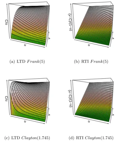
Figure 1.9 presents the functions from Proposition 1.12 C/u and (v−

C)/(1−u) reflecting the LTD (Figures 1.9 (a) and (c)) and RTI (Figures 1.9 (b) and (d)) properties of the two examples of Archimedean copula functions. The cubic section copula family is in general not easily described in terms of tail monotonicity, yet it is easy to see that we haveLT D(V|U) and

RT I(V|U) if ψ is a non-negative function.

The last considered feature of dependence structure comes from even further narrowing the relation in (1.10).

24 CHAPTER 1. INTRODUCTION u v C/u (a) LTDF rank(5) u v (v−C)/(1−u) (b) RTIF rank(5) u v C/u (c) LTDClayton(1.745) u v (v−C)/(1−u) (d) RTIClayton(1.745) Figure 1.9: Frank and Clayton functions reflecting LTD and RTI.

1.3.4 Stochastic monotonicity

Definition 1.14. Y is stochastically increasing inX(SI(Y|X)) if for every

y

P(Y > y|X =x) is a non-decreasing function of x. AnalogouslySD(Y|X) is defined.

Again, note that Y being stochastically increasing inX implies Y being left tail decreasing inX and generalizes to the following.

Proposition 1.14. SI(Y|X) implies LT D(Y|X) and RT I(Y|X).

In terms of copulas stochastic monotonicity can be expressed for example in the following way.

1.3. DEPENDENCE STRUCTURES 25

Proposition 1.15. SI(Y|X) if and only if for everyv,C(u, v) is a concave function ofu.

For the discussed copula examples the conclusions are the same as for the tail monotonicity case and the general condition for the Archimedean copulas is the following.

Proposition 1.16. If an Archimedean copula C has a strict generator ϕ

andϕ−1 is differentiable, then it is SI if and only if ln−dϕ_dt−1(t) is convex on(0,∞).

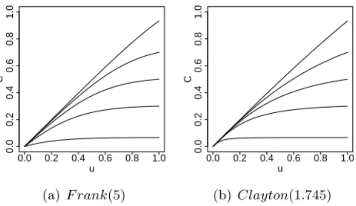
From Figure 1.8, where we plot C −Π, we can deduce that the given examples of Archimedean copulas are concave functions ofufor everyv. For convenience we also plot several sections of the same copulas in Figure 1.10.

0.0 0.2 0.4 0.6 0.8 1.0 0.0 0.2 0.4 0.6 0.8 1.0 u C (a)F rank(5) 0.0 0.2 0.4 0.6 0.8 1.0 0.0 0.2 0.4 0.6 0.8 1.0 u C (b) Clayton(1.745)

Figure 1.10: Copula sectionsC(u, v), for several fixed values of v, for Frank and Clayton copulas.

Before moving to the next chapter let us refer back to Figure 1.5, where we have seen samples for Frank and Clayton copula family members. The parameters of each were chosen such as to provide the same theoretical value of Spearman’s rho equal to 0.64. These samples already look clearly very different from each other. In Figure 1.1 it was only one copula sample transformed with a variety of marginal distributions. For all three joint distributions Spearman’s rho equals 0.16. From both figures and examples it is clear that it is hardly possible to “guess” from a scatterplot of the data anything about characteristics of the underlying dependence structure. Therefore, statistical tests that test for a specific dependence structure are needed. This thesis contributes largely to this topic.

Chapter 2

Positive quadrant

dependence tests for copulas

2.1

Introduction

This chapter is based on Gijbels et al. (2010) and develops tests for positive quadrant dependence.

A concept that is symmetric to PQD is the concept of NQD, which swaps the inequality in the definition of PQD. The relation between both concepts can be seen in terms of monotonic transformations. Applying in-creasing functions to X and Y does not change the copula, thus neither their quadrant dependence. However, if an increasing function is applied to one random variable and a decreasing function to the other random variable, then the quadrant dependence of the transformed couple of random variables is changed, see also Proposition 1.9.

Positive quadrant dependence might be a very realistic assumption in many situations. Think of, for example, life expectancies of men and women in various countries. One would expect that a higher life expectancy for men in one country goes along with a higher life expectancy for women in that country. Examples of positive quadrant dependence are ample in particular in insurance and finance. For a discussion about PQD in finance and actuarial sciences see Janic-Wr´oblewska et al. (2004) and Denuit and Scaillet (2004) and references therein. The knowledge about PQD or NQD of random variables is important for statistical inference. Indeed, if it is reasonable to assume, for example, positive quadrant dependence then such prior knowledge should be exploited in the statistical inference.

Janic-Wr´oblewska et al. (2004) and Denuit and Scaillet (2004) also

28 CHAPTER 2. POSITIVE QUADRANT DEPENDENCE TESTS FOR COPULAS

vestigate testing problems related to this type of dependence structure. In Janic-Wr´oblewska et al. (2004) rank tests are introduced for testing inde-pendence against positive quadrant deinde-pendence. Testing for indeinde-pendence against strict PQD was dealt with in Kochar and Gupta (1987). Denuit and Scaillet (2004) test for PQD against non-PQD and construct tests based on a distance concept considering the PQD definitions of both (1.8) and (1.9) using empirical cumulative distribution function estimators.

In this chapter we are concerned with testing the null hypothesis of posi-tive quadrant dependence versus not posiposi-tive quadrant dependence, focusing as such on finding out whether a PQD assumption is justified. Starting from the PQD characteristic of a copula function given in (1.9), the basic idea of the testing procedures here is to investigate a distance between a non-parametric estimate of the unknown copula and the independence copula function. We consider various non-parametric estimators of a copula func-tion along with three funcfunc-tional distances.

Testing for positive quadrant dependence was also studied in Scaillet (2005). In that paper the author constructs a Kolmogorov-Smirnov type of test based on the empirical copula estimator relying on the asymptotic distribution of the empirical process. Statistical inference is conducted by using a simulation-based multiplier method and a bootstrap method. The present paper contributes further on this testing problem in various aspects. Firstly, testing procedures based on other distance measures such as Cram´ er-von Mises and Anderson-Darling distance measures (see e.g., Anderson and Darling (1954)) should be studied, since they might reveal different power properties, see also Omelka et al. (2009). Secondly, in recent years other competitive and improved non-parametric estimators of a copula have been introduced and studied and it is worth to investigate how these estimators perform when used in testing procedures. In our study we consider the empirical copula estimator of Deheuvels (1979), kernel type estimators such as the integrated version of the density Mirror Reflection estimator (see Gijbels and Mielniczuk (1990)) and the Local Linear estimator (see Chen and Huang (2007)), as well as recent extensions (improvements) of these two kernel estimators introduced and studied in Omelka et al. (2009). Thirdly, relying on asymptotic theory is not always the best option, since the rate of convergence might require rather large samples before good finite sample behaviour is obtained. We therefore opt for a different approach here, and make use of the independence copula as a reference case included in the null hypothesis. Admittedly this approach also has drawbacks but, as will be seen, these are overruled by the advantages in power performance.

2.2. NONPARAMETRIC COPULA ESTIMATION AND TEST STATISTICS 29

This chapter is organized as follows. In Section 2.2, we briefly discuss the various non-parametric copula estimators and the different test statistics, and establish consistency of these testing procedures. The proofs of these results are given in Section 2.6. Section 2.3 contains a simulation study illustrating the finite sample behaviour of the tests. In Section 2.4 we apply these procedures on real data examples. We conclude in Section 2.5 with some further discussions on the research topic.

2.2

Nonparametric copula estimation and test

sta-tistics

Copula estimation is closely related to the estimation of a cumulative distri-bution function with the main difference that no data from (F(X), G(Y)) are observed. Referring to the definition of a copula, an estimation procedure can be divided into two levels, estimation of the marginals and estimation of their joint distribution. If on both levels parametric assumptions are made, then maximum likelihood methods can be applied. However, it is com-mon to make parametric assumptions on the joint level combined with non-parametric estimation of marginals, resulting in popular semi-non-parametric models. For this usage, there are many well described copula families differ-ing in the number of parameters and characteristics (see e.g., Nelsen (2006)). In this chapter we are interested in a fully non-parametric approach, and in particular in recently developed estimation procedures described in Omelka et al. (2009). A basic idea behind this and previous estimation methods is to transform the observed data by a monotonic transformation, specifically by the empirical marginal distribution functions, and then to estimate the joint distribution function based on these pseudo-observations. As such we can unify random vectors, which have the same copula, regardless of their marginal distributions.

Suppose we have a sample (X1, Y1), . . . ,(Xn, Yn)∼iidH =C(F, G). The pseudo-observations as already defined are

ˆ Ui= n n+ 1Fn(Xi), Vˆi= n n+ 1Gn(Yi),

whereFn and Gn are the empirical distributions. The modification _nn₊₁ to the empirical distribution simply pulls the pseudo-observations a bit more away from one (see Genest et al. (1995)). By doing so potential difficulties arising at boundaries can be reduced. The pseudo-observations are then treated as a sample from the random vector (F(X), G(Y)) ∼ C and the

30 CHAPTER 2. POSITIVE QUADRANT DEPENDENCE TESTS FOR COPULAS

copula C can be estimated non-parametrically as a bivariate distribution on the unit square. However, because of the unit square domain there are boundary issues arising in the estimation task. Therefore, in our testing procedure, we investigate along with the empirical estimator, the kernel estimators of Chen and Huang (2007) and Gijbels and Mielniczuk (1990) together with their “shrunken” modifications proposed by Omelka et al. (2009) for better consistency results.

In summary our study involves the following copula estimators: • Empirical copula estimator (Deheuvels (1979))

Cn(u, v) = 1 n n X i=1 I{Uˆi≤u,Vˆi≤v},

whereI{A}denotes the indicator function of A.

• Kernel Local Linear estimator (Chen and Huang (2007)) Denoted by ˆCLL n : ˆ C_nLL(u, v) = 1 n n X i=1 Ku,hn u−Uˆi hn ! Kv,hn v−Vˆi hn ! ,

where hn is a smoothing parameter and Ku,hn(x) =

Rx

−∞ku,hn(t)dt is

the integral of the modified kernel

ku,h(x) = k(x) (a2(u, h)−a1(u, h)x) a0(u, h)a2(u, h)−a21(u, h) I{u −1 h < x < u h}, where a`(u, h) = Z u<sub>h</sub> u−1 h t`k(t)dt for`= 0,1,2

and k is a symmetric kernel function that is bounded on the unit interval, e.g., the Epanechnikov kernelk(x) = 0.75(1−x2)I{|x| ≤1}. • Kernel Local Linear Shrunken estimator (Omelka et al. (2009))

Denoted by ˆCLLS n : ˆ C_nLLS(u, v) = 1 n n X i=1 Ku,hn u−Uˆi b(u)hn ! Kv,hn v−Vˆi b(v)hn ! , whereb(w) =pmin(w,1−w).

2.2. NONPARAMETRIC COPULA ESTIMATION AND TEST STATISTICS 31

• Kernel Mirror-Reflection estimator (Gijbels and Mielniczuk (1990)) Denoted by ˆC_nMR: ˆ C_nMR(u, v) = 1 n n X i=1 9 X `=1 " K u− ˆ U<sub>i</sub>(`) hn ! −K − ˆ U_i(`) hn !# · " K v−Vˆ (`) i hn ! −K −Vˆ (`) i hn !# , where {( ˆU<sub>i</sub>(`),Vˆ_i(l)), i= 1, . . . , n, `= 1, . . . ,9}= ={(±Uˆi,±Vˆi),(±Uˆi,2−Vˆi),(2−Uˆi,±Vˆi),(2−Uˆi,2−Vˆi), i= 1, . . . , n}, and K(x) =Rx

−∞k(t)dt is the integral of the considered kernelk.

• Kernel Mirror-Reflection Shrunken estimator (Omelka et al. (2009)) Denoted by ˆC_nMRS: ˆ C_nMRS(u, v) = 1 n n X i=1 9 X `=1 " K u− ˆ U<sub>i</sub>(`) b(u)hn ! −K − ˆ U_i(`) b(u)hn !# · " K v−Vˆ (`) i b(v)hn ! −K −Vˆ (`) i b(v)hn !# .

It should be mentioned that in Chen and Huang (2007) the pseudo-observations are obtained via kernel methods. The authors showed however that strong undersmoothing is needed in this step, and hence we here decided directly for a rank estimation, which coincides with the limiting case that the smoothing parameter tends to zero.

The test statistics for testing for positive quadrant dependence are based on distances between the estimated copula and the independence copula. The distances measure the violation part of the copula estimator with the positive quadrant dependence hypothesis under the null. We focus on mea-sures based on L∞ and L2 distances. Denote by ˆCn the estimated copula distribution function. We then consider the following statistics

• Kolmogorov-Smirnov

S_nKS =√n sup u,v∈[0,1]

(uv−Cˆ_n(u, v))+,

32 CHAPTER 2. POSITIVE QUADRANT DEPENDENCE TESTS FOR COPULAS

• Cram´er-von Mises

S_nCvM=n Z I2 (uv−Cˆ_n(u, v))2₊dCˆ_n(u, v). • Anderson-Darling S_nAD=n Z I2 (uv−Cˆ_n(u, v))2₊ uv(1−u)(1−v)dCˆn(u, v).

Note that the correction factor (uv(1−u)(1−v))−1in the Anderson-Darling distance puts more attention to the boundaries of a copula. This weight factor is in fact the asymptotic variance of the empirical copula estimator (based on pseudo-observations) when the true underlying copula is the inde-pendence copula. Such a weighting factor is also appealing from an intuitive point of view since the closer one gets to the boundaries the smaller the absolute differences between the copulas are. In addition crucial differences between copulas (and therefore between dependency structures) are often hidden close to the boundaries.

With a specified copula estimator and a functional distance, and an i.i.d. sample (X1, Y1), . . . ,(Xn, Yn) from a joint distribution with underlying cop-ulaC, we can build a test statisticSn to test the null hypothesis of positive quadrant dependence

H0 : ∀u, v∈[0,1] C(u, v)≥uv

against the negation of this

H1 : ∃u, v∈[0,1] C(u, v)< uv.

The distribution ofSnunder the null hypothesis is unknown and there are various options to tackle this problem. A first option is to rely on asymptotic results for the copula estimator at hand. For all copula estimators mentioned above weak convergence results are available. Possible drawbacks of this ap-proach are that the asymptotics might kick in only for rather large sample sizes, that the test statistics are non-trivial functionals of the copula esti-mator, and that it typically requires estimation of partial derivatives of the copula function, resulting in a rather complex estimation procedure. A sec-ond approach is to use resampling methods to mimic the distribution ofSn under the null hypothesis. The multiplier and bootstrap methods of Scaillet (2005) follow these approaches. A potential problem with these two meth-ods is that the resampling should in fact be done under the null hypothesis, which cannot be guaranteed.