Network intrusion detection using genetic programming.

Network Intrusion Detection using Genetic

Programming

by

Tatenda H Chareka

Submitted in fulfilment of the academic requirements of

Master of Science

in the

School of Mathematics, Statistics, and Computer Science

College of Agriculture, Engineering and Science

University of KwaZulu-Natal

Pietermaritzburg

South Africa

November 2018

As the candidate’s supervisor, I have/have not approved this thesis/dissertation for submission Signed: ____________________________

Name: Prof. Nelishia Pillay Date: ____________________________

i

PREFACE

The research contained in this dissertation was completed by the candidate while based in

the Discipline of Computer Science, School of Mathematics, Statistics and Computer Science

of the College of Agriculture, Engineering and Science, University of KwaZulu-Natal,

Pietermaritzburg, South Africa. National Research Funding financially supported the research.

The contents of this work have not been submitted in any form to another university and,

except where the work of others is acknowledged in the text, the results reported are due to

investigations by the candidate.

_________________________ _________________________ Signed: Professor Nelishia Pillay Signed: Tatenda Chareka Date: 20 November 2018 Date: 28 November 2018

ii

DECLARATION 1: PLAGIARISM

I, Tatenda Chareka (student number: 211506553), declare that:

(i) the research reported in this dissertation, except where otherwise indicated or acknowledged, is my original work;

(ii) this dissertation has not been submitted in full or in part for any degree or examination to any other university;

(iii) this dissertation does not contain other persons’ data, pictures, graphs or other information, unless specifically acknowledged as being sourced from other persons;

(iv) this dissertation does not contain other persons’ writing, unless specifically acknowledged as being sourced from other researchers. Where other written sources have been quoted, then: a) their words have been re-written but the general information attributed to them has

been referenced;

b) where their exact words have been used, their writing has been placed inside quotation marks, and referenced;

(v) where I have used material for which publications followed, I have indicated in detail my role in the work;

(vi) this dissertation is primarily a collection of material, prepared by myself, published as journal articles or presented as a poster and oral presentations at conferences. In some cases, additional material has been included;

(vii) this dissertation does not contain text, graphics or tables copied and pasted from the Internet, unless specifically acknowledged, and the source being detailed in the dissertation and in the References sections.

_____________________________________________ Signed: Tatenda Chareka

iii

DECLARATION 2: PUBLICATIONS

DETAILS OF CONTRIBUTION TO PUBLICATIONS that form part and/or include research presented in this thesis

Publication 1:

CHAREKA, T. & PILLAY, N. A study of fitness functions for data classification using grammatical evolution. Pattern Recognition Association of South Africa and Robotics and Mechatronics International Conference (PRASA-RobMech), 2016, 2016. IEEE, 1-4.

iv

Abstract

Network intrusion detection is a real-world problem that involves detecting intrusions on a computer network. Detecting whether a network connection is intrusive or non-intrusive is essentially a binary classification problem. However, the type of intrusive connections can be categorised into a number of network attack classes and the task of associating an intrusion to a particular network type is multiclass classification.

A number of artificial intelligence techniques have been used for network intrusion detection including Evolutionary Algorithms. This thesis investigates the application of evolutionary algorithms namely, Genetic Programming (GP), Grammatical Evolution (GE) and Multi-Expression Programming (MEP) in the network intrusion detection domain. Grammatical evolution and multi-expression programming are considered to be variants of GP. In this thesis, a comparison of the effectiveness of classifiers evolved by the three EAs within the network intrusion detection domain is performed. The comparison is performed on the publicly available KDD99 dataset. Furthermore, the effectiveness of a number of fitness functions is evaluated.

From the results obtained, standard genetic programming performs better than grammatical evolution and multi-expression programming. The findings indicate that binary classifiers evolved using standard genetic programming outperformed classifiers evolved using grammatical evolution and multi-expression programming. For evolving multiclass classifiers different fitness functions used produced classifiers with different characteristics resulting in some classifiers achieving higher detection rates for specific network intrusion attacks as compared to other intrusion attacks. The findings indicate that classifiers evolved using multi-expression programming and genetic programming achieved high detection rates as compared to classifiers evolved using grammatical evolution.

v

Acknowledgements

I would like to thank the National Research Foundation (NRF) for the financial assistance. The opinions raised and conclusions reached, are those of the author and are not attributed to the NRF. The Centre of High-Performance Computing (CHPC) for granting access to their resources.

I would like to thank my supervisor, Professor Nelishia Pillay for her constant support and guidance throughout the compilation of this thesis. I would also like to thank my family members, friends and colleagues for their continuous support and motivation.

vi

Contents

PREFACE ... i

DECLARATION 1: PLAGIARISM ... ii

DECLARATION 2: PUBLICATIONS ... iii

Abstract ... iv

Acknowledgements ... v

Contents ... vi

List of Figures ... xii

List of Tables ... xiv

List of Algorithms ... xvi

List of Abbreviations ... xvii

1

Introduction ... 1

Purpose of the Study ... 1

Aims and Objectives ... 1

Contributions ... 2

Dissertation Layout ... 2

2

Genetic Programming ... 5

Introduction ... 5

Introduction to Genetic Programming ... 6

Overview of the GP Algorithm ... 6

Representation ... 7

2.4.1

Tree Based GP ... 7

2.4.2

Function Set ... 7

2.4.3

Terminal Set ... 8

Initial Population Generation ... 8

2.5.1

Full Method ... 9

2.5.2

Grow Method ... 9

2.5.3

Ramped Half and Half Method ... 10

Evaluation ... 10

vii

2.6.2

Fitness Functions ... 11

Selection Methods ... 12

2.7.1

Tournament Selection ... 12

Genetic Operators ... 13

2.8.1

Reproduction ... 13

2.8.2

Mutation ... 14

2.8.3

Crossover ... 14

GP Control Models ... 15

2.9.1

Generational Model ... 16

2.9.2

Steady State Model ... 16

Termination ... 17

Introns and Bloat ... 17

Modularisation ... 18

Strengths and Weaknesses of GP ... 18

2.13.1

Strengths ... 18

2.13.2

Weaknesses ... 18

Introduction to Grammatical Evolution ... 19

Overview of the Generational GE Algorithm ... 19

Representation ... 20

2.16.1

BNF Grammar ... 20

2.16.2

Mapping Process ... 21

Initial Population Generation and Evaluation ... 23

Genetic Operators ... 23

2.18.1

Crossover ... 24

2.18.2

Mutation ... 25

Introns and Bloat ... 26

Strengths and Weakness of GE ... 27

2.20.1

Strengths ... 27

2.20.2

Weaknesses ... 27

Introduction to Multi-Expression Programming ... 28

Overview of the Steady State MEP Algorithm ... 28

Representation ... 29

viii

Genetic Operators ... 31

2.25.1

Crossover ... 31

2.25.2

Mutation ... 33

Introns and Modularisation ... 34

Strengths and Weakness of MEP ... 34

2.27.1

Strengths ... 34

2.27.2

Weaknesses ... 34

Chapter Summary ... 34

3

Network Intrusion Detection ... 36

Introduction ... 36

Network Intrusion Detection ... 37

Datasets for Network Intrusion Detection ... 38

3.3.1

DARPA 1998 and 1999 ... 39

3.3.2

KDD Cup 99 ... 40

3.3.3

NSL-KDD dataset ... 41

3.3.4

Network Attack Categories ... 41

Performance Measures ... 42

3.4.1

Confusion matrix ... 43

3.4.2

Accuracy and False Positive Rate ... 43

3.4.3

Sensitivity and Specificity ... 44

3.4.4

Precision and F-measure ... 44

3.4.5

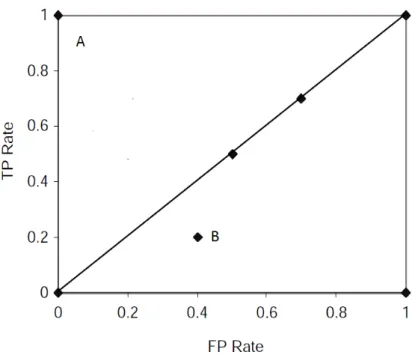
Receiver operating characteristics ... 44

Feature Selection ... 45

Previous Work on Network Intrusion Detection ... 46

3.6.1

Evolutionary Algorithms ... 46

3.6.2

Neural Networks ... 46

3.6.3

Bayesian Networks ... 47

3.6.4

Decision Trees ... 47

Chapter Summary ... 48

4

GP and Network Intrusion Detection ... 49

Introduction ... 49

Using genetic programming for network intrusion detection ... 49

ix

4.3.1

Genetic Programming ... 50

4.3.2

Grammatical Evolution ... 52

4.3.3

Linear Genetic Programming ... 53

Multiclass Classification for NID using GP ... 53

4.4.1

Genetic Programming ... 53

4.4.2

Grammatical Evolution ... 54

4.4.3

Multi-expression Programming ... 54

4.4.4

Linear genetic programming ... 54

Strengths and Weaknesses of GP in NID ... 55

4.5.1

Strengths ... 55

4.5.2

Weaknesses ... 55

Analysis of genetic programming in network intrusion detection ... 55

Chapter Summary ... 57

5

Methodology ... 58

Introduction ... 58

Research Methodology ... 58

5.2.1

Aims and Objectives ... 58

Proof by Demonstration Methodology ... 59

5.3.1

Evaluation of approach ... 60

5.3.2

Refinement of approach ... 60

5.3.3

Termination Criterion ... 61

Statistical Tests ... 61

5.4.1

Statistical Testing ... 61

Dataset ... 62

5.5.1

Dataset description ... 62

5.5.2

Dataset Pre-processing ... 62

5.5.3

Binary classification dataset ... 63

5.5.4

Multi-class classification dataset ... 64

Distributed Architecture for Proposed Approaches ... 64

Technical Specifications ... 65

Chapter Summary ... 65

6

Genetic Programming for Network Intrusion Detection ... 66

x

GP Algorithm ... 66

Representation and initial population generation ... 67

Evaluation ... 68

Selection Method and Genetic Operators ... 71

Parameters ... 73

Chapter Summary ... 74

7

Grammatical Evolution for Network Intrusion Detection ... 75

Introduction ... 75

Representation ... 75

Initial Population Generation and Evaluation ... 77

Selection Method and Genetic Operators ... 78

Parameters ... 79

Chapter Summary ... 80

8

Multi-Expression Programming for Network Intrusion Detection ... 81

Introduction ... 81

MEP Algorithm ... 81

Representation ... 82

Initial Population Generation and Evaluation ... 83

Selection Method and Genetic Operators ... 83

Parameters ... 85

Chapter Summary ... 86

9

Results and Discussion ... 87

Introduction ... 87

Grammatical Evolution ... 88

9.2.1

Binary Classification ... 88

9.2.2

Multi-class classification ... 88

9.2.3

Analysis of multi-class classification for GE approach ... 93

Multi-Expression Programming ... 94

9.3.1

Binary Classification ... 94

9.3.2

Multi-class classification ... 94

9.3.3

Analysis of multi-class classification for MEP approach ... 99

Genetic Programming ... 100

xi

9.4.2

Multi-class classification ... 101

9.4.3

Analysis of multi-class classification for the GP approach ... 105

Comparison of GP, GE and MEP ... 106

9.5.1

Binary classification ... 106

9.5.2

Multi-class classification ... 108

Comparison with state of the art ... 109

9.6.1

Binary Classification ... 109

9.6.2

Multi-class classification ... 110

Chapter Summary ... 111

10

Conclusion and Future Work ... 113

Introduction ... 113

Objectives and Conclusion ... 113

Bibliography ... 116

A.

User Manual ... 124

Program requirements ... 124

Initialising the Program ... 124

Overview of the program ... 124

xii

List of Figures

Figure 2.1: Tree depth ... 8

Figure 2.2: Full and Grow Tree Generation... 9

Figure 2.3: Ramped half-and-half ... 10

Figure 2.4: Mutation operation ... 14

Figure 2.5: Crossover operation ... 15

Figure 2.6: GE fixed length one-point crossover ... 24

Figure 2.7: GE two-point crossover ... 24

Figure 2.8: Homologous Crossover ... 25

Figure 2.9: Mutation Operator Variations ... 26

Figure 2.10: MEP chromosome genes represented as trees ... 31

Figure 2.11: MEP one-point crossover ... 32

Figure 2.12: MEP two-point crossover ... 32

Figure 2.13: MEP uniform crossover... 33

Figure 2.14: MEP Mutation ... 33

Figure 3.1: The NID process ... 37

Figure 3.2: DARPA, KDD99 and NSL-KDD relation. ... 39

Figure 3.3: ROC graph ... 45

Figure 5.1: Binary classification distribution... 64

Figure 5.2: Multi-class Classification distribution... 64

Figure 6.1: Example of an individual ... 68

xiii

Figure 6.3: GP Crossover ... 72

Figure 6.4: GP Mutation ... 73

Figure 7.1: Binary to denary conversion... 77

Figure 7.2: GE Individual ... 77

Figure 7.3: GE uniform crossover ... 78

Figure 8.1: MEP Individual ... 83

Figure 8.2: MEP Uniform Crossover ... 85

Figure 9.1: GE comparison of fitness function performance ... 93

Figure 9.2: MEP comparison of fitness function performance ... 100

Figure 9.3: GP comparison of fitness function performance ... 105

Figure 9.4: Binary classification comparison ... 106

Figure 9.5: Multi-class classification comparison ... 108

Figure A.1: Network Intrusion Detection System Main Menu ... 124

Figure A.2: Train and Test using NID System ... 125

Figure A.3: End of run Message ... 126

Figure A.4: Selecting best classifier ... 126

xiv

List of Tables

Table 2.1: Fitness Cases ... 11

Table 2.2: The number of choices for each production rule ... 22

Table 3.1: KDD Cup 99 Sample Distribution ... 40

Table 3.2: KDD Cup Class distribution ... 41

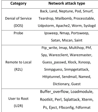
Table 3.3: Network intrusion detection categories ... 42

Table 3.4: Binary confusion Matrix ... 43

Table 5.1: Z-hypothesis test table ... 61

Table 5.2: NSL-KDD sample distribution ... 62

Table 5.3: Data transformation ... 63

Table 6.1: Function descriptions ... 68

Table 6.2: Confusion Matrix ... 71

Table 6.3: GP Parameters for binary classifiers... 73

Table 6.4: GP Parameters for multi-class classifiers ... 74

Table 7.1: GE Parameters for binary classification ... 79

Table 7.2: GE Parameters for multi-class classification ... 80

Table 8.1: MEP Parameters for binary classification ... 86

Table 8.2: MEP Parameters for multi-class classification ... 86

Table 9.1: Grammatical Evolution binary classification results ... 88

Table 9.2: Grammatical Evolution accuracy multi-classification results ... 89

Table 9.3: Grammatical Evolution MCC multi-classification results ... 90

xv

Table 9.5: Grammatical Evolution TPR multi-classification results ... 91

Table 9.6: Grammatical Evolution precision multi-classification results ... 92

Table 9.7: Grammatical Evolution FPR multi-classification results ... 93

Table 9.8: Multi-Expression programming binary classification results ... 94

Table 9.9: MEP accuracy multi-classification results ... 95

Table 9.10: MEP Matthews’s coefficient correlation multi-classification results ... 96

Table 9.11: MEP f-score multi-classification results ... 96

Table 9.12: MEP true positive rate multi-classification results ... 97

Table 9.13: MEP precision multi-classification results ... 98

Table 9.14: MEP false positive rate multi-classification results ... 98

Table 9.15: Genetic programming binary classification results ... 100

Table 9.16: GP accuracy multi-classification results ... 102

Table 9.17: GP Matthews’s coefficient correlation multi-classification results ... 102

Table 9.18: GP f-score multi-classification results ... 103

Table 9.19: GP true positive rate multi-classification results ... 104

Table 9.20: GP precision multi-classification results ... 104

Table 9.21: GP false positive rate multi-classification results ... 105

Table 9.22: Statistical test results for binary classification ... 107

Table 9.23: Statistical test results for multi-class classification ... 109

Table 9.24: State of the art for binary classification ... 110

xvi

List of Algorithms

Algorithm 2.1: Generational GP ... 16

Algorithm 2.2: Steady State GP ... 17

Algorithm 2.3: Generational GE Algorithm ... 19

Algorithm 2.4: Steady-State MEP Algorithm ... 28

Algorithm 5.1: Proof by demonstration ... 59

Algorithm 6.1: GP Algorithm ... 67

Algorithm 6.2: Tournament selection ... 71

xvii

List of Abbreviations

Abbreviation

Definition

NID Network Intrusion Detection

GP Genetic Programming

MEP Multi-Expression Programming GE Grammatical Evolution EA Evolutionary Algorithms

GA Genetic Algorithm

ADF Automatically Defined Functions IDS Intrusion Detection System NIDS Network Intrusion Detection System DARPA Defence Advanced Research Projects Agents AFRL Air Force Research Laboratory TCP Transmission Control Protocol

DOS Denial of Service

R2L Remote to Local L2R Local to Root TP True Positive TN True Negative FP False Positive FN False Negative Acc Accuracy

FPR False Positive rate

TPR True Positive Rate

TNR True Negative Rate

PPV Precision

ROC Receiver Operating Characteristics SVM Support Vector Machine RBF Radial Basis Function SOM Self-Organization Map WEKA Waikato Environment for Knowledge Analysis

xviii

UADR Unknown attack detection rate LERAD Learning Rules for Anomaly Detection LBNL Lawrence Berkeley National Laboratory MANET Mobile Ad hoc Networks LGP Linear Genetic Programming

DT Decision Trees

1

1

Introduction

Purpose of the Study

Network intrusion detection is a real-world problem that involves detecting intrusions on a computer network. Detecting whether a network connection is intrusive or non-intrusive is essentially a binary classification problem. However, the type of intrusive connections can be categorized into a number of network attack classes and the task of associating an intrusion to a particular network type is multiclass classification.

Various techniques have been used for network intrusion detection including Naive Bayes classification, decision tree classification, neural networks and evolutionary algorithms, amongst others. Evolutionary algorithms such as genetic programming and its variants have been widely applied for network intrusion detection but a comparison of the performance of each variant within network intrusion detection has not been addressed. This dissertation also seeks to conduct a thorough analysis of related literature on the application of genetic programming and its variants for network intrusion detection.

Aims and Objectives

The primary objective of this dissertation is to develop, and evaluate the classification performance of genetic programming and variants of genetic programming, grammatical evolution and multi-expression programming for network intrusion detection. The objectives of this dissertation are:

Objective 1: Development and evaluation of applying grammatical evolution (GE) for generating intrusion detection classifiers

To propose and implement binary and multi-class classifiers for network intrusion detection (NID) and evaluate the performance of applying GE for evolving NID classifiers.

2

Objective 2: Development and evaluation of applying Multi-expression programming (MEP) for generating binary and multi-class classifiers for network intrusion detection.

To propose, implement and evaluate the performance of evolving classifiers using MEP for intrusion detection.

Objective 3: Development and evaluation of applying genetic programming (GP) for generating binary and multiclass classifiers for network intrusion detection.

Investigate the performance of binary and multi-class classifiers evolved using GP and compare the performance of the classifiers to state-of-the-art approaches.

Objective 4: Investigate the effectiveness of fitness functions for multi-class network intrusion detection

To investigate the effects of applying different fitness functions for the generation of intrusion detection classifiers and if there a correlation between the detection rate achieved by the classifier and the fitness function used.

Objective 5: Comparative analysis of GE, MEP and GP for network intrusion detection.

A comparative analysis of binary and class classifiers evolved using grammatical evolution, multi-expression programming and genetic programming will be performed to evaluate which of the approaches generates the most effective classifiers.

Contributions

This dissertation makes the following contributions:

• Design and evaluation of generating effective classifiers using genetic programming, grammatical evolution and multi-expression programming.

• Comparative analysis of the effects of fitness functions when evolving binary and multi-class intrusion detection classifiers.

• Comparative analysis of the performance of intrusion detection classifiers generated using different variants of genetic programming.

Dissertation Layout

This section provides a summary of the chapters in this dissertation.

3

This chapter provides an introduction to genetic programming and its variants, grammatical evolution and multi-expression programming. A thorough description of each process within the variants is provided.

Chapter 3 – Network intrusion detection

Network intrusion detection (NID) is introduced in this chapter. The datasets and performance measures used within NID are also described as well as current and previous research work done within the network intrusion detection domain.

Chapter 4 – Genetic Programming and Network Intrusion Detection

This chapter reviews studies conducted within the network intrusion detection domain as well as an analysis of using genetic programming and its variants for network intrusion detection.

Chapter 5 – Methodology

The methodology used to achieve the aims and objectives outlined in Section 1.2 is discussed in this chapter. The statistical tests used to evaluate the performance of algorithms is provided in this chapter as well as a detailed description of the datasets used for this thesis.

Chapter 6 – Genetic Programming for Network Intrusion Detection

This chapter details the proposed genetic programming approach for binary and multi-class network intrusion detection.

Chapter 7 – Grammatical Evolution for Network Intrusion Detection

The grammatical evolution approach for binary and multi-class network intrusion detection is presented in this chapter.

Chapter 8 – Multi-Expression Programming for Network Intrusion Detection

The multi-expression programming approach used for binary and multi-class classification is presented in this chapter.

Chapter 9 – Results and Discussion

This chapter presents the results of each of the proposed approaches discussed from chapter six to eight. A comparison of the performance between each of the genetic programming variants is performed.

4

Chapter 10 – Conclusion and Future Work

This chapter summarizes the findings presented in this thesis and a conclusion to each of the objectives outlined in Chapter 1. The chapter also discusses future work which will be investigated.

5

2

Genetic Programming

Introduction

This chapter introduces genetic programming and its variants as well as provides details of the different aspects of the algorithm.

Sections 2.2 introduces genetic programming, followed by an overview of genetic programming in section 2.3. Representation in genetic programming is discussed in section 2.4, initial population generation methods are discussed in section 2.5. Each individual within a genetic programming population is evaluated for performance and these evaluation methods are discussed in section 2.6. Selection methods are provided in section 2.7 and genetic operators are discussed in section 2.8. Control models are discussed in section 2.9 and termination criteria used in GP are described in section 2.10. Introns and bloat are discussed in section 2.11, details of modularisation are provided in section 2.12 and the strengths and weaknesses of genetic programming are provided in section 2.13.

Section 2.14 introduces grammatical evolution, one of the variants of genetic programming. Section 2.15 provides an overview of grammatical evolution, followed by the representation in section 2.16. Initial population generation in grammatical evolution is discussed in section 2.17 and the genetic operators used in grammatical evolution are described in section 2.18. Introns and bloat in the context of grammatical evolution is discussed in section 2.19 followed by an overview of the strengths and weakness of grammatical evolution in section 2.20.

Multi-expression programming is introduced in section 2.21. Multi-expression programming is one of the variants of genetic programming. The overview of multi-expression programming is provided in section 2.22, followed by the representation in section 2.23. Section 2.24 discusses the initial population generation for multi-expression programming and genetic operators are discussed in section 2.25. Introns and modularisation within multi-expression programming is discussed in section

6

2.26 followed by the strengths and weaknesses of multi-expression programming in section 2.27. Section 2.28 presents a summary of the critical aspects of genetic programming and its variants.

Introduction to Genetic Programming

Evolutionary algorithms (EA) are a class of optimization algorithms from artificial intelligence which take an analogy from evolution to solve computer science problems. The user defines a goal in the form of a quality criterion and the EA uses the defined goal to measure and compare solutions through a number of iterations until an optimal or near optimal solution is found [3]. Solutions are found in the search space. The search space is a search area which contains potential solutions to a problem. Most evolutionary algorithms adopt processes such as reproduction, selection and mutation from Darwin’s theory of natural selection and evolution in order to efficiently find solutions within the search space [81]. The theory of natural selection states that individuals with certain characteristics (stored in the genes) are more likely to survive and replicate their characteristics to the offspring and gradually improve the characteristics of the population created [25]. Different EAs differ in the way in which solutions are represented and the way in which new solutions are derived from existing solutions. A genetic algorithm (GA) is an evolutionary population-based algorithm that was inspired by John Holland in the early 1970s to model Darwin’s theory of natural selection. A GA evolves a population of individuals towards better solutions. Each individual within the population is encoded as a string which represents a potential solution to a given problem. The GA searches for solutions to problems within the solution space [53, 81].

Genetic programming (GP) pioneered by Koza [40], is a problem solving EA in which programs are evolved to find solutions to problems. GP conducts search for a solution program to a problem in the program space. GP mimics the theory of natural selection and it is closely related to GAs. GP searches a program space and a GA searches a solution space resulting in the structure of the representations being different. GP is stochastic in nature; it is not guaranteed to find the global optimum, but a good enough solution defined by the researcher.

Overview of the GP Algorithm

A suitable representation is initially required before the GP algorithm is executed. The GP algorithm begins by generating a population of individuals made up from a combination of functions and terminals suitable for the domain. The population of individuals initially created is termed the initial population. Each individual in the initial population is assigned a value to determine how fit the individual is. The assigned value is termed as the fitness. Based on the fitness of the individual, the

7

algorithm can terminate execution. If a solution is found in the initial population, the algorithm terminates and returns the solution individual.

If a solution is not found in the initial population, the individuals go through transformations using genetic operators to create better individuals. Each transformation creates a generation. A generation is a population of individuals which are created using genetic operators. A selection method is used to select individuals from the population. Genetic operators are applied to the individuals selected. Individuals created from the application of genetic operators are referred to as offspring. After each generation, each offspring created is evaluated for quality. The generation of offspring iteratively continues until a solution is found or termination criterion is reached. The iterative process can either replace the whole population of individuals or specific individuals with a low fitness. The process from initial population generation, genetic operator applications, generations until a termination criterion is met is defined as a run. Each of the fundamental aspects of a GP run are discussed further in the following sections.

Representation

Elements of the GP population are programs, commonly represented as parse trees [74]. Other program representations include linear and graph representations [3]. A number of factors are considered when selecting the representation to use, these factors include efficiency, ease of implementation and information to be represented by the individuals [74]. A parse tree is comprised of elements of the function and terminal sets. The elements of the function and terminal sets are collectively called primitives. Genetic programming using a parse tree representation is also known as tree-based GP. Tree-based GP, functions and terminals are discussed below.

2.4.1 Tree Based GP

Each individual is represented as a parse tree for tree-based GP. Koza [40] represented programs in LISP (S-expression) which is equivalent to a parse tree representing a computer program. Pre-order notation is usually used to express parse trees for easy interpretation. Each parse tree is made up of one or several nodes. The first node within the parse tree is referred to as the root and the nodes that are found at the bottom of the parse tree are the leaves.

2.4.2 Function Set

The function set contains domain dependent functions. Mathematical functions, conditional statements, logical operators are examples of some of the functions. User defined functions can also be included in the function set. Each function has an arity. Arity is the number of arguments which a function takes [3].

8

2.4.3 Terminal Set

The terminal set is comprised of variables that make up the trees used to solve the GP problem. The variables can be of type string, real, integer or character. Constants such as ephemeral constants can be included in the trees used to solve the problem. Random ephemeral constants are values that fall within a specific range and remain unchanged during the entire duration of the run. For example, a random ephemeral constant with a range of integer values [1, 10] can be used, during a GP run if the ephemeral constant is selected, a random integer will be selected from the range [1, 10] and remain fixed for the duration of the GP run. Multiple ephemeral constants with different values can be used and the range is problem dependent. Elements of the terminal set have an arity of zero [3].

Initial Population Generation

The initial population is made up of randomly created individuals. Three methods exist for the generation of the initial population namely full, grow, and ramped half and half [40]. The generation of each individual begins by randomly selecting a function from the function set to represent the root node of the individual. The root node of the tree is selected from the function set in order to eliminate the creation of trivial trees (trees with a terminal element as the root node). Based on the arity of the root node selected, children are randomly chosen from the function and terminal sets and these are expanded iteratively in a depth first manner until a complete tree is created. The maximum depth of a tree is the distance from the root node to the bottom-most leaf node. In Figure 2.1, the root node of the individual is located at depth 1, whilst the child nodes of the root are located at depth 2 and the maximum depth of the tree is depth 4. The maximum depth of a tree is specified when creating the initial population in order to limit the size of the tree during initial population generation.

depth 1

depth 2

depth 3

depth 4 Maximum depth = 4

9

If the search space is not sufficiently represented during initial population generation, it may lead to premature convergence to a local optimum of the GP algorithm. The search space has to be sufficiently represented in order to increase the chances of finding a global optimum. The number of individuals created is controlled by the population size which is specified as one of the parameters of a GP algorithm.

2.5.1 Full Method

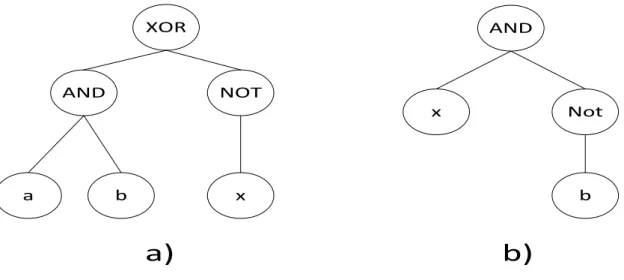
The full method creates individuals which have a balanced tree. Balanced trees have all the leaf nodes at the same depth. The internal nodes for the trees are randomly selected from the function set only until the maximum tree depth is reached. At the maximum tree depth, only nodes from the terminal set are selected. Figure 2.2a illustrates a tree created using the full method. Trees created using full might not have the same number of nodes due to different functions possessing different arity values. The method promotes less variety within the population due to the similarity in the structure of the individuals created. AND Not x b XOR AND NOT x b a

a)

b)

Figure 2.2: Tree individuals created using a) Full method and b) Grow method

2.5.2 Grow Method

The grow method creates individuals with irregular shapes and sizes [40]. The root of the individual is randomly selected from the function set. The rest of the nodes are randomly selected from either the function or terminal set until the tree depth limit is reached. Once the tree depth limit is reached only elements from the terminal set are selected. Figure 2.2b illustrates an individual created by the grow method. The grow method promotes greater variety within the population due to individuals possessing different shapes and sizes.

10

2.5.3 Ramped Half and Half Method

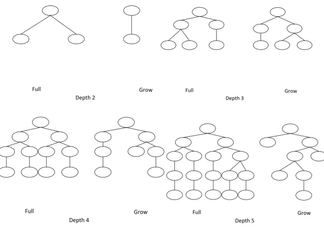
The ramped half and half method combine the full and grow methods discussed above. Half the population is created using the full method and the other half of the population is created using the grow method. An equal number of trees of each depth are also created. Koza [40] introduced this method of generation to provide a wide variety of trees created with different sizes and shapes.

For example, given a population size of 16 with a maximum tree depth of 5, at each tree depth half the population is created using the full method and the other half using the grow method. This means that at depth of 2, two individuals are created using the grow method and another two using the full method, at depth 3, two individuals using grow and two individuals using full, this continues until the maximum tree depth of 5 is reached. Figure 2.3 illustrates individuals created using the ramped half-and-half method.

Full Grow

Depth 2 Full Depth 3 Grow

Full Grow

Depth 4 Full Depth 5 Grow

Figure 2.3: Ramped half-and-half

Evaluation

Each individual within a population is evaluated in terms of how well it solves a problem. Fitness provides a measure to the GP algorithm regarding which individuals should be given a higher

11

probability of being removed from the population as well as which individuals should be allowed to reproduce and recombine with other individuals within the population [3]. Evaluating the fitness of an individual is problem dependent and literature provides a vast amount of methods to use. Fitness cases and fitness functions are used to calculate fitness.

2.6.1 Fitness Cases

Programs within the population are executed over a set of different training cases. These training cases are referred to as fitness cases. Fitness cases are input-output pairs which describe the output to be produced by individuals given particular input values [3]. The success of a GP algorithm is to an extent dependent on the choice of fitness cases. Fitness cases should provide a good ratio of representing the problem domain to ensure generalization over the solutions produced by a GP run. The fitness of an individual is a function of the output produced by the individual and the target value for each fitness case. Table 2.1 provides an illustration of fitness cases.

Input Values Output X Y 4 10 116 5 7 74 6 3 45 7 9 130

Table 2.1: Fitness Cases

2.6.2 Fitness Functions

A numerical measure of how well an individual represents a solution is calculated using a fitness function. They can be used to evaluate how well an individual expresses the fitness cases [3]. The fitness function is a fitness measure that is used to compare different individuals within the population with respect to how far or close an individual is from the desired output. Different fitness functions are used for different problem domains. Fitness functions play an important role in driving the GP algorithm towards the global optimum and they should be designed carefully in order to prevent them from driving the algorithm towards local optima [42]. Raw fitness is one of the simplest and most commonly used fitness measures. It measures how promising an individual is at solving the problem. The error function is another commonly used fitness function. In some domains a high raw fitness represents a better individual whereas in some domains, it represents a weak individual [40]. Another fitness measure commonly used is the number of hits. The number of hits is the number of fitness cases for which the value produced by an individual is the same for each fitness case. It is used to

12

determine whether a solution has been found. For example, if a GP individual represents an expression

𝑥𝑥2_{+ 𝑦𝑦}2 _{based on the fitness cases provided in Table 2.1, the number of hits would be 4 signifying a}

solution to the problem since there are four fitness cases. The greater the number of hits, the better the individual. In certain problem domains, the raw fitness is equivalent to the hits ratio.

Fitness functions have either a single objective or multiple objectives where two or more different measures are combined to solve a problem. These fitness functions are referred to as multi-objective fitness functions [3].

Selection Methods

Selection methods are methods used to select individuals responsible for offspring generation. The selected individuals are referred to as parents. Selection methods use fitness measures to select parents. Commonly employed selection methods are tournament selection and fitness-proportionate selection [40, 74]. Other selection methods used include truncation, ranking, linear and exponential selection [3].

Selection methods offer different effects on evolution and offspring generation. One of the effects is referred to as selection pressure. Selection pressure is the degree to which fitter individuals are favoured. Algorithms with high selection pressure favour fitter individuals as compared to algorithms with lower selection pressure. Selection pressure also controls the convergence rate of a GP approach; very high selection pressure may lead to premature convergence whilst a low selection pressure leads to a slower rate of convergence [52].

2.7.1 Tournament Selection

A random number of individuals are selected from the population to perform in a tournament. Comparison of each of the individuals within the tournament using the fitness value is performed. Based on the fitness the best individual is returned. The number of individuals randomly selected is referred to as the tournament size. A small tournament size promotes lower selection pressure and a high tournament size promotes higher selection pressure [3]. Tournament selection is commonly used within GP.

Tournament selection can also be applied inversely. Inverse tournament selection is applied in the same manner with tournament selection but instead of returning the best individual from the tournament, the worst individual is returned. Inverse tournament selection is used within the steady state GP control method discussed later in this chapter.

13

Genetic Operators

Genetic operators are search operators used to create individuals within a population. Genetic operators alter existing individuals in the hope of generating better offspring which solve the problem [40]. The offspring created are of different sizes and shapes as compared to their parents. Genetic operators are used to explore different areas of the program space through exploitation and exploration. Exploration is used to visit entirely new regions of the program space and genetic operators which favour exploration are termed as global search operators. Exploitation on the other hand is used to visit regions of the program space within the neighbourhood of previously visited areas. Local search operators is the term associated with genetic operators which make use of exploitation [14]. A good ratio between exploitation and exploration needs to be maintained to ensure the search converges to a global optimum. During the evolution process, exploration is recommended at the early stages rather than exploitation to ensure the best area of the program space is explored and as the evolution progresses exploitation is more favoured to ensure that the algorithm converges. Various genetic operators have been used during the evolutionary process of GP. The three most commonly used genetic operators, reproduction, mutation and crossover, are discussed in detail below. Other genetic operators include permutation, decimation, encapsulation, hoist, create [40]. The choice of genetic operators to use is usually probabilistic and the probability of application is referred to as operator application rates [74]. The operator rates are used to determine the number of offspring created by each of the genetic operators. The rates can be represented as percentage values, for example, a population of 200 individuals and a 50%, 30% and 20% application rate for crossover, mutation and reproduction respectively results in 100 individuals being created using crossover, 60 offspring created using mutation and 40 individuals created using the reproduction operator. Operator application rates are specified at the beginning of a GP run.

Genetic operators can create very large offspring and pruning can be used to ensure that the individuals do not grow beyond a certain size. This is achieved by replacing all the function nodes at a specified tree depth (offspring depth) with randomly selected terminal nodes.

Some genetic operators have been criticized for being destructive. One of the destructive effects is breaking good building blocks that could be used to form part of a solution [57].

2.8.1 Reproduction

During reproduction, an individual is selected using one of the selection methods and copied to the next generation without any alterations [3, 40, 74].

14

2.8.2 Mutation

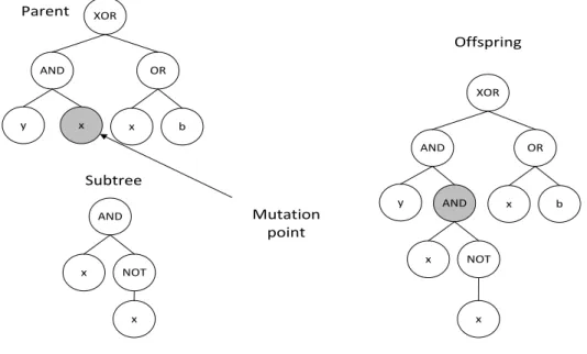
Mutation is a global search operator which creates an offspring by changing components of a single parent selected using one of the selection methods. Different variations of mutation exist such as shrink mutation, point mutation and subtree mutation. Subtree mutation is the most widely used form of mutation. Subtree mutation randomly selects a point within the selected individual (referred to as the mutation point) and replaces the subtree rooted at the mutation point with a newly randomly created subtree [40]. The grow method of population generation is generally used to create the subtree and mutation depth controls the depth of the subtree. Figure 2.4 illustrates the subtree mutation operator. Mutation promotes diversity within the population.

XOR AND x y OR b x AND NOT x x XOR AND y OR b x AND NOT x x Parent Subtree Offspring Mutation point

Figure 2.4: Mutation operation

2.8.3 Crossover

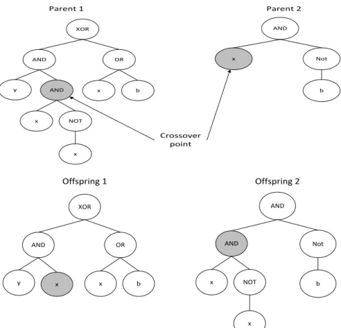
The crossover operator is a local search operator which generates two offspring by exchanging different components (genetic material) between two parents. Two parents are selected using a selection method. A crossover point is randomly selected in each of the two parents. The subtrees at the selected points are exchanged between the two parents to create two offspring [3]. Figure 2.5 Illustrates subtree crossover. Crossover promotes convergence within the population.

15

Figure 2.5: Crossover operation

Crossover has been criticised for being a destructive genetic operator. It has the ability to insert a good building block into an individual that does not make proper use for it. Some authors have argued that the closer a tree is to a solution the more susceptible it is to the destructive effect of crossover [57].

GP Control Models

There are two major models used to control the implementation of GP, the generational model and the steady-state model [3]. In generational GP, individuals in the population are replaced by new individuals after each iteration (termed as a generation). In steady-state GP, the weaker individuals are replaced as the evolutionary process continues. The two models are discussed further below.

16

2.9.1 Generational Model

The generational control model illustrated by Algorithm 2.1 creates a new population from the

previous population [3]. The algorithm randomly initializes the population using one of the initial population generation methods discussed in above. The fitness of the individuals in the generation are evaluated. A selection method is used to select parents which the genetic operators are applied to. The offspring created from the results of genetic operators are inserted in the next population. Iterations of the fitness evaluation and offspring creation are performed until a termination criterion is met.

2.9.2 Steady State Model

Algorithm 2.1 provides the steady-state control GP algorithm. Individuals are selected from the population using selection methods. Genetic operators are performed on the offspring returned from the selection methods [3]. Inverse selection methods are used to select the individual replaced by the offspring.

Generational GP Algorithm

Begin

• Randomly initialize the population

• Repeat

o Evaluate the individual programs in the existing population.

o Select an individual or individuals in the population using selection methods.

o Perform genetic operators on the selected individual or individuals.

o Insert the results of genetic operators into the new population.

• Until a termination criterion is met. End

Return the best individual from the population or solution to the problem.

17

Termination

Termination criteria are measures used to stop the execution of the GP run. Different termination criteria are used within GP. Termination is problem dependent [74]. One of the most commonly used termination criteria is when a solution is found. In the event that a solution is not found, the best individual throughout all the generations is returned. The maximum number of generations can also be used as a termination criterion [40].

Introns and Bloat

Introns are blocks of redundant code that have no effect on the fitness of an individual. (NOT(NOT(X)) is an example of an intron, this block of code does nothing within an individual. Bloat is the exponential program growth without any significant increase in terms of fitness [74]. Rapid increase of introns leads to bloat [3]. Bloat increases exponentially towards the end of a GP run and causes the GP algorithm to be stagnate. Introns can reduce the destructive effects of genetic operators [3]. Different methods such as the use of parsimony pressure have been implemented to reduce bloat. Modularisation has also been used to reduce introns and bloat [49].

Steady-State GP Algorithm

Begin

• Randomly initialize the population

• Repeat

o Randomly choose a subset of existing population to take part in tournament.

o Evaluate subset individuals in the tournament.

o Obtain the winner or winners from subset tournament.

o Perform genetic operations on the winner or winners.

o Apply inverse selection method and replace individual with results of genetic operations.

• Until a termination criterion is met. End

Return the best individual from the population or solution to the problem.

18

Modularisation

Modularisation is commonly used for problem-solving by which functional units of a program are identified and packaged for reuse. The methods encapsulate blocks of code. The encapsulated blocks of code become functions added to the function set and used in the creation of offspring. Modularisation attempts to tackle some of the main problems associated with GP; scaling and inefficiency [3]. Operators such as encapsulation and compression are some of methods which cater for modularisation of programs in GP [2, 40]. Automatically defined functions (ADFs) [8, 39] also caters for modularisation and enables GP to solve problems better [73].

Strengths and Weaknesses of GP

2.13.1 Strengths

• Seeding is used for each GP run and this results in different solutions obtained for each run.

• Easy interpretation and execution of solutions since each solution resembles a computer program.

2.13.2 Weaknesses

• Premature convergence due to lack of genetic diversity and the destructive effect of genetic operators.

• A number of parameters are required to execute a GP run. Optimization of these parameters is essential in order to get the best solution for each problem domain.

• No guarantee that GP will find a global optimum solution due to the stochastic nature of genetic programming.

19

Introduction to Grammatical Evolution

Grammatical Evolution (GE) is a grammar-based variation of Genetic Programming pioneered by Ryan

et al. [59, 76]. GE performs the evolutionary process on variable-length binary strings unlike GP which performs its evolutionary process on actual programs. A bit within the binary string is referred to as an allele and a combination of 8 alleles form a codon. Each binary string codon represents an integer value which is used in a mapping process. GE is inspired by the biological process of generating a protein from the genetic material of an organism follows a similar mapping process. GE unlike GP, is a population of linear genotypic binary strings, which are transformed into functional programs through a genotypic-to-phenotypic mapping process [19, 60]. One of the weakness of GP is the inclusion of redundant code within individuals and GE minimizes redundant code [63].

Overview of the Generational GE Algorithm

The genotypic-to-phenotypic mapping process is governed by the use of a Backus-Naur Form (BNF) grammar, which describes the syntax of the language for the problem. Algorithm 2.3 provides an overview of the generational GE algorithm. The mapping process takes input (BNF grammar) and

produces an output (programs). The created individuals within the population are evaluated for fitness. If a solution is not found within the initial population, the algorithm iteratively selects parents from the population using one of the selection methods. Genetic operators are applied to the

Generational GE Algorithm

Begin

• Randomly initialize the population

• Repeat

o Evaluate the individual programs in the existing population.

o Select an individual(s) in the population using selection methods.

o Perform genetic operations on the selected individuals genotypic string(s).

o Perform mapping process and generate phenotype.

o Insert the offspring into the new population.

• Until a termination criterion is met. End

Return the best individual from the population or solution to the problem.

20

genotypic strings. The mapping process is repeated using the new genotypic strings created after genetic operators. The offspring created are evaluated for fitness. If a solution is not found, the evolutionary process iteratively continues until a termination condition is met.

Representation

Each element of the population is a made up of a randomly generated binary string or denary string. This genotype is then converted to a program by the mapping process. The BNF grammar is used to define the syntax of valid programs [34]. BNF grammar and the mapping process are discussed in detail in the following sections.

2.16.1 BNF Grammar

BNF is a metalanguage (i.e. a language used to describe a language) which consists of the symbol ‘: : =’, denoting “is composed of”; and ‘|’ meaning a choice. It provides a notation for expressing the grammar of a language in the form of production rules. The BNF grammar is made up of the tuple N, T, P, S; where N is the set of all non-terminal symbols, T is the set of terminals, P is the set of productions rules that map N to T, and S is a member of N and the start symbol [60]. An example production rule is of the form:

< expression > : : = < variable > <operator> ge

| ge

Where the non-terminals take the form < expression > (enclosed in angle brackets), and ge is an example of a terminal symbol.

The above production rule states that an < expression > is composed of the non-terminal grammar for <variable> and <operator> as well as the terminal symbol ge. Alternatively, <expression> is composed solely of the terminal symbol ge. Production rules which can generate terminal symbols are referred to as terminal-producing production rules [13].

Terminals in the context of GE are elements that appear in the program produced by GE. These terminals include operators such as *, +, -, / and the values they operate on such as constants, variables. Terminals are not limited to just operators and values; control statements and other structures can be referred to as terminals.

The evolutionary process evolves binary strings and uses the binary strings evolved, the grammar and the mapping process in order to generate complete phenotypic programs [19, 60]. Domain

21

knowledge of a problem can be included within the grammar resulting in the generation of good solutions.

2.16.2 Mapping Process

The mapping process provides a distinction between the search space and the solution space [60]. A suitable BNF must be defined. This grammar specifies the syntax of the phenotypic programs to be produced by the GE. The genotype is used to map the start symbol to the terminals by converting the 8-bit codons into integer values. Taking the leftmost integer codon value, the following mapping function is applied when selecting the appropriate production rule to use:

Rule = Codon Integer Value MOD number of rules for the current non-terminal

Where the MOD function returns the remainder after a division operation (e.g. 3 MOD 2 = 1). The result produced after applying the mapping function corresponds to the production rule used to replace the Start symbol. If the production rule selected contains terminals, the leftmost non-terminal is expanded first. The next integer codon in the chromosome is selected and the mapping function is applied to the next non-terminal. An example of the mapping process is provided below.

If a production rule selected contains non-terminals, the mapping function is iteratively applied to the leftmost nonterminal symbol until one of the following situations arises:

1. When all the non-terminals are converted to elements from the terminal set.

2. The end of the genome is reached and the wrapping operator is applied whereby the mapping is iteratively repeated until a threshold of the maximum number of iterative repeats has been reached during mapping process.

During the mapping process when individuals run out of codons to traverse the genome, the individuals are wrapped around and the codons are reused from the leftmost codon integer value. When the maximum number of wrapping is reached and the individual is still incompletely mapped, the mapping process is stopped and the individual is assigned the lowest fitness value [63]. Another termination criterion of the mapping process is also provided in Genr8 [34] where only the production rules that generate terminals are used to replace the non-terminals in the expression when the threshold of the number of wraps is exceeded.

2.16.2.1 Mapping process example Consider the grammar:

22

Where:

Nonterminal symbols (N) are {exp, op, var}, Terminal set (T) is {+, -, /, *, X, 1},

Start symbol (S) is <exp> and Production rules (P) are:

<exp> : : = <exp> <op> <exp> (0) | <var> (1) <op> : : = + (0) | - (1) | / (2) | * (3) <var> : : = X (0) | 1 (1) Rule Number Choices <exp> 2 <op> 4 <var> 2

Table 2.2: The number of choices for each production rule

Binary String (this is an element of the population)

00010100 00100001 00010010 00010011 00100011 00000111 00001111 00100000 …

Binary to Integer (Denary) conversion Denary Values

23

Start = <exp> 20 % 2 = 0 <exp> <op> <exp> 33 % 2 = 1 <var> <op> <exp> 18 % 2 = 0 X <op> <exp> 19 % 4 = 3 X * <exp> 35 % 2 = 1 X * <var> 7 % 2 = 1

X * 1 Mapping Complete

From the example above the individual created (phenotypic program) from the genotypes and the mapping process is(𝑥𝑥 ∗1). Some of the integer genotypes where not used during the mapping process.

Initial Population Generation and Evaluation

Initial population generation involves creating random chromosomes. The number of chromosomes created is determined by the population size specified in the parameters. Each chromosome is composed of random binary strings. The number of codons specified as a parameter determines the number of binary strings in each chromosome. Each binary string codon in the chromosome is converted to a denary value.

Evaluation of the chromosome takes place by applying the mapping process using the denary values and the grammar provided to generate a program. The wrap-over threshold limit is also specified as one of the parameters before the program executes to ensure the mapping process terminates when a specified number of wraps is exceeded. Evaluation methods, selection methods and termination criterion used within GE are the same as processes described for genetic programming in sections 2.6, 2.7 and 2.10 respectively.

Genetic Operators

Genetic operators are used to create the next generation during the evolution process. Dempsey [19] stated that genetic operators from Holland’s Genetic Algorithm (GA) can be applied to the genotypic strings. Some of the operators employed from GAs are discussed below.

24

2.18.1 Crossover

Crossover generates offspring by combining genotypic material from two parents selected using selection methods. A number of crossover operators have been applied in GE. These include one-point crossover, two-point crossover and homologous crossover.

One-point crossover [60] randomly selects a crossover point in each of the parent binary string codons. Alleles located after the crossover point are swapped between the two individuals to generate two offspring. Figure 2.6 illustrates one-point crossover, where the crossover point is four. The highlighted strings represent alleles from parent 1 and the non-highlighted strings represent alleles from parent 2.

Parent 1 10011010 01010111 …. Parent 2 10111100 00011101 … Offspring 1 10011100 01011101 … Offspring 2 10111010 00010111 ..

Figure 2.6: GE fixed length one-point crossover

For each codon in the parents, two-point crossover randomly selects two crossover points and swaps alleles located between the crossover points [60]. Figure 2.7 illustrates two-point crossover, where the crossover points are at position three and 7.

Parent 1 10011010 01010111 …. Parent 2 10111100 00011101 … Offspring 1 10011100 01011101 … Offspring 2 10111010 00010111 ..

Figure 2.7: GE two-point crossover

Homologous crossover [60] is a modified two-point crossover where the mapping process history of production rules used is kept for each of the individuals. Homologous crossover is applied to the denary values and not the binary strings. The mapping process history of the selected individuals is read from the left until a region of similarity (when the same production rule is selected on both individuals) is found. The first crossover point is selected at the boundary of the region of similarity in

25

both the individuals. The second crossover point is randomly selected from the region of dissimilarity (when the production rules selected are different on both individuals). The codons located between the two crossovers points are then swapped between the individuals. Homologous crossover has two variations, one that swaps blocks of the same size and the other which swaps blocks of differing lengths.

Figure 2.8 illustrates homologous crossover which swaps blocks of the same size.

Figure 2.8: Homologous Crossover

In Figure 2.8, the region of similarity is denoted by the area highlighted in the parent integer codons. The second crossover point is the same in both individuals and the region highlighted in the offspring signifies the codons which were swapped between the two parents.

Homologous crossover requires more memory for execution compared to the other approaches and there is no clear procedure in the event that there is no region of similarity between the parents.

2.18.2 Mutation

A suitable parent is selected using the selection methods and mutation changes a bit or an integer value to another random value within the genotype of the parent generating an offspring. Changes

Crossover Point 1

Crossover Point 2 Parent 1 Integer codons 20 33 18 19 35 07 15 32 …

Production Rules 0 1 0 3 1 1 0 0 …

Parent 2 Integer codons 34 25 15 18 20 06 45 66 … Production Rules 3 2 0 3 2 0 1 1 … Crossover Point 2 Crossover Point 1 Integer codons Offspring 1 20 33 18 19 20 06 45 32 … Offspring 2 34 25 15 18 35 07 15 66 …

26

within the genotypic strings might however have no effect on the phenotype. For example, given the following BNF production rule:

<var> : : = X (0) | 1 (1)

where <var> can either be replaced by variable X or 1. If mutation is performed and each time a binary string which evaluates to an even number is created, the production rule will always select the same variable X. This is termed to as neutral mutation [19].

Different mutation operators are adopted from GA. Some of the mutation operators are discussed below. The bit flip mutation operator inverts the alleles in the binary string meaning that if an allele is a 0, it is changed to 1 or if it is a 1, it is changed to 0. Interchanging mutation randomly selects two points within the binary codon and the alleles corresponding to the positions are interchanged. Flipping mutation randomly generates a binary string (mutation chromosome). The mutation chromosome is aligned with the parent binary codon and traversed from left to right. Whenever a 1 is found in the mutation chromosome, the corresponding bit in the parent binary codon is flipped (0 to1 and 1 to 0) generating the offspring [81]. Figure 2.9 illustrates the different mutation operators discussed above. The highlighted alleles represent where the changes took place.

Bit Flip mutation Parent 10101010 Offspring 01010101

Interchanging mutation

Parent 10111110 Mutation points Points 4 and 8 Offspring 10101111

Flipping mutation

Parent 00101110 Mutation Chromosome 10001001

Offspring 10000001

Figure 2.9: Mutation Operator Variations

Introns and Bloat

Introns are part of the genotypic strings which are not used during the mapping process. If all the non-terminals are not expanded without using all the codons, all the remaining codons are introns. If introns within individuals grow exponentially, they result in bloat as previously discussed in section 2.11. Different methods of controlling introns and bloat have been applied within GE. The use of

27

parsimony pressure and modularisation are among the methods used to control bloat within GE [33, 58].

Strengths and Weakness of GE

GE benefits from some of the strengths and weakness addressed in section 2.13 but it also has other strengths and shortcomings different from GP which are discussed below.

2.20.1 Strengths

• The GE wrapping operator allows short chromosomes to translate into very long expressions and provides an efficient way of avoiding invalid expressions.

• Domain knowledge can be included within the BNF grammar resulting in better tailor-made solutions to problems.

• Bloat does not occur in the phenotype solutions, making solutions produced easy to understand.

2.20.2 Weaknesses

• Longer computational time is required to translate from the genotype to the phenotype during program execution.

• Different genotype strings can map to the same phenotype string reducing the diversity of using different genotypic strings.