Aberystwyth University
Weight selection strategies for ordered weighted average based fuzzy rough
sets
Vluymans, Sarah; MacParthaláin, Neil; Cornelis, Chris; Saeys, Yvan
Published in: Information Sciences DOI: 10.1016/j.ins.2019.05.085 Publication date: 2019
Citation for published version (APA):
Vluymans, S., MacParthaláin, N., Cornelis, C., & Saeys, Y. (2019). Weight selection strategies for ordered weighted average based fuzzy rough sets. Information Sciences, 501, 155-171.
https://doi.org/10.1016/j.ins.2019.05.085
General rights
Copyright and moral rights for the publications made accessible in the Aberystwyth Research Portal (the Institutional Repository) are retained by the authors and/or other copyright owners and it is a condition of accessing publications that users recognise and abide by the legal requirements associated with these rights.
• Users may download and print one copy of any publication from the Aberystwyth Research Portal for the purpose of private study or research.
• You may not further distribute the material or use it for any profit-making activity or commercial gain • You may freely distribute the URL identifying the publication in the Aberystwyth Research Portal
Take down policy
If you believe that this document breaches copyright please contact us providing details, and we will remove access to the work immediately and investigate your claim.
tel: +44 1970 62 2400 email: [email protected]
Weight Selection Strategies for Ordered Weighted
Average Based Fuzzy Rough Sets
Sarah Vluymansa,b,c, Neil Mac Parthal´aind, Chris Cornelisa,∗, Yvan Saeysa,b aDepartment of Applied Mathematics, Computer Science and Statistics,
Ghent University, Belgium
bData Mining and Modelling for Biomedicine, VIB Center for Inflammation Research, Ghent, Belgium
cDepartment of Computer Science and Artificial Intelligence, University of Granada, Spain dDepartment of Computer Science, Aberystwyth University, Wales, UK
Abstract
Fuzzy rough set theory models both vagueness and indiscernibility in data, which makes it a very useful tool for application to various machine learning tasks. In this paper, we focus on one of its robust generalisations, namely or-dered weighted average based fuzzy rough sets. This model uses a weighted approach in the definition of the fuzzy rough operators. Although its efficacy and competitiveness with state-of-the-art machine learning approaches has been well established in several studies, its main drawback is the difficulty in choosing an appropriate weighting scheme. Several options exist and an adequate choice can greatly enhance the suitability of the ordered weighted average based fuzzy rough operators. In this work, we develop a clear strategy for the weighting scheme selection based upon the underlying characteristics of the data. The ad-vantages of the approach are presented in a detailed experimental study. Rather than to propose a classifier, our aim is to present a strategy to select a suitable weighting scheme for ordered weighted average based fuzzy rough sets in gen-eral. Our weighting scheme selection process allows users to take full advantage of the versatility offered by this model and performance improvements over the traditional fuzzy rough set approaches.
∗Corresponding author
Email address: [email protected](Chris Cornelis)
*Manuscript (including abstract) Click here to view linked References
Keywords: fuzzy rough set theory, ordered weighted average, meta-learning
1. Introduction
Uncertainty is a pervasive problem in real-world data. Any machine learning method applied to such data must have a mechanism to handle it effectively. One particular way to do so is to use a mathematical tool that models uncer-tainty. Fuzzy rough set theory [12] offers such advantages. It was proposed as 5
a hybrid form of fuzzy set theory [47] and rough set theory [26] and its central idea is the approximation of fuzzy concepts by means of two fuzzy sets: the fuzzy rough lower and upper approximations. The main limitation of the origi-nal fuzzy rough set model is its high sensitivity to noise. In order to address this shortcoming, several noise-tolerant fuzzy rough set models have been proposed 10
in the literature (e.g. review [18]). Both the traditional model and its later ex-tensions have been used successfully in many different areas of machine learning [37], such as feature selection, instance selection, classification and clustering.
Context. In this paper, we focus on one of these robust extensions: ordered weighted average (OWA) based fuzzy rough sets [10]. It addresses the noise sen-15
sitivity problem of the traditional model by replacing the strict minimum and maximum in its fuzzy rough approximation definitions by appropriate OWA ag-gregations [44], which represent softened versions of these operators. We focus on this model because: (i) it was identified as the most interesting among the al-ternatives compared in [11] and (ii) it has been employed with success for several 20
machine learning tasks, such as imbalanced classification [28, 35, 41], instance selection [33] and missing value imputation [1]. These methods rely on the OWA-based fuzzy rough approximation operators to make class predictions or derive instance or feature quality measures. Although the effectiveness of OWA-based fuzzy rough sets for such techniques has been clearly demonstrated and 25
methods using this model have been shown to outperform the state-of-the-art in these domains, it is not as widely adopted as it could be. We suspect that one of the reasons for this is the requirement to specify the OWA weighting scheme,
the crucial component of this model defining the weights used in its fuzzy rough approximation operators. Several options for these weights are encountered 30
in the literature. However, to date, there are no documented guidelines on which weighting scheme should be chosen within OWA-based fuzzy rough sets. The need for a data-driven weighting scheme selection has been pointed out in e.g. [35] and the optimal choice indeed depends on the data at hand.
Aim. In this work, we remedy exactly this situation and provide a transparent 35
strategy for the weighting scheme selection process. Our research belongs to the domain of meta-learning [24] and we study several existing weight definitions and offer explanations as to why some definitions are preferred over others in specific situations. This paper resolves the missing link in the literature between the theoretical foundations and practical applications of OWA-based fuzzy rough 40
set theory. In this way, we make OWA-based fuzzy rough set theory more accessible to other researchers by removing the often cumbersome weighting scheme selection step. Since it is based on simple dataset properties, there is no true increase in computational cost by following our proposed strategy.
Methodology and contributions. In the experimental evaluation, we compare five 45
different weighting schemes. These include four data-independent versions used in previous studies and a new data-dependent setting proposed in this paper. By including a data-dependent version, we can assess whether considering the underlying data distribution can benefit the OWA-based fuzzy rough model. We will show that this setting is useful overall and also the preferred choice 50
for some challenging datasets, such as those containing only nominal-valued features. Our evaluation demonstrates that no weighting scheme stands out in general, such that no single approach can be selected as a default setting. This reinforces the importance of our proposed selection strategy, that specifies which scheme is preferred in which particular situation. We provide intuitive 55
but thorough explanations for the behaviour of the five schemes. This offers further insight into the mechanisms which underpin OWA-based fuzzy rough sets, a second fundamental contribution of this work. Some conclusions drawn
in this paper are expected to transfer to other applications of OWA operators (including multi-criteria and multi-person decision making [46]) as well, where 60
the weight selection process is always a critical step.
Structure. The remainder of this paper is organized as follows. In Section 2, we recall the definitions of both traditional and OWA-based fuzzy rough sets. Section 3 defines the weighting schemes and offers a comparison between them. In Section 4, we present our proposed strategy for the OWA weight selection 65
process and discuss the benefits and limitations of the different schemes. An important point is the validation of our proposal. This is carried out in Sec-tion 5 and includes the essential evaluaSec-tion on a series of independent datasets and in different machine learning applications. Finally, Section 6 draws some conclusions.
70
2. OWA-based fuzzy rough sets
In this section, we recall the motivation and definition of OWA-based fuzzy rough sets. Section 2.1 describes the traditional fuzzy rough set model and Section 2.2 details the OWA-based generalization. Section 2.3 summarizes how the OWA-based model has been used in various machine learning methods. 75
2.1. Fuzzy rough set theory
Fuzzy rough set theory was proposed in [12] as a hybrid model of fuzzy set theory [47] and rough set theory [26]. Both deal with uncertainty in data, but from different perspectives. Fuzzy set theory models vague or ill-defined con-cepts (e.g. the set of young people) by allowing partial memberships of objects 80
to a set. Such a partial membership degree is a real number between 0 and 1, where the two extremes are interpreted as either complete exclusion from or in-clusion in the set. Rough sets manage data indiscernibility, the situation where the observed features are insufficient to sharply delineate a concept. Rough set theory approximates such an incomplete concept A in two ways. The lower 85
approximation groups all objects certainly belonging toA, while the upper ap-proximation consists of objects possibly belonging toA.
Fuzzy rough set theory introduces fuzziness into rough sets and allows the approximated concept as well as the lower and upper approximations to be modelled as fuzzy rather than crisp sets. To measure the similarity between 90
two objects, a fuzzy relationR(·,·) is used. We consider the implicator/t-norm fuzzy rough set model [27]. An implicatorI: [0,1]2→[0,1] is a fuzzy operator
that is decreasing in its first argument, increasing in the second and satisfies the boundary conditions I(0,0) = I(0,1) = I(1,1) = 1 and I(1,0) = 0. A triangular norm (t-norm)T : [0,1]2 →[0,1] is a commutative and associative
95
fuzzy operator that is increasing in both arguments and satisfies the boundary condition (∀a∈[0,1])(T(a,1) =a). Let A be the (fuzzy) set to approximate. The membership degree ofxto the lower approximation ofAis defined as
A(x) = min
y∈X[I(R(x, y), A(y))], (1) whereXis the full dataset. The membership degree to the upper approximation is given by
100
A(x) = max
y∈X[T(R(x, y), A(y))]. (2) In this paper (and others using fuzzy rough set theory in machine learning), the setAcorresponds to a decision class and is therefore non-fuzzy. The values
A(·) can only be 1 or 0, depending on whether or not an element belongs toA. Taking this into account, expression (1) can be rewritten as
A(x) = min y∈X[I(R(x, y), A(y))] = min min y∈A[I(R(x, y),1)],miny /∈A[I(R(x, y),0)] = min 1,min y /∈A[I(R(x, y),0)] = min y /∈A[ I(R(x, y),0)] = min y /∈A[NI(R(x, y))], (3)
whereNI : [0,1]→[0,1] is the induced negator ofI, defined as (∀a)(NI(a) = 105
is due to the boundary conditionI(1,1) = 1 and the implicator being decreasing in its first argument. In a similar way, expression (2) reduces to
A(x) = max
y∈A[R(x, y)]. (4)
The fuzzy relation used in this paper is defined as follows. Let xand y be two elements in the dataset and F the feature set. The similarity between x
110 andy is computed as R(x, y) = 1 |F | X f∈F Rf(x, y). (5)
The relationRf(·,·) measures the similarity between elements based on feature
f. For a numeric feature, this relation is defined as Rf(x, y) = 1− |xf−yf| range(f),
where xf and yf are the values of xandy for featuref and the denominator
range(f) is its range. Whenf is a nominal feature, we setRf(x, y) to 1 when 115
xf =yf and to 0 otherwise. We have selected relation (5) because it has shown a good behaviour in related studies (e.g. [11, 28, 32]). Some alternatives can be found in e.g. [20]. As we will argue in Section 4.5, we believe that the conclusions drawn in this paper carry over to those settings as well.
2.2. OWA-based model 120
As evident from (3) and (4), the fuzzy rough approximationsA(x) andA(x) depend on the similarity ofxwith a single elementy. This makes the traditional fuzzy rough set model highly susceptible to noise. Several noise-tolerant fuzzy rough set models have been proposed in the literature, including fuzzy variable precision rough sets [48], vaguely quantified fuzzy rough sets [9], β-precision 125
fuzzy rough sets [18] and a data distribution aware model [3]. In this paper, we turn our attention to OWA-based fuzzy rough sets [10], which have been shown to be a preferred alternative among noise-tolerant models [11, 39]. The noise sensitivity of (3) and (4) is addressed by replacing the min and max operators in these definitions by ordered weighted average (OWA,[44]) aggregations. 130
Definition 1. Given a set of values V ={a1, a2, . . . , ap} and a weight vector
W = hw1, w2, . . . , wpi with (∀wi)(wi ∈ [0,1]) and Pp
aggregation ofV using weight vectorW is defined asOWAW(V) =Ppi=1(wibi), wherebi is theith largest value inV.
As Definition 1 indicates, the first step in an OWA process is to sort the 135
values which are to be aggregated. Afterwards, the weights inW are assigned to the values in the ordered sequence and a weighted average is computed. In the OWA-based fuzzy rough set model, the minimum and maximum in (3) and (4) are replaced by appropriate OWA aggregations with weight vectorsWLandWU respectively, such thatorness(WU)≥ 12 ≥orness(WL). The orness measure is a 140
value between 0 and 1 and expresses how similar the weight vector is to the strict maximum. The membership degree to the lower approximation is computed as
A(x) = OWAWL({NI(R(x, y)|y /∈A}). We use the standard negator (NI(x) = 1−x), which is the induced negator of such popular implicators as the Kleene-Dienes, Lukasiewicz and Reichenbach implicators [22]. Consequently, we derive 145
A(x) = OWAWL({1−R(x, y)|y /∈A}). (6) For the upper approximation, we find
A(x) = OWAWU({R(x, y)|y∈A}). (7) By actively including more than one elementy in the calculation ofA(x) and
A(x), the sensitivity to noise and outliers is reduced. This results in the su-perior noise-tolerance of the OWA-based fuzzy rough set model compared to 150
the traditional one. Most commonly, WL consists of increasing weights, such that the largest weight is associated with the minimum, thereby softening the min operator. For the same reason,WU usually contains decreasing weights. A so-calledweighting scheme provides the definitions ofWL andWU. We list and discuss several alternatives in Section 3.
155
2.3. Applications
The survey paper [37] discusses applications of fuzzy rough set theory in various machine learning domains. As noted in the introduction, the OWA-based model has been used in, among others, classification, instance selection
and missing value imputation. These methods internally rely on the OWA-based 160
approximations (6) and (7).
• Classification: in [28] and [41], classifiers for imbalanced data were de-veloped, focusing on two-class imbalanced datasets. They compute the membership degree of a target instance to the OWA-based lower approx-imation of both classes and assign it to the class for which the derived 165
value is largest. The proposed methods deal with the class imbalance problem by using class-dependent weighting schemes. The method of [28] was extended to multi-class imbalanced classification in [38]. Recently, the contribution of [36] proposed a multi-label classifier, applying an OWA-based fuzzy rough neighbourhood consensus.
170
• Instance quality: the proposals of [2], [33] and [35] compute the quality of an instance based on its membership degree to the OWA-based lower and upper approximations of its own class. In [35], the instance quality values are used within a nearest neighbour classifier and assign a more important vote to high quality instances in the class prediction step. The 175
studies of [2] and [33] develop instance selection methods using wrapper approaches.
• Missing value imputation: the authors of [1] proposed missing value imputation methods based on the combination of three fuzzy rough set models, including the OWA-based alternative, with a nearest neighbour 180
classifier. The lower and upper approximations of classes are used inter-nally in the nearest neighbour method, as done in [19].
3. OWA weighting schemes
Expressions (6) and (7) show that the OWA-based fuzzy rough lower and upper approximations depend on weight vectors WL and WU respectively and 185
the weighting scheme that defines them. We list some existing weight defini-tions in Section 3.1 and introduce a new data-dependent version in Section 3.2.
In Section 3.3, we offer a first comparison between the characteristics of the different schemes.
3.1. Data-independent schemes 190
Most weight definitions used in applications of OWA-based fuzzy rough sets only depend onp, the length of the weight vector. We list four of them in this section. For the lower approximation ofAas defined in (6),pequals the size of the complement ofA. For the upper approximation (7),pequals the size ofA. In this section, for a fixed value ofp, the vectorsWL and WU are reversals of 195
each other. Keeping this in mind, we only specify the definition ofWL below.
Strict weights (Strict). As a first option, we include a weight setting that is equal to the traditional model from Section 2.1, for which the lower approximation weight vector isWstrict
L =h0,0, . . . ,0,1i. By only assigning a non-zero weight to the last position, the exact minimum is obtained in (6). It should be clear 200
that the traditional model (3) is indeed a special case of the OWA-based model.
Additive weights (Add). The weight vector for the lower approximation is given by WLadd= 2 p(p+ 1), 4 p(p+ 1), . . . , 2(p−1) p(p+ 1), 2 p+ 1 . (8)
These weights are the normalized version of the vectorh1,2, . . . , p−1, pi. The normalization was carried out to satisfy the conditions in Definition 1. Each 205
weight wi+1 is obtained by adding the constant value p(p2+1) to the previous
weight wi. This means that every next value is assumed to have a constant increase in its relevance to determine the aggregated value.
Exponential weights (Exp). The weight vector for the lower approximation is given by 210 WLexp= 1 2p−1, 2 2p−1, . . . , 2p−2 2p−1, 2p−1 2p−1 . (9)
The weight wi+1 is determined by multiplying wi by the constant factor 2. Every value is deemed twice as relevant for the aggregation as the previous one.
Inverse additive weights (Invadd). The weight vector for the lower approxima-tion is given by WLinvadd= 1 pDp , 1 (p−1)Dp , . . . , 1 2Dp , 1 Dp , (10)
with Dp =Ppi=11i, the pth harmonic number. This vector is the normalized 215 version ofh1 p, 1 p−1, . . . , 1
2,1i. For this setting, as opposed to the other two
dis-cussed above, the relation betweenwi andwi+1 depends oni. To obtainwi+1, wi is multiplied with the factor p−p−i+1i , which increases with i.
3.2. Data-dependent schemes
The four settings detailed in Section 3.1 only depend on the aggregation 220
length and do not take the values to be aggregated into consideration. Although equal-sized sets can contain very different values, the weights used to aggregate them will be the same. In this section, we propose an alternative setting, called Mult, which bases its weights on the values to be aggregated.
LetV =hv1, . . . , vni be the sorted set of values to aggregate. This implies 225
that vn is the smallest value among them. For any other value, its similarity withvn can be computed ass(vi) = 1− |vi−vn|. Since all values inV belong to the unit interval, all valuess(vi) do so as well. Based on these similarity values, we can define a function (forv1 tovn−1)
m(vi) = 1 ifvi=vi+1, s(vi) if vi6=vi+1. (11)
Mult constructs its weights from wn to w1, that is, from the largest to the
230
smallest weight. As a first step, wn is set to 1. Next, wi is calculated by multiplyingwi+1 by the factorm(vi). The vector obtained by this procedure is
Wmult∗ L = *n−1 Y i=1 m(vi), n−1 Y i=2 m(vi), . . . , m(vn−2)·m(vn−1), m(vn−1),1 + . (12)
In order to satisfy the conditions in Definition 1, the final vectorWmult L is the normalized version ofWmult∗
L .
As in Invadd, consecutive weights differ by a factor that depends oni. To determinewi, weightwi+1 is multiplied bym(vi). By using m(vi) rather than s(vi), we ensure that when the valuesviandvi+1are the same, they are assigned
the same weight. If the two values differ,wi+1 is multiplied by the factors(vi).
This factor decreases when i decreases, because values earlier in the ordered 240
sequence V are less similar to the minimum value vn. The decreasing factor means that the weights drop more rapidly toward the beginning of the vector. This is a desirable property, as we expect that the first values inV are far less relevant to the aggregation (a softened minimum) than the later ones.
Mult is the only data-dependent weight setting included in our study. We 245
can find some advances on learning OWA weights from data in the literature, although not in the context of OWA-based fuzzy rough sets. In [25], an OWA weight generation procedure is proposed that maximizes the dispersion of the weights for a given orness value. An analytic solution is offered in [15]. An orness value needs to be specified. Alternatively, the weights can be calculated when 250
a number of samples, in the form ofpvalues and their associated aggregation outcome, are provided. Examples of this approach can be found in [4, 5, 14, 31, 45]. Although interesting, these methods are of no use to us here, because we cannot train the weights with a given orness value or known aggregation outcomes, simply because it is not clear how these parameters should be set. 255
A dependent OWA weight vector was proposed in [43]. This method models a weighted mean of the aggregation values instead of a minimum. The weight of a value is related to its distance to the mean of all values. In [6], a cluster-based OWA aggregation was proposed. To aggregate a set of values, the reliability of each value to the entire set is evaluated based on a clustering of all values. A 260
shortcoming of this procedure is its high computational cost as a result of the clustering step. This was pointed out by [7], which proposed a more efficient procedure to determine the reliability of a value. Like Mult, these methods compute their weights based on the values to be aggregated. Nevertheless, we cannot use them within the OWA-based fuzzy rough approximations, because 265
3.3. Weighting scheme comparison
We study five weighting schemes in this paper: the traditional modelStrict, the data-independent versions Add, Exp and Invadd and our data-dependent proposal Mult. The computational complexity to aggregate p values with an 270
OWA procedure isO(plog(p)) due to the cost of the sorting step. Sorting the values is not required inStrict, such that its cost reduces toO(p).
In Figure 1, we illustrate the weights WL generated by the included alter-natives for some sets with a small number of values to be aggregated. On the horizontal axis, we plot the position of a value in the ordered sequence. The 275
vertical axis represents the weight at a particular position. It is clear that these weight vectors are used to soften the minimum, as they put more emphasis on the higher positions in the ordered sequence, which correspond to lower values (Definition 1). We remind the reader thatStrict always assigns a weight 1 to the last position and weight 0 to all others. This setting is not plotted. 280
In Figures 1a and 1b, we compare the three data-independent settings (Add, ExpandInvadd) for sets with size 5 and 10 respectively. As was clear from their description, the additive weights take on the form of a straight line with slope
2
p(p+1), while the exponential weights are taken from an exponential function
with base 2. The relative weight increase for Exp is the same in each step, 285
that is,wi+1 is obtained by multiplying wi with a constant factor 2. For the inverse additive weights, this relative increase becomes larger when the position
iincreases. It is clear from Figures 1a and 1b that this results in higher weights for the lower positions forInvadd compared to Exp. The exponential weights cancel out the contribution of the values at the lowest positions (in particular 290
whenpis high), whileInvadd always assigns them a non-negligible weight. This is an important difference between these two settings, which will be discussed further in Section 4. Add divides the weights more evenly across the positions than any other setting. This may not always be beneficial. Especially whenpis large, the weight associated with the true minimum may be relatively too low. 295
For large values ofp,Add becomes closely related to a regular average.
1 2 3 4 5 0 0.1 0.2 0.3 0.4 0.5 Position W eigh t
Add Exp Invadd (a)p= 5 1 2 3 4 5 6 7 8 9 10 0 0.1 0.2 0.3 0.4 0.5 Position W eigh t
Add Exp Invadd (b)p= 10 1 2 3 4 5 0 0.1 0.2 0.3 0.4 0.5 Position W eigh t
Mult Exp Invadd (c)V1=h0.9,0.8,0.5,0.2,0.1i 1 2 3 4 5 0 0.1 0.2 0.3 0.4 0.5 Position W eigh t
Mult Exp Invadd (d)V2=h1.0,0.9,0.8,0.7,0.6i
Figure 1: Illustration of the different weight settings.
are related to a nearest neighbour approach. ForStrict, the membership degree ofxto the lower approximation ofAis computed asA(x) = miny /∈A[1−R(x, y)]. This procedure locates the nearest neighbour of xthat does not belong to A. 300
In Exp, the relation with a nearest neighbour technique is more subtle, but is further pronounced as the aggregation lengthp increases. As stated above, whenpincreases,Exp sets several of the lowest weights to zero. For example, when p = 50, only 14 weights in the exponential vector are non-zero. This means that only the 14 nearest elements toxthat do not belong toAare used 305
in the calculation ofA(x). This nearest neighbour characteristic is one of the important aspects which helps to explain the results presented in Section 4.
Figures 1c and 1d compare Mult to Exp and Invadd. These alternatives are related to each other in the sense that a weight can be obtained from the previous or next one by multiplication. The factor in this multiplication is fixed 310
inExp, while it varies forInvaddandMult. We consider two different value sets:
V1 =h0.9,0.8,0.5,0.2,0.1iandV2=h1.0,0.9,0.8,0.7,0.6i. As discussed above,
sinceV1andV2 have the same size, the exponential and inverse additive do not
differ for these two aggregations. TheMult setting on the other hand uses the values inV1 and V2 to determine its weights. The figures show that these are
315
very different forV1 andV2and closely follow the distribution of their values.
4. Weighting scheme selection strategy
In this section, we analyse the performance of the OWA-based lower approx-imation predictor using the five weighting schemes described in Sections 3.1-3.2. Section 4.1 lays out the details of our experimental study and Section 4.2 320
presents an initial high-level comparison of the different OWA weighting schemes. In Section 4.3, we divide the included datasets into eight groups, based on which we can present a selection strategy for the OWA weighting scheme. We explain the observed behaviour of the different weight settings in Section 4.4. Section 4.5 groups some remarks on our chosen approach.
325
4.1. Experimental set-up
We compare the different weighting schemes within OWA-based fuzzy rough sets in a classification setting. We follow [18] and use the lower approximation operator as predictor. To classify an instance x, this classifier computes the membership degreeC(x) of this element for all classes C and assigns xto the 330
class for which this value is highest. It uses expression (6) in this calculation, setting weight vectorWL to one of the five alternatives listed in Sections 3.1-3.2. By doing so, we obtain experimental results of theStrict,Add,Exp,Invadd andMult weighting schemes showing how well they can separate natural groups (classes) of observations. Note that the aim of this paper is not to propose a new 335
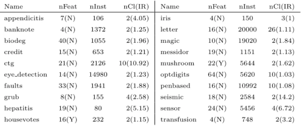
Table 1: Description of the 50 datasets used in the experiments. We list the number of features (nFeat), the number of instances (nInst), the number of classes (nCl) and the IR. Together with the number of features, we specify whether they are all nominal (Y) or not (N).
Name nFeat nInst nCl(IR) Name nFeat nInst nCl(IR) abalone 8(N) 4174 28(689) page-blocks 10(N) 5472 5(175.46) australian 14(N) 690 2(1.25) phoneme 5(N) 5404 2(2.41) automobile 25(N) 159 6(16) pima 8(N) 768 2(1.87) balance 2(N) 625 3(5.88) ring 20(N) 7400 2(1.02) banana 2(N) 5300 2(1.23) saheart 9(N) 462 2(1.89) bands 19(N) 365 2(1.7) satimage 36(N) 6435 6(2.45)
breast 9(Y) 277 2(2.42) segment 19(N) 2310 7(1)
bupa 6(N) 345 2(1.38) sonar 60(N) 208 2(1.14)
car 6(Y) 1728 4(18.62) spambase 57(N) 4597 2(1.54) cleveland 13(N) 297 5(12.62) spectfheart 44(N) 267 2(38.56) contra 9(N) 1473 3(1.89) splice 60(Y) 3190 3(2.16)
crx 15(N) 653 2(1.21) texture 40(N) 5500 11(1)
derma 34(N) 358 6(5.55) thyroid 21(N) 7200 3(40.16) ecoli 7(N) 336 8(28.6) tic-tac-toe 9(Y) 958 2(1.89)
flare 11(Y) 1066 6(7.7) titanic 3(N) 2201 2(2.1)
german 20(N) 1000 2(2.34) twonorm 20(N) 7400 2(1) glass 9(N) 214 6(8.44) vehicle 18(N) 846 4(1.1) haberman 3(N) 306 2(2.78) vowel 13(N) 990 11(1) heart 13(N) 270 2(1.25) wdbc 30(N) 569 2(1.68) ionosphere 33(N) 351 2(1.79) wine 13(N) 178 3(1.48) mammo 5(N) 830 2(1.06) winequal-r 11(N) 1599 6(68.1) marketing 13(N) 6876 9(2.49) winequal-w 11(N) 4898 7(439.6) monk-2 6(N) 432 2(1.12) wisconsin 9(N) 683 2(1.86)
mov lib 90(N) 360 15(1) yeast 8(N) 1484 10(92.6)
nursery 8(Y) 12690 5(2160) zoo 16(Y) 101 7(10.25)
classification method, but rather to develop a strategy to select the weighting scheme for OWA-based fuzzy rough sets within machine learning algorithms in general. Our conclusions transfer to other applications as well (see Section 5.4). We evaluate the performance on 50 datasets (Table 1) by means of 10-fold cross validation. The datasets and partitions were obtained from the KEEL 340
repository atwww.KEEL.es. For each dataset, we list the number of instances, features and classes and specify whether all features are nominal (categorical) or not. Along with the number of classes, we indicate the level of imbalance between them with the imbalance ratio (IR). We compute this measure as the
ratio of the sizes of the largest and smallest classes. For two-class datasets, 345
this coincides with the measure traditionally used in studies on class imbalance [29]. The classification performance of the fuzzy rough lower approximation is evaluated by the balanced accuracy. This metric is defined as the mean of the class-wise accuracies and is not negatively affected by class imbalance. Table 1 shows that several datasets are severely imbalanced. It is accepted within the 350
machine learning community that the traditional global accuracy can provide misleading results on such datasets and should therefore be avoided (e.g. [29]).
4.2. Preliminary performance comparison
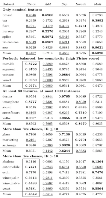
The results for each dataset can be found in Tables 2 and 3. These tables divide the datasets in several groups, which will be described in Section 4.3. 355
The mean balanced accuracy of the fuzzy rough lower approximation predictor is 0.6693 (Strict), 0.6282 (Add), 0.6891 (Exp), 0.6867 (Invadd) and 0.6871 (Mult). The strict model is the best setting for 11 datasets,Add for 8, Exp and Mult for 9 andInvadd for 14. When we derive our weight selection strategy, we do not wish to overfit these results by only focusing on the best setting for each 360
dataset. Instead, we interpret any result that is within 0.05 of the best value as acceptable and any other as poor. We can observe thatStrict performs poorly on 18 datasets,Add on 15,Expon 12 andInvadd andMult on 10.
Based on their average performance, we would conclude that (i)Exp,Invadd and Mult are competitive weight settings and outperform Strict and (ii) Add 365
does not work well. However, we observe thatExp, Invadd andMult perform poorly on at least one fifth of the datasets, meaning that it is not a good idea to select one of these alternatives as a default option. It is also not prudent to excludeAdd from consideration, as it gives the best result on eight datasets. Clearly, the optimal weighting scheme differs between datasets. The study of 370
this phenomenon is our focus. Below, we discuss why certain weighting schemes are preferred in specific situations and present a clear selection strategy.
Table 2: Balanced accuracy results for the datasets in the first five groups of datasets.
Dataset Strict Add Exp Invadd Mult
Only nominal features
breast 0.4946 0.5908 0.5537 0.5826 0.5783 car 0.2459 0.3732 0.2638 0.3474 0.3892 flare 0.1971 0.4179 0.3107 0.4731 0.4274 nursery 0.2267 0.2276 0.2004 0.2268 0.2240 splice 0.5491 0.5972 0.5416 0.5737 0.5770 tic-tac-toe 0.5049 0.5902 0.5211 0.5658 0.5659 zoo 0.9229 0.8526 0.8883 0.8883 0.9621 Mean 0.4487 0.5214 0.4685 0.5225 0.5320 Perfectly balanced, low complexity (high Fisher score)
mov lib 0.8722 0.5889 0.8678 0.8500 0.8589 segment 0.9766 0.8433 0.9745 0.9494 0.9649 texture 0.9869 0.7596 0.9884 0.9664 0.9775 vowel 0.9939 0.6000 0.9859 0.9788 0.9869 Mean 0.9574 0.6980 0.9541 0.9361 0.9470
At least 30 features, at most 1000 instances
derma 0.9554 0.8844 0.9765 0.9689 0.9722 ionosphere 0.8777 0.7321 0.8684 0.8059 0.8311 sonar 0.8515 0.7962 0.8592 0.8928 0.8569 spectfheart 0.6165 0.6387 0.6295 0.7310 0.7100 wdbc 0.9507 0.9313 0.9655 0.9412 0.9473 Mean 0.8503 0.7965 0.8598 0.8679 0.8635
More than five classes, IR≤10
glass 0.7106 0.4659 0.7130 0.6039 0.6236 marketing 0.2101 0.2307 0.2575 0.2701 0.2653 satimage 0.8946 0.6360 0.9026 0.8309 0.8707 Mean 0.6051 0.4442 0.6244 0.5683 0.5865
More than five classes, IR>10
abalone 0.1116 0.0903 0.1150 0.1047 0.1364 automobile 0.7471 0.5243 0.6734 0.6550 0.6600 ecoli 0.7170 0.5598 0.7413 0.7381 0.7476 winequal-r 0.3616 0.2811 0.3590 0.3355 0.3561 winequal-w 0.4498 0.2567 0.4419 0.3863 0.4067 yeast 0.5181 0.3960 0.5359 0.5554 0.5564 Mean 0.4842 0.3514 0.4777 0.4625 0.4772 4.3. Proposed strategy
In Tables 2 and 3, the 50 datasets are divided into eight groups, based on simple and easy-to-compute data characteristics. For each dataset, the highest 375
Table 3: Balanced accuracy results for the datasets in the last three groups of datasets.
Dataset Strict Add Exp Invadd Mult
At most five classes, at most 4000 instances, IR≤2
australian 0.7250 0.8730 0.7946 0.8675 0.8513 bands 0.7308 0.6509 0.7164 0.7173 0.6439 bupa 0.6160 0.6422 0.6498 0.6782 0.6696 contra 0.4030 0.4690 0.4374 0.4836 0.4604 crx 0.7715 0.8695 0.8326 0.8706 0.8650 heart 0.7808 0.8225 0.8058 0.8242 0.8117 mammo 0.7456 0.8205 0.8082 0.8214 0.8114 monk-2 0.7409 0.9052 0.9059 0.9171 0.8144 pima 0.6516 0.7014 0.6754 0.7040 0.6778 saheart 0.5853 0.6620 0.6104 0.6769 0.6315 vehicle 0.6942 0.5670 0.7082 0.6615 0.7006 wine 0.9631 0.9631 0.9673 0.9679 0.9679 wisconsin 0.9617 0.9301 0.9654 0.9497 0.9737 Mean 0.7207 0.7597 0.7598 0.7800 0.7599
At most five classes, at most 4000 instances, IR>2
balance 0.5417 0.7576 0.6378 0.6528 0.7874 cleveland 0.3001 0.2919 0.2855 0.2820 0.2710 german 0.5619 0.6576 0.5750 0.5740 0.5629 haberman 0.5360 0.6363 0.5475 0.5651 0.5267 titanic 0.5211 0.6997 0.6812 0.7109 0.7083 Mean 0.4922 0.6086 0.5454 0.5570 0.5712
At most five classes, more than 4000 instances
banana 0.8728 0.7246 0.8929 0.8848 0.8975 page-blocks 0.7610 0.3198 0.7915 0.5506 0.5978 phoneme 0.8738 0.7730 0.8743 0.8165 0.8455 ring 0.7181 0.5000 0.6924 0.5139 0.5742 spambase 0.8987 0.8027 0.9091 0.8730 0.8447 thyroid 0.6219 0.5280 0.5928 0.5720 0.4340 twonorm 0.9462 0.9757 0.9619 0.9754 0.9723 Mean 0.8132 0.6605 0.8164 0.7409 0.7380
is underlined. Values that are not underlined are considered to correspond to an acceptable alternative to the best setting. For each group of datasets, one particular weighting scheme emerges as the best performing one. These are framed in Tables 2 and 3. We do not only focus on the best performing 380
settings, because we do not wish to overfit this data by proposing strategies that are too specific. We encounter the following groups of datasets, along with their corresponding recommended weighting schemes:
1. Datasets with only nominal features: in our similarity relation (5), the feature-wise similarityRf(x, y) between elementsxandy based on a 385
nominal featuref can only be 0 or 1, depending on whether these elements take on the same value forf. As a result of this lack of variety in similarity values, we can expect that many elements are found at the same distance of a given element. This renders a nearest neighbour approach unsuitable, as reflected by the poor results obtained byStrict andExp.
390
OurMult proposal is able to model the distinct staircase structure in the values to be aggregated and guarantees that equal values are assigned equal weights. Its data-dependent nature makes Mult an appropriate choice for datasets with only nominal features, as evidenced by the re-sults in Table 2. We recommend its use for this group. The rere-sults ofAdd 395
and Invadd are close together and acceptable on average, but they both perform poorly on at least one dataset. For Add, which fails on theflare andzoo datasets, this is explained by the fact that these datasets have a high number of classes (Section 4.4.1). When a small dataset with only nominal features contains only a few classes,Add could be used.
400
2. Perfectly balanced datasets with low complexity: this group con-tains four datasets, for which all classes have the same size. They also have a low data complexity, which can for instance be evaluated by the multi-class Fisher discriminant score [17]. This metric is defined for datasets with only numeric features. A higher value corresponds to a lower com-405
plexity. The four datasets in this group have scores of 2.5413 (mov lib), 15.6143 (segment), 10.2872 (texture) and 2.0389 (vowel), while the average score of the datasets with only numeric features is 1.8451. We recommend the use ofStrict in this case. On these easy datasets, OWA-based fuzzy rough sets do not have a clear advantage over the traditional model. By 410
selectingStrict, the sorting step in the OWA aggregation is avoided. We note that the additive scheme performs very poorly, but this is due to the high number of classes in these datasets (Section 4.4.1). The complexity condition for this group is crucial. For example, datasetmammois almost
balanced, butStrict gives a poor result. Its Fisher score is 0.4926. 415
3. Datasets with at least 30 features and at most 1000 instances: five datasets are included in this group. Themov libdataset from group 2 could be included as well, because it contains 360 instances described by 90 features. We also note that these datasets have only numeric features. Due to their high-dimensional nature, elements are pushed close together 420
(empty space phenomenon). This implies that the values aggregated in the OWA step are more similar to each other than expected in lower dimensional datasets. Add clearly fails in this situation, since it is most related to an average (Section 3.3). For each class, the values in the aggregation will be very similar. If we combine them with a procedure 425
similar to an average, the final values for all classes will be more or less the same. As a result, the prediction byAdd is close to a random guess. The average results of Strict, Exp, Invadd and Mult are close together. We recommend the use of Mult, because it does not perform poorly on any of these datasets. The three other options sometimes give a bad 430
result. Although Mult never obtains the highest balanced accuracy, it is the safest choice. We developedMult in such a way that its weights follow the distribution of the values to be aggregated. We see the benefit of this idea for these complex datasets, where the weights capture important differences and can better discern between classes.
435
4. Datasets with more than five classes and IR ≤10: we recommend the use ofExpfor this group (see Sections 4.4.1 and 4.4.3).
5. Datasets with more than five classes and IR > 10: the tradi-tional model performs best and we recommend the use ofStrict (see Sec-tions 4.4.1 and 4.4.3).
440
6. Datasets with at most five classes, at most 4000 instances and IR
≤2: for these small and balanced datasets, the inverse additive scheme stands out as best performing. We observe that there is only one truly bad weighting scheme for this group, namely Strict. These datasets are relatively easy to handle, because they are not too large, do not have too 445
many classes and are not too imbalanced. This seems to be a setting in which any OWA aggregation performs better than the strict model, as there are no factors that can severely hinder the OWA procedure. The four true OWA aggregations all provide relatively good results. Their average balanced accuracies are not very different. Nevertheless, Add, 450
Exp and Mult fail on some of these datasets, while Invadd never does. Consequently, we advise the use of the latter for this group. We note that Invadd has also come out as best general performing setting in previous studies (e.g. [32, 40]) and its strength is most evident for this group of datasets. From the 14 datasets in which Invadd attained the highest 455
balanced accuracy, nine are contained in this group. When there are no prior challenging factors (e.g. large size, many classes, class imbalance), Invadd seems to be a good default choice.
7. Datasets with at most five classes, at most 4000 instances and IR>2: Add shows the best performance on this group of datasets. Their 460
strength in the presence of class imbalance is explained in Section 4.4.3. 8. Datasets with at most five classes and more than 4000 instances:
when a dataset contains many instances, using exponential weights is a good option. We explain this behaviour in Section 4.4.2.
We realise that the thresholds selected to create these groups may seem artificial, 465
but they are based on the results in Tables 2 and 3 and will be justified in Section 4.4 and validated in Section 5. The user can also relax these guidelines, for instance by replacing ‘more than five classes’ by ‘many classes’, ‘at most 4000 instances’ by ‘a small dataset’ and so on. Our main priority is to capture the general behaviour of the weight settings. In order to apply our proposed 470
strategy in practice in a machine learning method using OWA-based fuzzy rough sets, a weighting scheme selection step should be implemented before the main algorithm. Based on the included easy-to-compute dataset characteristics, the method would first evaluate whether the dataset at hand belongs to the first group. If not, it verifies its membership to the second group and the third one 475
after that. When the dataset does not belong to any of the first three groups, the method decides to which of the final five it belongs, which are mutually exclusive. Having done so, the weight vector in (6) is set according to the weighting scheme advised for the selected group and the main algorithm devised by the user can be run. Examples of this approach are provided in Section 5.4.
480
4.4. Explaining the observed behaviour
In this section, we answer some questions related to the observations made above and that naturally arise when studying the results in detail. These pro-vide further insight in the performance of the different weighting schemes. We consider the following three challenges: a high number of classes (Section 4.4.1), 485
a high number of instances (Section 4.4.2) and class imbalance (Section 4.4.3). Our analysis contains several important take-away messages for researchers who wish to use OWA-based fuzzy rough sets.
4.4.1. High number of classes
In this paper, we interpret a high number of classes as ‘more than five’. This 490
concerns all datasets in groups 4 and 5 by definition. Apart from these, the four datasets in group 2 all contain more than five classes as well. In group 1, datasets flare and zoo have six and seven classes respectively and the derma datasets from group 3 also contains six. In all, of the 50 datasets in Table 1, a subset of 16 have more than five classes. The average balanced accuracy of 495
the weight settings over these datasets are 0.6641 (Strict), 0.5242 (Add), 0.6707 (Exp), 0.6597 (Invadd) and 0.6733 (Mult). Strict obtains the best result for six datasets,Mult andExp each obtain the best result on four, whileInvadd takes first place on the remaining two. Add has a poor result on 14 out of the 16 datasets. The other four alternatives each fail on two datasets. The following 500
questions need to be addressed:
1. Why doesAdd not perform well when the number of classes is high? 2. In datasets with many classes, why areStrict andExp the preferred
We provide an answer to these two questions in the separate paragraphs below. 505
Question 1. Based on its mean balanced accuracy and the number of datasets on which it performs poorly,Add is highly inferior to the other weight settings (includingStrict) when the number of classes is high. The reason for its bad performance is that there is too little difference in the sets of values to aggregate, that is, these sets have a high degree of overlap. Assume that there are six classes 510
in the dataset (C1toC6). In (6), the membership degree ofxtoCiis computed by aggregating the values 1−R(x, y) for instances y in any of the five other classes. This implies an overlap of four classes between the aggregation sets of
Ci and Cj. For example, C1(x) and C2(x) both use all values 1−R(x, y) in
classes C3, C4, C5 and C6. The only difference between the value vectors of
515
C1(x) andC2(x) is that the former uses classC2 and the latter classC1.
The increased expected overlap between the value vectors in the lower ap-proximation aggregations holds for the OWA model in general and is not specific forAdd. Nevertheless, sinceAdd assigns a large relative importance to all values (Section 3.3), the high overlap implies that the aggregated values for the differ-520
ent classes will be close together. Consequently, the ability to discern between classes decreases and prediction errors are made. Other weight settings are hin-dered less by the overlap, because their weight distribution is highly different to that ofAddand places a clearer emphasis on the minimum (Section 3.3). On top of the overlap problem, a high number of classes also implies an increase in the 525
size of the sets to aggregate. When the additive weight vector becomes longer, its behaviour approaches that of a regular average, which further accentuates the issue that the valuesCi(x) are not sufficiently distinct.
Question 2. In our strategy presented in Section 4.3, we recommendStrict or Exp for datasets with more than five classes (groups 4 and 5). Table 2 shows 530
that these are indeed the preferred configurations for such datasets in this study. Although they have been computed over a larger set of datasets, the average results listed at the beginning of this section confirm this.
Aside from the poor performance ofAdd, Table 2 also indicates thatInvadd and Mult perform relatively less strongly on the datasets in groups 4 and 5. 535
As explained in our answer to the previous question, when there are many classes in the dataset, there is a large overlap between the value vectors in the lower approximation computations. Although not to such an extent asAdd, the Invadd andMult settings also assign non-negligible weights to all values to be aggregated. As a result, they are also at risk for aggregated class approximation 540
values that are too close to each other to adequately distinguish between them. MultoutperformsInvadd, because its weights are set up to decrease more rapidly going from right to left in the weight vector.
Strict andExp are nearest neighbour approaches and only consider a small portion of the values in their aggregation step. This helps them to avoid the 545
overlap problem and explains why they are the preferred weight setting in this situation. We make a further distinction between groups 4 and 5 based on the degree of imbalance in the dataset. The reason whyStrict is preferred overExp when the IR of a dataset is large is discussed in Section 4.4.3.
4.4.2. High number of instances 550
In this study, we put the threshold of a high number of instances to 4000. We realize that this is a small number in the big data era, but it is sufficiently large considering the characteristics described in Table 1. There are 13 datasets in our study with a size larger than 4000. These include the seven datasets from group 8, marketing and satimage from group 4, abalone and winequal-w 555
from group 5, nursery from group 1 and texture from group 2. The average balanced accuracy of the weight settings on these datasets is 0.6594 (Strict), 0.5250 (Add), 0.6631 (Exp), 0.6132 (Invadd) and 0.6190 (Mult). Strict andExp are clearly preferable in this case and the latter is the overall best choice.
The difference between Strict and Exp on the one hand and Add, Invadd 560
andMult on the other is that the nearest neighbour nature of the former two can cancel out the contribution of some instances (Section 3.3). ForStrict, this is always the case, as it has zero weights for all but one position. ForExp, zero
weights occur when the length of the vector increases, when due to its rapid (exponential) descent in weights from right to left in the vector WL, only a 565
small portion of values are assigned non-zero weights.
A larger dataset size implies a larger length of the weight vectors. The experimental results show that a nearest neighbour approach is more suitable for this situation than a full OWA aggregation, which takes all values into account. Add,Invadd andMult lose some of their characteristics, because they insist on 570
assigning some weight to all values. As the aggregation length becomes larger, important values (i.e. those close to the minimum) are assigned increasingly smaller weights to accommodate for this property, since OWA weights always sum to one (Definition 1). This is most prominently noticeable in Add, where the weight vector almost flattens out to a regular average.
575
The reason why Exp is preferred over Strict is the same as why k-nearest neighbour classification (kNN, with k > 1) is preferred over 1-nearest neigh-bour classification. It is more robust against noise and makes more confident predictions by relying on multiple near elements. Furthermore, weighted kNN is often favoured over uniformkNN, because the former assigns relatively more 580
importance to nearer neighbours in its predictions [13].
4.4.3. Class imbalance
We have used the IR of a dataset on two occasions in our weight selection strategy: to make a distinction between groups 4 and 5 on the one hand and between groups 6 and 7 on the other. In this section, we explain why the weight 585
choice can depend on the IR of a dataset. We answer two questions:
1. In datasets with a low number of classes and instances, why isAdd the only good choice when the dataset is at least mildly imbalanced?
2. In datasets with many classes, why is Strict preferred in case of large imbalance andExp in case of small to mild imbalance?
590
Question 1. This question pertains to datasets with at most five classes, at most 4000 instances and an IR of at least two. The latter implies that the largest class is at least twice as large as the smallest class. In Table 3, five datasets have been assigned to group 7. Aside from these,breast,car andsplice from group 1 595
andspectfheart from group 3 also have the properties listed above. The average balanced accuracy of the weight settings on these 9 datasets is 0.4852 (Strict), 0.5826 (Add), 0.5240 (Exp), 0.5577 (Invadd) and 0.5679 (Mult). The additive scheme attains the best average result and the highest number of wins (4 out of 9). AlthoughAdd appeared to be an inferior weight alternative in Section 4.2, 600
it is clearly dominant on small, imbalanced datasets. We expect that the bad performance ofStrict andExp is due to their relation to the nearest neighbour classifier and the sensitivity of the latter to class imbalance.
Considering the results in more detail, we noticed that the other OWA alter-natives often fall in the trap of class imbalance, that is, they assign instances to 605
a majority class too easily. This implies a high accuracy for the majority class, but severely lower accuracies for minority classes. Our use of the balanced ac-curacy guarantees that a bad performance on small classes is not overshadowed by a good one on large classes. Add usually has similar accuracy rates for all classes in these datasets, reflected in its superior balanced accuracy values. 610
Expression (6) shows that the membership degree to the lower approximation of a classC is calculated by aggregating values based on elements that do not belong toC. Assume that the dataset contains two classesC1andC2and that
the former is the majority class. Because of the above condition on the IR, this means thatC1 is at least twice as large as C2. To classify an instance x,
615
the predictor computes two values: C1(x) = OWAWL({1−R(x, y)|y ∈ C2}) and C2(x) = OWAWL({1−R(x, y)|y ∈ C1}). Due to the difference in class sizes, the first aggregation is taken over far less values than the second. The largest influence of this fact is felt byAdd. As discussed above, the longer the additive weight vector becomes, the closer it is to a regular average. Since the 620
aggregation lengths can be very different, the characteristics ofAdd on either class can severely vary as well. The longer aggregation (C2(x)) will be far closer
to an average of its values than the shorter one (C1(x)). This difference in the
treatment of classes is far less pronounced for the other OWA alternatives and in Strict it is even non-existent. Here lies the key to why Add is preferred in 625
the presence of class imbalance: its high sensitivity to the length of the vector makes it process minority and majority classes very differently. It does not allow for majority elements to dominate the minority elements. The contributions of majority instances are almost averaged in the calculations, while those of minority elements are aggregated with a truer OWA aggregation. A similar 630
conclusion holds when there are more than two classes.
In summary, like many other classifiers, the lower approximation predictor is sensitive to class imbalance. The additive weighting scheme inherently treats majority and minority classes differently, which is why it is the preferred choice here. We note that the work of [28] provides a more detailed study on appro-635
priate OWA weight vectors when dealing with two-class imbalanced datasets.
Question 2. This question relates to datasets with more than five classes. We recommend to useExpwhen the IR is at most 10 (group 4) andStrict otherwise (group 5). In Section 4.4.1, we have already explained whyStrict andExp are the best weight options for datasets with more than five classes. For datasets 640
with a moderate IR,Exp is preferred over Strict for the same reason as given in Section 4.4.2, namely the higher prediction confidence and robustness when more than one near neighbour is used in the classification process. For a highly imbalanced dataset, the strict model is a better option. This is due to the class imbalance problem, which has a larger influence onkNN (with k >1) than on 645
1NN.Exploses some of its strength when the imbalance becomes large.
4.5. Remarks on our approach
As explained in Section 4.1, we have used the prediction performance of the OWA-based lower approximation to study the differences between the five weighting schemes. Machine learning methods using OWA-based fuzzy rough 650
relevant for practical applications. We have clearly explained the effects of the weights in different situations. However, it is important to reflect on two aspects affecting the classifier performance: our selection of the five weighting schemes and similarity measure (5).
655
Evaluated weighting schemes. Additional weighting schemes can be found in the literature or devised by the reader. However, in light of the different prop-erties exhibited by each scheme (Sections 3.1-3.3), we feel that we have made an appropriate selection. When the reader wishes to assess the adequacy of their custom weighting scheme within OWA-based fuzzy rough sets, they should be 660
able to do so based on our discussion in Sections 4.3-4.4. We have based our-selves on the general defining characteristics of the schemes, in particular in Section 4.4, and our conclusions should carry over to other alternatives as well. Instance similarity. We have chosen to fix the fuzzy relation measuring instance similarity to expression (5). This is a reasonable and intuitive similarity mea-665
sure, which has been used in previous studies on fuzzy rough classifiers as well. Alternatives exist, but we do not expect that our observations and conclusions in Sections 4.3-4.4 will greatly change when a different (sensible) relation is used. When an alternative similarity measure is more suitable for a particular dataset, the performance of the classifier will improve, but we believe that the relative 670
rankings of the weighting schemes will remain the same. Since we focus on the latter aspect, optimizing the similarity relation is of secondary importance and our default use of (5) is justified. Our conclusions in the previous sections are not strongly based on the instance similarity values. Naturally, like the nearest neighbour classifier, any fuzzy rough classifier may benefit from the application 675
of metric learning [23]. A user that wishes to apply our simple classifier in a pre-diction task can opt to use our guidelines in conjunction with a data-dependent similarity measure derived with a metric learning technique.
5. Validation of the proposed strategy
We proceed with the validation of our proposal and do so in several steps: 680
1. Section 5.1: we first evaluate its performance on the 50 datasets in Table 1.
2. Section 5.2: next, we compare our manually detected trends with those extracted by a decision tree meta-learner.
3. Section 5.3: the third, important step is to validate the weight selection 685
strategy on independent datasets that were not used in Section 4. 4. Section 5.4: finally, we consider two other applications aside from
clas-sification and show that our guidelines are useful in these settings as well. We can analyse the difference in performance of our selection strategy and the fixed weight definitions by means of the Wilcoxon test [42]. This non-690
parametric test compares the results of methods M1 and M2 on n datasets. For each dataset, the difference in performance is computed by subtracting the result of M2 from that of M1. Afterwards, these differences are ranked from small to large in absolute value. The smallest difference is assigned rank 1, the largest rankn. R+and R−are computed as the sum of the ranks of the positive 695
and negative differences respectively. A higher value of R+ is interpreted as a
better performance of M1 compared to M2. A test statistic and p-value can be computed based on R+ and R−. When R+ >R− and the p-value is smaller than the significance levelα, it can be concluded that M1 performed significantly better than M2 on this group of datasets. In this paper, we useα= 0.05. 700
5.1. Data from Table 1
If we follow our proposed strategy to select a weight setting for the 50 datasets in Table 1, the mean balanced accuracy increases to 0.7109. This is a noticeable increase compared to the highest value of 0.6891 in Section 4.2. On 25 out of the 50 datasets, our weight selection strategy chooses the weight 705
setting with the best performance. On the 25 remaining ones, an alternative for which the balanced accuracy is at most 0.05 lower is chosen.
To verify whether the increase in balanced accuracy is statistically signifi-cant, we use our proposal as M1 in the Wilcoxon test and compare its perfor-mance to that of the five weight settings. The test shows that the proposed 710
strategy outperforms every weight setting with statistical significance. In par-ticular, using each of the five alternatives as M2, we find p-values of 0.000071 for Strict (R+ = 1048.5, R− = 226.5), 0.00000041 for Add (R+ = 1127.0,
R− = 98.0), 0.000466 for Exp (R+ = 999.5, R− = 275.5), 0.002114 forInvadd (R+ = 921.0, R− = 304.0) and 0.002074 for Mult (R+ = 956.0, R− = 319.0). 715
This good behaviour is not unexpected, as our strategy was derived based on the performance of the weight settings on these datasets. In Section 5.3, we validate our proposed strategy on independent datasets.
5.2. Decision tree
Our selection strategy in Section 4.3 has been constructed manually. We 720
decided that any result that is within 0.05 of the best value for a dataset is acceptable. By doing so, we avoided overfitting our data and were able to construct sufficiently general and understandable weight selection rules. We did not aim to obtain the best overall result, but rather to avoid poor results.
Another option is to construct a meta-dataset, based on which the weight 725
rules can be learned automatically. This dataset contains 50 entries, each corre-sponding to one dataset. We can use the data characteristics used in Section 4.3 (e.g. number of classes) as features. The class label of an entry is the name of the best performing weight setting for that dataset. To extract rules, a decision tree can be trained on the meta-dataset. The resulting tree model can be used 730
to assign a weight setting to a new dataset based on its characteristics. Although it removes the subjective aspect of our manual derivation, a limi-tation of this automated procedure is that there is no possibility to incorporate the same flexibility as before and accept slightly sub-optimal results. Using the meta-dataset corresponds to a different goal, namely to select the best weight 735
setting as often as possible. The downside is that there is no safety net: if the best setting is not selected, a very poor alternative may very well be chosen.
We have used the rpart function from the rpart package in R [30] to train a decision tree on the meta-dataset. All parameters were set to their default settings, apart from ‘minbucket’, which we set to four. For this value, the 740
Figure 2: Decision tree learned from the meta-dataset. For each internal node, the left child fulfils the condition, the right child does not.
tree has eight leaf nodes. We deemed this appropriate, because we used eight groups of datasets as well. As splitting features, the tree can select the number of instances, the number of classes, the IR and whether or not there are only nominal features in a dataset. Figure 2 presents the resulting decision tree.
The tree detects the same general trends as we did. Its first split is made on 745
the number of classes. We interpreted up to five classes as a small number, but the tree considers any number larger than two as high. An explanation may be that many of our datasets consist of only two classes (24 out of 50).
In datasets with a small number of classes and many instances,Exp should be used. We modelled this as well and explained this behaviour in Section 4.4.2. 750
When both the number of classes and instances are small,Invadd is used when the classes are more or less balanced andAdd when they are not. This roughly corresponds to groups 6 and 7 in Section 4.3. We used the threshold 2 to decide when the imbalance is too large, the tree uses 2.22.
For datasets with only nominal features, the tree selects the additive scheme. 755
Table 2 shows thatAdd indeed has the most wins on these datasets, but gives a bad result on some of them as well. We compromised and selectedMult. The
decision tree cannot do so, because it focuses on the best performing settings. In datasets with a higher number of classes, we made a division based on the IR. This does not happen in the decision tree. It groups all datasets with 760
more than two classes in the right sub-tree, while we only considered the subset of datasets with more than five classes. The tree again advises the use of Exp when the dataset is large (see Section 4.4.2). Among the remaining datasets, a distinction is only made based on the number of classes. Mult is used for datasets with three, four or at least seven classes andStrict when there are five 765
or six. This division seems somewhat artificial and cannot be easily explained. The tree is probably overfitting the meta-dataset.
The mean balanced accuracy on the datasets in Table 1 using the weight settings provided by the tree is 0.7089 and the best scheme is selected for 27 datasets. In Section 5.1, our weight scheme selection strategy selected the best 770
setting on 25 datasets and attained a mean balanced accuracy of 0.7109. Al-though it leads to fewer wins, its power to compromise allows our proposal to perform better on average. Furthermore, it never selects a poor performing scheme on the 50 datasets, while the tree does so on four of them. Aside from their performance, our strategy can be favoured over the decision tree for a 775
second reason: it is easier to understand and explain.
5.3. Independent data
In this section, we evaluate the performance of our proposed strategy on independent datasets, that is, datasets that have not been used in this study thus far. This evaluation will further reinforce the demonstrated efficacy and 780
validity of our proposal. The 20 datasets used in this section are listed in Table 4 and are representatives of the eight groups defined in Section 4.3. They were obtained from the KEEL, UCI and Weka platforms. These datasets and their partitions can be downloaded fromhttp://www.cwi.ugent.be/sarah.php.
We present the balanced accuracy values of this evaluation in Table 5. Apart 785
from the results obtained using our proposed strategy, the table also shows the performance of the five individual weight settings. As before, the best value
Table 4: Description of the 20 independent datasets used in Section 5.3 We list the number of features (nFeat), the number of instances (nInst), the number of classes (nCl) and the IR. Together with the number of features, we specify whether they are all nominal (Y) or not (N).
Name nFeat nInst nCl(IR) Name nFeat nInst nCl(IR)
appendicitis 7(N) 106 2(4.05) iris 4(N) 150 3(1)
banknote 4(N) 1372 2(1.25) letter 16(N) 20000 26(1.11) biodeg 40(N) 1055 2(1.96) magic 10(N) 19020 2(1.84) credit 15(N) 653 2(1.21) messidor 19(N) 1151 2(1.13) ctg 21(N) 2126 10(10.92) mushroom 22(Y) 5644 2(1.62) eye detection 14(N) 14980 2(1.23) optdigits 64(N) 5620 10(1.03) faults 33(N) 1941 2(1.88) penbased 16(N) 10992 10(1.08)
grub 8(N) 155 4(2.58) seismic 18(N) 2584 2(14.2)
hepatitis 19(N) 80 2(5.15) sensor 24(N) 5456 4(6.72) housevotes 16(Y) 232 2(1.15) transfusion 4(N) 748 2(3.2)
for each dataset is shown in bold typeface, while any value that is more than 0.05 lower than this optimum is underlined. The advantages of our proposal are clear. We obtain the highest balanced accuracy on average, the most wins 790
and the fewest poor results. The table also shows that our selection strategy is not infallible either, as it does not perform well on themushroom dataset. The Mult setting is selected, because this dataset contains only nominal features. However, if we were to ignore this particular guideline, mushroom would be assigned to group 8, because it has 2 classes and 5644 instances. In this case, it 795
would be processed withExp, which is the preferred setting for this dataset. We compare the performance of our proposal to the five weight settings using a Wilcoxon test. We can conclude that it performs significantly better than Strict (R+ = 167.5, R− = 42.5, p= 0.01821), Add (R+ = 178.0, R− = 12.0,
p = 0.00027) and Mult (R+ = 165.5, R− = 44.5, p = 0.02272). We cannot 800
conclude that our approach provides a significantly better result thanInvadd (R+ = 144.5, R− = 65.5, p = 0.14827) or Exp (R+ = 122.5, R− = 87.5,
p= 0.47034), although the higher values for R+ do indicate a preference in our
favour. Table 5 also demonstrates that a higher balanced accuracy is obtained on average in this case, as well as a higher number of wins and lower number 805
Table 5: Balanced accuracy results of the classification by the OWA-based fuzzy rough lower approximation operator on independent datasets. With the results of our weight selection strategy, we list the selected weight setting between brackets.
Dataset Strict Add Exp Invadd Mult Proposal
appendicitis 0.7514 0.7938 0.7479 0.7868 0.7542 0.7938(A) banknote 0.9987 0.9247 0.9987 0.9961 0.9987 0.9961 (I) biodeg 0.8153 0.7139 0.8381 0.8216 0.8513 0.8216 (I) credit 0.8194 0.8695 0.8582 0.8704 0.8571 0.8704(I) ctg 0.7379 0.3999 0.7301 0.6283 0.6793 0.7379(S) eye detection 0.8456 0.5903 0.8615 0.8147 0.7226 0.8615(E) faults 0.9897 0.6748 0.9919 0.9611 0.9904 0.9611 (I) grub 0.2638 0.3963 0.3075 0.3638 0.3500 0.3963(A) hepatitis 0.8184 0.8232 0.8199 0.8633 0.7715 0.8232 (A) housevotes 0.9137 0.9017 0.9209 0.9125 0.9125 0.9125 (M) iris 0.9333 0.9533 0.9400 0.9533 0.9533 0.9333 (S) letter 0.9428 0.6124 0.9632 0.9556 0.9537 0.9632(E) magic 0.8129 0.7606 0.8384 0.8126 0.7907 0.8384(E) messidor 0.6282 0.6056 0.6534 0.6546 0.6638 0.6546 (I) mushroom 0.9593 0.8026 0.9749 0.9713 0.9034 0.9034 (M) optdigits 0.9843 0.9094 0.9857 0.9798 0.9834 0.9857(E) penbased 0.9936 0.7624 0.9939 0.9671 0.9902 0.9939(E) seismic 0.5514 0.7015 0.5299 0.5872 0.4998 0.7015(A) sensor 0.9224 0.7393 0.9255 0.9024 0.9080 0.9255(E) transfusion 0.5708 0.6528 0.6048 0.6745 0.6047 0.6528 (A) Mean 0.8126 0.7294 0.8242 0.8238 0.8069 0.8363 # best/poor 2/4 4/12 10/3 4/2 4/6 11/1
is based on simple data characteristics, the computation time to assess which weighting scheme should be selected based on our instructions is negligible.
The aim of this paper has been to provide a better understanding of the impact of the different weighting schemes on the OWA-based fuzzy rough set 810
model and advise how to make an appropriate choice between them. Our ob-jective has not been to develop a new state-of-the-art classifier. Nevertheless, we briefly remark that the use of our guidelines lifts the classification result of the simple fuzzy rough lower approximation classifier to the level of the random forest method [8]. This is a far more complex model and is generally accepted as 815
a strong classifier. Using the default random forest method from the Weka plat-form [16] with ten decision trees, the mean balanced accuracy on the datasets