DOI 10.1007/s10994-011-5272-5
Statistical topic models for multi-label document
classification
Timothy N. Rubin·America Chambers· Padhraic Smyth·Mark Steyvers
Received: 1 October 2010 / Accepted: 9 November 2011 / Published online: 29 December 2011 © The Author(s) 2011
Abstract Machine learning approaches to multi-label document classification have to date
largely relied on discriminative modeling techniques such as support vector machines. A drawback of these approaches is that performance rapidly drops off as the total num-ber of labels and the numnum-ber of labels per document increase. This problem is amplified when the label frequencies exhibit the type of highly skewed distributions that are often observed in real-world datasets. In this paper we investigate a class of generative statistical topic models for multi-label documents that associate individual word tokens with different labels. We investigate the advantages of this approach relative to discriminative models, par-ticularly with respect to classification problems involving large numbers of relatively rare labels. We compare the performance of generative and discriminative approaches on docu-ment labeling tasks ranging from datasets with several thousand labels to datasets with tens of labels. The experimental results indicate that probabilistic generative models can achieve competitive multi-label classification performance compared to discriminative methods, and have advantages for datasets with many labels and skewed label frequencies.
Keywords Topic models·LDA·Multi-label classification·Document modeling·Text classification·Graphical models·Probabilistic generative models·Dependency-LDA
Editors: Grigorios Tsoumakas, Min-Ling Zhang, and Zhi-Hua Zhou. T.N. Rubin (
)·M. SteyversDepartment of Cognitive Sciences, University of California, Irvine, Irvine, CA 92697, USA e-mail:[email protected]
M. Steyvers
e-mail:[email protected] A. Chambers·P. Smyth
Department of Computer Science, University of California, Irvine, Irvine, CA 92697, USA A. Chambers
e-mail:[email protected] P. Smyth
1 Introduction
The past decade has seen a wide variety of papers published on multi-label document classi-fication, in which each document can be assigned to one or more classes. In this introductory section we begin by discussing the limitations of existing multi-label document classification methods when applied to datasets with statistical properties common to real-world datasets, such as the presence of large numbers of labels with power-law-like frequency statistics. We then motivate the use of generative probabilistic models in this context. In particular, we illustrate how these models can be advantageous in the context of large-scale multi-label corpora, through (1) explicitly assigning individual words to specific labels within each document—rather than assuming that all of the words within a document are relevant to each of its labels, and (2) jointly modeling all labels within a corpus simultaneously, which lends itself well to the task of accounting for the dependencies between these labels.
1.1 Background and motivation
Much of the prior work on multi-label document classification uses data sets in which there are relatively few labels, and many training instances for each label. In many cases, the datasets are constructed such that they contain few, if any, infrequent labels. For example, in the commonly used RCV1-v2 corpus (Lewis et al.2004), the dataset was carefully con-structed to have approximately 100 labels, with most labels occurring in a relatively large number of documents.
In other cases researchers have typically restricted the problem by only considering a subset of the full dataset. As an example, a popular source of experimental data has been the Yahoo! directory structure, which utilizes a multi-labeling classification system. The true Yahoo! directory structure contains thousands of labels and is a very difficult classification problem that traditional classification methods fail to adequately handle (Liu et al.2005). However, the majority of multi-label research conducted using the Yahoo! directory data has been performed on the set of 11 sub-directory datasets constructed by Ueda and Saito (2002). Each of these datasets consists of only the second-level categories from a single top-level Yahoo! directory, leaving only about 20–30 labels in each of the classification tasks. Furthermore, many of the publications (e.g., Ueda and Saito2002; Ji et al.2008) that use the Yahoo! subdirectory datasets have removed the infrequent labels from the evaluation data, leaving between 14 and 23 unique labels per dataset. Similarly, experiments with the OHSUMED MeSH terms (Hersh et al.1994) are typically performed on a small subdirectory that contains only 119 out of over 22,000 possible labels (for a discussion, see Rak et al. 2005).
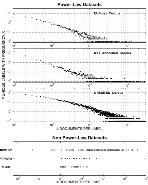
In contrast to the datasets typically utilized in research, multilabel corpora in the real world can contain thousands or tens of thousands of labels, and the label frequencies in these datasets tend to have highly skewed frequency-distributions with power-law statistics (Yang et al.2003; Liu et al.2005; Dekel and Shamir2010). Figure1illustrates this point for three large real-world corpora—each containing thousands of unique labels—by plotting the number of labels within each corpus as a function of label-frequency. For each corpus, the total number of labels is plotted as a function of label-frequency on a log-log scale (i.e., more precisely, number of unique labels [y-axis] that have been assigned tokdocuments in the corpus is plotted as a function ofk[x-axis]). Of note is the power-law like distribution of label frequencies for each corpus, in which the vast majority of labels are associated with very few documents, and there are relatively few labels that are assigned to a large number of documents. For example, roughly one thousand labels are only assigned to a
Fig. 1 Top: The number of unique labels (y-axis) that haveKtraining documents (x-axis) for three large-s-cale multi-label datasets. Both axes are shown on a log-slarge-s-cale. The power-law-like relationship is evident from the near linear trend (in log-space) of this relationship. Bottom: The number of training documents(x-axis) for each unique label in three common (non-power-law) benchmark datasets. Since there are no label-fre-quencies at which there are more than one unique label in any of the datasets, if these plots were shown using the log-log scale used in the plots above, all points would fall along theyvalue corresponding to 100. Note that the scaling of thex-axis is not equivalent for the power-law and non power-law plots (this is necessary due to the high upper-bound of label-frequencies on the RCV1-V2 dataset)
single document in each corpus, and the median label-frequencies are 3, 6, and 12 for the NYT, EUR-Lex, and OHSUMED datasets, respectively. This stands in stark contrast to the widely-used Yahoo! Arts, Yahoo! Health and RCV1-v2 datasets (for example), which are shown at the bottom of Fig.1. In these corpora, there are hardly any labels that occur in fewer
than 100 documents, and the median label-frequencies are 530, 500, and 7,410 respectively (see Sect. 4for further details and discussion). To summarize, these popular benchmark datasets are drastically different from large-scale real-world corpora not only in terms of the number of unique labels they contain, but also with respect to the distribution of label-frequencies, and in particular the number of rare labels.
The mismatch between real-world and experimental datasets has been discussed previ-ously in the literature, notably by Liu et al. (2005) who observed that although popular multi-label techniques—such as “one-vs-all” binary classification (e.g. Allwein et al.2001; Rifkin and Klautau2004)—can perform well on datasets with relatively few labels, perfor-mance drops off dramatically on real world datasets that contain many labels and skewed label frequency distributions. In addition, Yang (2001) illustrated that discriminative meth-ods which achieve good performance on standard datasets do relatively poorly on larger datasets such as the full OHSUMED dataset. The obvious reason for this is that discrimi-native binary classifiers have difficulty learning models for labels with very few positively labeled documents. As stated by Liu et al. (2005), in the context of support vector machine (SVM) classifiers:
In terms of effectiveness, neither flat nor hierarchical SVMs can fulfill the needs of classification of very large-scale taxonomies. The skewed distribution of the Yahoo! Directory and other large taxonomies with many extremely rare categories makes the classification performance of SVMs unacceptable. More substantial investigation is thus needed to improve SVMs and other statistical methods for very large-scale applications.
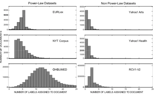
A second critical difference between large scale multi-label corpora and traditional benchmark datasets relates to the number of labels that are assigned to each document. Fig-ure2compares the distributions of the number of labels per document for the same corpora shown in Fig.1. The median number of labels per document for the real world, power-law style datasets are 6, 5, and 12 for EUR-Lex, NYT and OHSUMED, respectively. These numbers are significantly larger than those in the typical datasets used in multi-label classifi-cation experiments. For example, among the three benchmark datasets shown, the RCV1-v2 dataset has a median of 3 labels per document, and the Yahoo! Arts and Health datasets each have a median of only 1 label per document. These differences can significantly impact the performance of a classifier.
As the number of labels per document increases, it becomes more difficult for a discrim-inative algorithm to distinguish which words are discrimdiscrim-inative for a particular label. This problem is further compounded when there is little training data per label. For the purposes of illustration, consider the following extreme case: suppose that we are training a binary classifier for a label,c1, that has only been assigned to one document,d. Furthermore,
as-sume that two additional labels,c2andc3, have been assigned to documentd, and that these
labels occur in a relatively large number of documents. Since documentd is the only posi-tive training example for labelc1, an independent binary classifier trained onc1will learn a
discriminant function that emphasizes not only words from documentdthat are relevant to labelc1, but also words that are relevant to labelsc2andc3, since the classifier has no way
of “knowing” which words are relevant to these other labels. In other words, when training an independent binary classifier for labelc1, each additional label that co-occurs withc1will
introduce additional confounding features for the classifier, thereby reducing the quality of the classifier.
Note however that in the above example it should be relatively easy to learn which fea-tures are relevant to the labels c2 and c3, since these labels occur in a large number of
Fig. 2 Number of documents (y-axis) that haveLlabels (x-axis). The version of the NYT Annotated Corpus used in our experiments contains documents with 3 or more labels, hence the cutoff at 3
documents. Thus, we should be able to leverage this information to improve our classifier forc1by removing the features ind which we know to be relevant to these confounding
labels. One possible approach to address this problem is to learn which individual word to-kens within a document are likely to be associated with each label. If we could then use this information to identify which words withindare likely to be related toc2andc3, we
could “explain away” these words, and then use the remaining words for the purposes of learning a model forc1. Note that for this purpose it is useful to (1) remove the assumption
of label-wise independence, and (2) learn the models for all of the labels simultaneously, since learning which words within a document are irrelevant to a particular label is a key part of learning which words are relevant to the label.
1.2 A generative modeling approach
In a generative approach to document classification, one learns a model for the distribution of the words given each label, i.e., a model for P ( w|c),1≤c≤C, wherew is the set of words in a document, and constructs a discriminant function for the label via Bayes rule. In standard supervised learning, with one label per document, theseCdistributions are typically learned independently. With multi-label data, the distributions should instead be learned simultaneously since we cannot separate the training data intoCgroups by label.
A useful approach in this context is a model known as latent Dirichlet allocation (LDA) (Blei et al.2003), which we will also refer to as topic modeling, which models the words in a document as being generated by a mixture of topics, i.e.,P (w|d)=cP (w|c)P (c|d), whereP (w|d)is the marginal probability of wordwin documentd,P (w|c)is the probabil-ity of wordwbeing generated given labelc, andP (c|d)is the relative probability of each of theclabels associated with documentd. LDA has primarily been viewed as an unsupervised learning algorithm, but can also be used in a supervised context (e.g., Blei and McAuliffe 2008; Mimno and McCallum2008; Ramage et al. 2009). Using a supervised version of
LDA it is possible to learn both the word-label distributionsP (w|c)and the document-label weightsP (c|d)given a training corpus with multi-label data.
What is particularly relevant is that this approach (1) models the assignment of labels at the word-level, rather than at the document level as in discriminative models, and (2) learns a model for all labels at the same time, rather than treating each label independently. In partic-ular, for the documentdin our earlier example that was assigned the set of labels{c1, c2, c3},
the model can explain away words that belong to labelsc2andc3—i.e., words that have high
probabilityP (w|c)under these labels. Sincec2and c3are frequent labels, it will be
rela-tively easy to learn which features are relevant to these labels, since the confounding features introduced by co-occurring labels in a multi-label scheme will tend to cancel out over many documents. The remaining words that cannot be explained well byc2orc3will be assigned
to labelc1, and the model will learn to associate such words with this label and not associate
withc1the words that are more likely to belong to labelsc2andc3. This general intuition
is the basis for our approach in this paper. Specifically, we investigate supervised versions of topic models (LDA) as a general framework for multi-label document classification. In particular, the topic modeling approach allows for the type of “explaining away” effect at the word level that we hypothesize should be particularly helpful for the types of rare labels that pose challenges to purely discriminative methods.
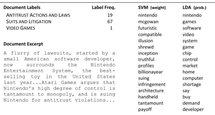
Figure3illustrates the advantages an LDA-based approach has in terms of learning rare labels. On the left is the partial text of a news article, taken from the New York Times, along with three human-assigned labels:ANTITRUST ACTIONS AND LAWSandSUITS AND LIT-IGATION(which both occur in multiple other documents) andVIDEO GAMES (for which this document is the only positive example in the training data). On the right are the words with the highest weights from a binary SVM classifier trained on the labelVIDEO GAMES. Beside this column are the highest probability words learned by an LDA-based model (de-scribed in more detail later in the paper). The words learned by the SVM classifier are quite noisy, containing a mixture of words relevant to the other two labels (e.g., suing,
infringe-ment, etc.), as well as rare words that are peculiar to the specific document rather than being
relevant features for any of the labels (e.g., futuristic, illusion, etc.). These words do not match our intuition of words that would be discriminative for the conceptVIDEO GAMES. Furthermore, as we will see later in the experimental results section, SVM classifiers trained on rare labels in this type of multi-label problem do not predict well on new test documents. While the set of words learned by LDA model is still somewhat noisy, it is nonetheless clear the model has done a better job in determining which words are relevant to the labelVIDEO GAMES, and which of the words should be associated with the other two labels (e.g., there are no words with high probability that directly relate to lawsuits). The model benefits from not assuming independence between the labels, as with binary SVMs, as well as from the “explaining away” effect.
Thus far we have focused our discussion on the issue of learning appropriate models for labels during training. An additional issue that arises as the number of total labels (as well as the number of labels per document) increases, is the importance of accounting for higher-order dependencies between labels at prediction time (i.e., when classifying a new document). For example, suppose that we are predicting which labels should be assigned to a test-document that contains the word steroids. In a large-scale dataset like the NYT corpus, this word is a high-probability feature among many different labels, such as MEDICINE AND HEALTH, BASEBALL, and BLACK MARKETS. The ambiguity in the assignment of this word to a specific label can often be resolved if we account for the other labels within the document; e.g., the word steroids is likely to be related to the label BASEBALLgiven that the label SUSPENSIONS,DISMISSALS AND RESIGNATIONSis also assigned to the document,
Fig. 3 High-weight and high probability words for the labelVIDEO GAMESlearned by an SVM classifier and an LDA model (respectively) from the a set of New York Times articles, in which the labelVIDEO GAMES
only appeared once (text from the article is shown on the left)
whereas it is more likely to be related to MEDICINE AND HEALTHgiven the presence of the label CANCER.
Given this motivation, an additional beneficial feature of the topic model—and proba-bilistic methods in general— is that it is relatively straightforward to model the label depen-dencies that are present in the training data (a feature that we will elaborate on later in the paper). Modeling label dependencies is widely acknowledged to be important for accurate classification in multi-label problems, yet has been problematic in the past for datasets with large numbers of labels, as summarized in Read et al. (2009):
The consensus view in the literature is that it is crucial to take into account label cor-relations during the classification process . . . . However as the size of the multi-label datasets grows, most methods struggle with the exponential growth in the number of possible correlations. Consequently these methods are able to be more accurate on small datasets, but are not as applicable to larger datasets.
Thus, the ability of probabilistic models to account for label dependencies is a strong mo-tivation for considering these types of approaches in large-scale multi-label classification settings.
1.3 Contributions and outline
In the context of the discussion above, this paper investigates the application of statistical topic modeling to the task of multi-label document classification, with an emphasis on cor-pora with large numbers of labels. We consider a set of three models based on the LDA framework. The first model, Flat-LDA, has been employed previously in various forms. Ad-ditionally, we present two new models: Prior-LDA, which introduces a novel approach to account for variations in label frequencies, and Dependency-LDA, which extends this ap-proach to account for the dependencies between the labels. We compare these three topic models to two variants of a popular discriminative approach (one-vs-all binary SVMs) on five datasets with widely contrasting statistics.
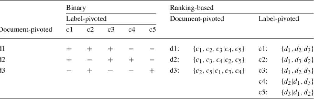
We evaluate the performance of these models on a variety of predictions tasks. Specifi-cally, we consider (1) document-based rankings (rank all labels according to their relevance to a test document) and binary predictions (make a strict yes/no classification about each label for a given document), and (2) label-based rankings (rank all documents according to their relevance to a label) and binary predictions (make a strict yes/no classification about each document for a given label).
The specific contributions of this paper are as follows:
– We describe two novel generative models for multi-label document classification, includ-ing one (Dependency-LDA) which significantly improves performance over simpler mod-els by accounting for label dependencies, and is highly competitive with popular discrim-inative approaches on large-scale datasets.
– We report extensive experimental results on two multi-label corpora with large numbers of labels as well as three smaller benchmark datasets, comparing the proposed genera-tive models with discriminagenera-tive SVMs. To our knowledge this is the first empirical study comparing generative and discriminative models on large-scale multi-label problems. – We demonstrate that LDA-based models—in particular the Dependency-LDA model—
can be highly competitive with, or better than, SVMs on large-scale datasets with power-law like statistics.
– For document-based predictions, we show that Dependency-LDA has a clear advantage over SVMs on large-scale datasets, and is competitive with SVMs on the smaller, bench-mark datasets.
– For label-based predictions, we demonstrate that Dependency-LDA generally outper-forms SVMs on large-scale datasets. We furthermore show that there is a clear perfor-mance advantage for the LDA-based methods on rare labels (e.g., labels with fewer than 10 training documents).
The remainder of the paper is organized as follows. We begin by describing how standard unsupervised LDA can be adapted to handle multi-labeled text documents, and describe our extensions that incorporate label frequencies and label dependencies. We then describe how inference is performed with these models, both for learning the model from training data and for making predictions on new test documents. An extensive set of experimental results are then presented on a wide range of prediction tasks on five multi-label corpora. We conclude the paper with a discussion of the relative merits of the LDA-based approaches vs. SVM-based approaches, particularly in the context of both the dataset statistics and prediction tasks being considered.
2 Related work
A number of approaches have been proposed for adapting the unsupervised LDA model to the case of supervised learning—such as the Supervised Topic Model (Blei and McAuliffe 2008), Semi-LDA (Wang et al.2007), DiscLDA (Lacoste-Julien et al.2008), and MedLDA (Zhu et al.2009)—however, these adaptations are designed for single label classification or regression, and are not directly applicable to multilabel classification.
A more recent approach proposed by Ramage et al. (2009)—Labeled-LDA (L-LDA)— was designed specifically for multi-label settings. In L-LDA, the training of the LDA model is adapted to account for multi-labeled corpora by putting “topics” in 1-1 correspondence with labels and then restricting the sampling of topics for each document to the set of labels that were assigned to the document, in a manner similar to the Author-Model described by
Rosen-Zvi et al. (2004) (where the set of authors for each document in the Author Model is now replaced by the set of labels in L-LDA). The primary focus of Ramage et al. (2009) was to illustrate that L-LDA has certain qualitative advantages over discriminative methods (e.g., the ability to label individual words, as well as providing interpretable snippets for document summarization). Their classification results indicate that under certain conditions LDA-based models may be able to achieve competitive performance with discriminative approaches such as SVMs.
Our work differs from that of Ramage et al. (2009) in two significant aspects. Firstly, we propose a more flexible set of LDA models for multi-label classification—including one model that takes into account prior label frequencies, and one that can additionally account for label dependencies—which lead to significant improvements in classification perfor-mance. The L-LDA model can be viewed as a special case of these models. Secondly, we conduct a much larger range and more systematic set of experiments, including in partic-ular datasets with large numbers of labels with skewed frequency-distributions, and show that generative models do particularly well in this regime compared to discriminative meth-ods. In contrast, Ramage et al. (2009) compared their L-LDA approach with discriminative models only on relatively small datasets (primarily on the Yahoo! sub-directory datasets discussed in the introduction).
Our work (as well as the Author Model and L-LDA model) can be seen as building on earlier ideas from the literature in probabilistic modeling for multilabel classification. McCallum (1999) and Ueda and Saito (2002) investigated mixture models similar to L-LDA, where each document is composed of a number of word distributions associated with document labels. These papers can be viewed as early forerunners of the more general LDA frameworks we propose in this paper.
More recently Ghamrawi and McCallum (2005) demonstrated that the probabilistic framework of conditional random fields showed promise for multilabel classification, com-pared to discriminative classifiers, as the number of labels within test documents increased. In follow-up work on these models, Druck et al. (2007) illustrated that this approach has the further benefit of being able to naturally incorporate unlabeled data for semi-supervised learning. A drawback of the CRF approach is scalability, particularly when accounting for label dependencies. Exact inference “is tractable only for about 3-12 [labels]” (Ghamrawi and McCallum2005). Alternatives to exact inference considered in Ghamrawi and McCal-lum (2005) include a “supported inference” method which learns only to classify the label combinations that occur in the training set, and a binary-pruning method that employs an intelligent pruning method which ignores dependencies between all but the most commonly observed pairs of labels. Although this method may improve upon approaches that ignore dependencies when restricted to datasets with few labels and many examples (such as tradi-tional benchmark datasets), it seems unlikely that any such methods will be able to properly account for dependencies in datasets with power-law frequency statistics (since nearly all dependencies in these datasets are between labels which have very sparse training data).
Zhang and Zhang (2010) present a hybrid generative-discriminative approach to multi-label classification. They first learn a Bayesian network structure that represents the inde-pendencies between labels. They then learn a discriminative classifier for each label in the order specified by the Bayesian network where the classifier for labelctakes as features not only the words in the document but also the output of the classifiers for each of the labels in the parent set ofc(i.e. the parent set specified by the Bayesian network). However, they apply their model to only small-scale datasets (the largest having 158 labels).
In terms of discriminative approaches to multi-label classification, there is a large body of prior work, which has been well-summarized elsewhere in the literature (e.g.,
see Tsoumakas and Katakis 2007; Tsoumakas et al. 2009). Most discriminative ap-proaches to multi-label classification have employed some variant of the “binary problem-transformation” technique, in which the multi-label classification problem is transformed into a set of binary-classification problems, each of which can then be solved using a suitable binary classifier (Rifkin and Klautau2004; Tsoumakas and Katakis2007; Tsoumakas et al. 2009; Read et al.2009). The most commonly employed method in the literature is the “one-vs-all” transformation, in whichCindependent binary classifiers are trained—one classifier for each label. These binary classification tasks are then handled using discriminative clas-sifiers, most notably SVMs, but also via other methods such as perceptrons, naive Bayes, and kNN classifiers. As our baseline discriminative method in this paper, we use the “one-vs-all” approach with SVMs as the binary classifier, since this is the most commonly used discriminative approach in the current multi-label classification literature, and has been de-fended in the literature in the face of an increasing number of proposed alternative methods (e.g., see Rifkin and Klautau2004). We note also that there is a prior thread of work on dis-criminative approaches that can handle label-dependencies. For example, another problem-transformation technique known as the “Label Powerset” method (Tsoumakas et al.2009; Read et al.2009) builds a binary classifier for each distinct subset of label-combinations that exist in the training data—however, these approaches tend not to scale well with large label sets due to combinatorial effects (Read et al.2009).
3 Topic models for multilabel documents
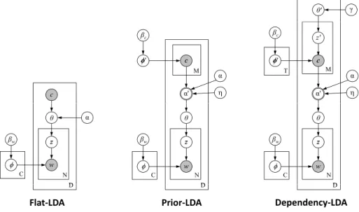
In this section, we describe three models (depicted in Fig.4using graphical model notation) that extend the techniques of topic modeling to multi-label document classification. Before providing the details for each model, we first briefly introduce the notation that will be used to describe these topic models within the multi-label inference setting, as well as provide a high-level description of the relationships between the three models.
The general setup of the inference task for the multi-label topic models we describe is as follows: the observed data for each document d∈ {1, . . . , D} are a set of words w(d)
and labels c(d). For all models, each label-typec∈ {1, . . . , C}is modeled as a multinomial
distributionφc over words. Each documentd is modeled as a multinomial distributionθd
over the document’s observed label-types. Words for document d are generated by first sampling a label-type z fromθd, and then sampling a word-tokenw fromφz. The three models that we present differ with respect to how they model the generative process for labels.
The first model we describe is a straightforward extension of LDA to labeled docu-ments, which we will refer to as Flat-LDA, where the labels are treated as given; this model makes no generative assumptions regarding how labels c(d)are generated for a document.
We then describe an extension to the Flat-LDA model—Prior-LDA—that incorporates a generative process for the labels themselves via a single corpus-wide multinomial distribu-tion over all the label-types in the corpus. This assumpdistribu-tion of Prior-LDA is very useful for making predictions when the label-frequencies are highly non-uniform. Lastly, we describe Dependency-LDA, which is a hierarchical extension to the previous two models that cap-tures the dependencies between the labels by modeling the generative process for labels via a topic model; in Dependency-LDA, label-tokens for each documentd are sampled from a set ofT corpus-wide topics, according to a document-specific distributionθd over the
topics. We note that the Flat-LDA and Prior-LDA models can be viewed as special cases of the LDA model. In particular, the Prior-LDA model is equivalent Dependency-LDA if we set the number of topicsT=1.
Fig. 4 Graphical models for multi-label documents. The observed data for each documentdare a set of words w(d)and labels c(d). Left: In Flat-LDA, no generative assumptions are made regarding how labels are generated; labels for each document are assumed to be given. Center: The Prior-LDA model assumes that the label-tokensc(d) for each document are generated by sampling from a corpus-wide multinomial distribution over label-typesφ, which captures the relative frequencies of different label-types across the corpus. Right: The Dependency-LDA model assumes that the label-tokens for each document are sampled from a set ofT corpus-wide topics—where each “topic”t corresponds to a multinomial distribution over label-typesφt—according to a document-specific distributionθd over these topics
3.1 Flat-LDA
The latent Dirichlet allocation (LDA) model, also referred to as the topic model, is an unsu-pervised learning technique for extracting thematic information, called topics, from a cor-pus. LDA represents topics as multinomial distributions over theW unique word-types in the corpus and represents documents as a mixture of topics. Flat-LDA is a straightforward extension of the LDA model to labeled documents. The set of LDA topics is substituted with the set of unique labels observed in the corpus. Additionally, each document’s distribution over topics is restricted to the set of observed labels for that document.
More formally, letCbe the number of unique labels in the corpus. Each labelcis repre-sented by aW-dimensional multinomial distributionφc over the vocabulary. For document
d, we observe both the words in the document w(d) as well as the document labels c(d).
The generative process for Flat-LDA is shown below. Each document is associated with a multinomial distributionθd over its set of labels. The random vectorθd is sampled from a symmetric Dirichlet distribution with hyper-parameterαand dimension equal to the number of labels|c(d)|. Given the distribution over topicsθ
d, generating the words in the document
follows the same process as LDA:
1. For each labelc∈ {1, . . . , C}, sample a distribution over word-typesφc∼Dirichlet(·|β) 2. For each documentd∈ {1, . . . , D}
(b) For each wordi∈ {1, . . . , NdW}
i. Sample a labelz(d)i ∼Multinomial(θd)
ii. Sample a wordw(d)i ∼Multinomial(φc)from the labelc=z(d)i
Note that this model assigns each word token within a document to just a single label— specifically to one of the labels that was assigned to the document. The model is depicted using graphical model notation in the left panel of Fig.4.
Due to the similarity between the Flat-LDA model presented here, and both the Author-Model from Rosen-Zvi et al. (2004) and the L-LDA model from Ramage et al. (2009), it is important to note precisely the relationships between these models. The Author-Model is conditioned on the set of authors in a document (and a “topic” is learned for each author in the corpus), whereas L-LDA and Flat-LDA are conditioned on the set of labels assigned to a document (and a “topic” is learned for each label in the corpus). L-LDA and Flat-LDA are in practice equivalent models, but employ different generative descriptions. Specifically, L-LDA models the generative process for each label in a document as a Bernoulli vari-able (where the parameter of the Bernoulli distribution is label-dependent). However, during training, estimating the Bernoulli parameters is independent from learning the assignment of words to labels (i.e. thezvariables). Thus, during training both L-LDA and Flat-LDA reduce to standard LDA with an additional restriction that words can only be assigned to the observed labels in the document. Similarly, when performing inference for unlabeled docu-ments (i.e. at test time), Ramage et al. (2009) assume that L-LDA reduces to standard LDA. In this way, both Flat-LDA and L-LDA are in practice equivalent despite L-LDA including a generative process for labels.1Due to the mismatch between the generative description of L-LDA and how it is employed in practice, we find it pedagogically useful to distinguish between the models presented here and L-LDA.
3.2 Prior-LDA
An obvious issue with Flat-LDA is that it does not account for differences in the relative frequencies of the labels within a corpus. This is not a problem during training, because all labels are observed for training documents. However, for the purpose of prediction (labeling new documents at test-time), accounting for the prior probabilities of each label becomes important, particularly when there are dramatic differences in the frequencies of labels in a corpus (as is the case with power-law datasets, as well as with many traditional datasets, such as RCV1-V2). In this section we present Prior-LDA, which extends Flat-LDA by in-corporating a generative process for labels that accounts for differences in the observed frequencies of different label types. This is achieved using a two-stage generative process for each document, in which we first sample a set of observed labels from a corpus-wide multinomial distribution, and then given these labels, generate the words in the document.
Letφ be a corpus-wide multinomial distribution over labels (reflecting, for example, a power-law distribution of label frequencies). For document d, we draw Md samples fromφ. Each sample can be thought of as a single vote for a particular label. We replace
α(d), the symmetric Dirichlet prior with hyperparameterα, with aC-dimensional vectorα(d)
where theith component is proportional to the total number of times labeli was sampled fromφ. Formally, the vectorα(d)is defined to be:
α(d)= η∗Nd,1 Md +α, η∗ Nd,2 Md +α, . . . , η∗ Nd,C Md +α (1)
1Due to equivalence of Flat-LDA and L-LDA in practice, the experimental results we present for Flat-LDA
whereNd,i is the number of times label i was sampled fromφ. In other words,α(d) is
a scaled, smoothed, normalized vector of label counts.2 The hyper-parameterη specifies the total weight contributed by the observed labels c(d) and the hyper-parameter α is an
additional smoothing parameter that contributes a flat pseudocount to each label. We define the document’s label set c(d)to be the set of labels with a non-zero component inα(d). To
make this model fully generative, we place a symmetric Dirichlet prior onφ.
Consider, for example, three labels {c1, c2, c3}with frequenciesφ= {0.5,0.3,0.2} in
the corpus. For documentd, we drawMd samples from φ. AssumeMd=5 and the set
{c1, c2, c1, c1, c1}was sampled. Then the hyper-parameterα(d)would be: α(d)= η∗4 5+α , η∗ 1 5+α , η∗ 0 5+α
If hyperparameter α=0, then α(d)has only two non-zero components (because the last component equals zero) and c(d)= {c1,c2}. In this case, the multinomial vectorθd drawn
from Dirichlet(α(d))will always have zero count for the third label (i.e. labelc3will have
probability zero in the document). Ifα >0, then c(d)= {c1,c2,c3}and labelc
3 will have
non-zero probability in the document. AsMd goes to infinity,α(d)approaches the vector
η φ+α.
The multinomial distribution may seem like an unnatural choice for a label-generating distribution since the observed labels in a document are most naturally represented using binary variables rather than counts. We experimented with alternative parameterizations such as a multivariate Bernoulli distribution. However, this introduced problems during both training and testing. As noted by Schneider (2004) in relation to modeling document
words (rather than labels), the multivariate Bernoulli distribution tends to overweight
nega-tive evidence (i.e. the absence of a word in a document) during training, due to the sparsity of the word-document matrix. This problem is compounded when modeling document
la-bels because there are considerably fewer lala-bels in a document than words. Furthermore, at
test time when the document labels are unobserved, a Bernoulli model will converge more slowly since the probability of turning on a label in a document is higher than the probability of turning off a label in a document (this is due to the fact that a label can only be turned off after all words assigned to that label have been assigned elsewhere).3
The generative process for the Prior-LDA model is:
1. Sample a multinomial distribution over labelsφ∼Dirichlet(·|βC)
2. For each labelc∈ {1, . . . , C}, sample a distribution over word-typesφc∼Dirichlet(·|βW)
3. For each documentd∈ {1, . . . , D}:
(a) SampleMdlabel tokensc(d)j ∼Multinomial(φ), 1≤j≤Md
(b) Compute the Dirichlet priorα(d)for documentdaccording to (1) (c) Sample a distribution over labelsθd∼Dirichlet(·|α(d))
(d) For each wordi∈ {1, . . . , NW d }
i. Sample a labelz(d)i ∼Multinomial(θd)
ii. Sample a wordw(d)i ∼Multinomial(φc)from the labelc=z(d)i
This model is depicted using graphical model notation in the center panel of Fig.4.
2In the training data, we setM
dequal to the number of observed labels in documentdandNd,iequal to 0
or 1 depending upon whether the label is present in the document.
3A related issue was the reason given by Ramage et al. (2009) for resorting in practice to a Flat-LDA scheme
3.3 Dependency-LDA
Prior-LDA accounts for the prior label frequencies observed in the training set, but it does not account for the dependencies between the labels, which is crucial when making predic-tions for new documents. In this section, we present Dependency-LDA, which extends Prior-LDA by incorporating another topic model to capture the dependencies between labels. The labels are generated via a topic model where each “topic” is a distribution over labels. Dependency-LDA is an extension of Prior-LDA in which there areT corpus-wide proba-bility distributions over labels, which capture the dependencies between the labels, rather than a single corpus-wide distribution that merely reflects relative label frequencies. We note that several models that represent or induce topic dependencies have been investigated in the past for unsupervised topic modeling (e.g., Blei and Lafferty2005; Teh et al.2004; Mimno et al.2007; Blei et al.2010). Although these models are related to varying degrees to the Dependency-LDA model, as unsupervised models they are not directly applicable to document classification.
Formally, letT be the total number of topics where each topict is a multinomial dis-tribution over labels denotedφt. Generating a set of labels for a document is analogous to generating a set of words in LDA. We first sample a distribution over topicsθd. To generate a single label we sample a topiczfromθd and then sample a label from the topicφz. We repeat this processMdtimes. As in Prior-LDA, we compute the hyper-parameter vectorα(d)
according to (1) and define the label set c(d)as the set of labels with a non-zero component.
Given the set of labels c(d), generating the words in the document follows the same process
as Prior-LDA.
1. For each topict∈ {1, . . . , T}, sample a distribution over labels,φt∼Dirichlet(βC)
2. For each labelc∈ {1, . . . , C}, sample a distribution over words,φc∼Dirichlet(βW)
3. For each documentd∈ {1, . . . , D}:
(a) Sample a distribution over topicsθd∼Dirichlet(γ )
(b) For each labelj∈ {1, . . . , Md}
i. Sample a topicz(d)j ∼Multinomial(θd)
ii. Sample a labelc(d)j ∼Multinomial(φt)from the topict=z(d)j
(c) Compute the Dirichlet priorα(d)for documentdaccording to (1) (d) Sample a distribution over labelsθd∼Dirichlet(·|α(d))
(e) For each wordi∈ {1, . . . , NW d }
i. Sample a labelz(d)i ∼Multinomial(θd)
ii. Sample a wordw(d)i ∼Multinomial(φc)from the labelc=z(d)i
The Dependency-LDA model is depicted using graphical model notation in the right panel of Fig.4.
3.4 Topic model inference methods—model training
This section gives an overview of the inference methods used with the three LDA-based models (Flat-LDA, Prior-LDA, and Dependency-LDA). We first describe how to perform inference and estimate the model parameters during training (i.e., when document labels are observed). We then describe how to perform inference for test documents (i.e., when labels are unobserved).
Training all three LDA-based models requires estimating theC multinomial distribu-tionsφc of labels over word-types. Additionally, Prior-LDA and Dependency-LDA require
estimation of the T multinomial distributionsφt of topics over label types, whereT =1 for Prior-LDA andT >1 for Dependency-LDA. Additionally, training (and testing) for all models requires setting several hyperparameter values.
Note that we set the hyperparameterα=0 in Prior-LDA and Dependency-LDA during training—but not during testing/prediction—which restricts the assignments of words to the set of observed labels for each document (see (1)). This is consistent with the assumptions of these models, because in the training corpus all labels are observed, and the models as-sume that words are generated by one of the true labels. This also greatly simplifies training, because it serves to decouple the upper and lower parts of the models (namely, withα=0, the topic-label distributionsφt and the label-word distributionsφc are conditionally
inde-pendent from each other, given that we have observed all labels).
Furthermore, estimation of the φc distributions is in fact equivalent for all three
mod-els whenα=0 for Prior-LDA and Dependency-LDA (and, for consistency, we used the same set of parameter estimates forφcwhen evaluating all models). A benefit—in terms of model evaluation—of using the same estimates forφc across all models is that it controls for one possible source of performance variability; i.e., it ensures that observed performance differences are due to factors other than estimation ofφc. Specifically, differences in model performance can be directly attributed to qualitative differences between the models in terms of how they parameterize the Dirichlet priorα(d)for each test document.
In addition to the smoothing parameter α, there are several other hyperparameters in the models that must be chosen by the experimenter. For all experiments, hyperparameters were chosen heuristically, and were not optimized with respect to any of our evaluation metrics. Thus, we would expect that at least a modest improvement in performance over the results presented in this paper could be obtained via hyperparameter optimization. For details regarding the hyperparameter values we used for all experiments in this paper, and a discussion regarding our choices for these values, see AppendixB.
3.4.1 Learning the label-word distributions:Φ
To learn theCmultinomial distributionsφcover words, we use a modified form of the
col-lapsed Gibbs sampler described by Griffiths and Steyvers (2004) for unsupervised LDA. In collapsed Gibbs sampling, we learn the distributionsφcover words, and theDdistributions
θdover labels, by sequentially updating the latent indicatorzi(d)variables for all word tokens in the training corpus (where theφc and θd multinomial distributions are integrated—i.e., “collapsed”—out of the update equations).
For Flat-LDA, the assignment of words in documentdis restricted to the set of observed labels c(d). For Prior-LDA and Dependency-LDA a word can be assigned to any label as long
as the smoothing parameterαis non-zero. The Gibbs sampling equation used to update the assignment of each word tokenz(d)i to a labelcis:
P (z(d)i =c|w(d)i =w,w−i,c(d),α(d),z−i, βW)∝ NW C wc,−i+βW W w=1(NwW Cc,−i+βW) ∗(Ncd,CD−i+α(d)c ) (2) whereNW C
wc is the number of times the wordwhas been assigned to the labelc(across the
entire training set), andNcdCDis the number of times the labelchas been assigned to a word
in documentd. We use a subscript−ito denote that the current token,zi, has been removed from these counts. The first term in (2) is the probability of wordw in labelc computed by integrating over theφcdistribution. The second term is proportional to the probability of labelcin documentd, computed by integrating over theθddistribution.
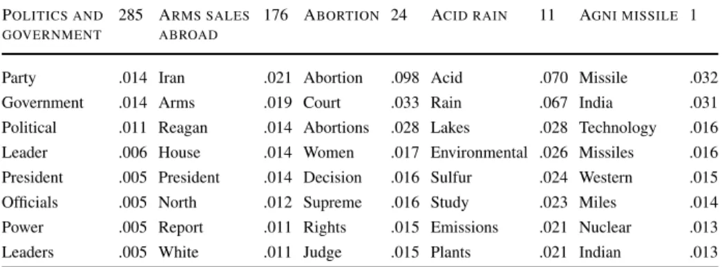
Table 1 The eight most likely words for five labels in the NYT Dataset, along with the word probabilities.
The number to the right of the labels indicates the number of training documents assigned the label POLITICS AND
GOVERNMENT
285 ARMS SALES ABROAD
176 ABORTION 24 ACID RAIN 11 AGNI MISSILE 1
Party .014 Iran .021 Abortion .098 Acid .070 Missile .032
Government .014 Arms .019 Court .033 Rain .067 India .031
Political .011 Reagan .014 Abortions .028 Lakes .028 Technology .016 Leader .006 House .014 Women .017 Environmental .026 Missiles .016 President .005 President .014 Decision .016 Sulfur .024 Western .015 Officials .005 North .012 Supreme .016 Study .023 Miles .014 Power .005 Report .011 Rights .015 Emissions .021 Nuclear .013 Leaders .005 White .011 Judge .015 Plants .021 Indian .013
For all results presented in this paper, during training we set α=0 andη equal to 50. Early experimentation indicated that the exact value ofηwas generally unimportant as long as η1. We ran multiple independent MCMC chains, and took a single sample at the end of each chain, where each sample consists of the current vector of z assignments (see AppendixBfor additional details). We use the z assignments to compute a point estimate of the distributions over words:
ˆ φw,c= NwcW C+βW W w=1(NwW Cc +βW) (3)
whereφw,cˆ is the estimated probability of wordw given labelc. The parameter estimates
ˆ
φw,c were then averaged over the samples from all chains. Several examples of label-word distributions, learned from a corpus of NYT documents, are presented in Table1.
Similarly, a point estimate of the posterior distribution over labelsθdfor each document is computed by: ˆ θc,d= N CD cd +α (d) c C c=1(NcCDd +α (d) c ) (4)
whereθc,dˆ is the estimated probability of labelcgiven documentd.
3.4.2 Learning the topic-label distributions:Φ
Note that this section only applies to the Prior-LDA and Dependency-LDA models since the Flat-LDA model does not employ a generative process for labels.4Learning theT multino-mial distributionsφtover labels is equivalent to applying a standard LDA model to the label
tokens. In our experiments, we employed a collapsed Gibbs sampler (Griffiths and Steyvers 2004) for unsupervised LDA, where the update equation for the latent topic indicatorszi(d)
4Additionally, since there is only one “topic” to learn for the Prior-LDA model, the estimation problem
for this model simplifies to computing a single maximum-a-posteriori estimate of the Dirichlet-multinomial distributionφ.
is given by: P (z(d)i =t|c (d) i =c, c−i,z’−i, γ , βC)∝ NCT ct,−i+βC C c=1(N CT ct,−i+βC) ∗Ndt,DT−i+γ (5) whereNCT
ct is the number of times labelc has been assigned to topict (across the entire
training set), andNDT
dt is the number of times topict has been assigned to a label in
doc-umentd. The subscript−i denotes that the current label-tokenzi has been removed from these counts. The first term in (5) is the probability of labelcin topictcomputed by inte-grating over theφtdistribution. The second term is proportional to the probability of topict
in documentd, computed by integrating over theθd distribution.
For training, we experimented with different values ofT ≤C (for Dependency-LDA). We set γ 1, and adjustedβC in proportion to the ratio of the number of topics T to
the total number of observed labels in each training corpus (see AppendixBfor additional details).
For each MCMC chain, we ran the Gibbs sampler for a burn-in of 500 iterations, and then took a single sample of the vector of zassignments. Given this vector, we compute a posterior estimate for theφtdistributions:
ˆ φc,t= N CT ct +βC C c=1(NcCTt +βC) (6)
whereφˆc,tis the estimated probability of labelcgiven topict. For each training corpus, we
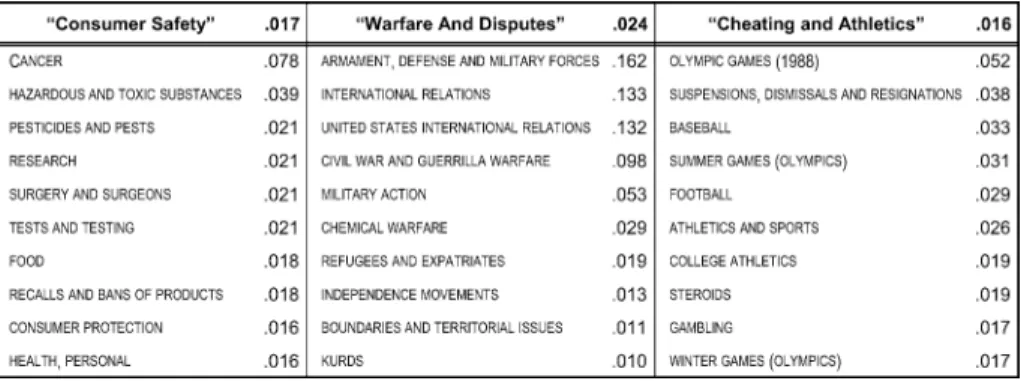
ran ten MCMC chains (giving us ten distinct sets of topics).5Several examples of topics, learned from a corpus of NYT documents, are presented in Table2.
Similarly, a point estimate of the posterior distribution over topicsθdfor each document
is computed by: ˆ θd,t= NDT dt +γ T t=1(NdDTt +γ ) (7)
whereθˆd,tis the estimated probability of topictgiven documentd.
3.5 Topic model inference methods—test documents
In this section, we first describe a proper inference method for sampling the three LDA-based models during test time, when the document labels are unobserved. In the following section, we describe an approximation to the proper inference method which is computa-tionally much faster, and achieved performance that was as accurate as the true sampling methods. We note again that the hyperparameter settings used for all experiments are pro-vided in AppendixB.
At test time, we fix the label-word distributions φcˆ, and topic-label distributions φˆt,
that were estimated during training. Inference for a test document d involves estimating its distribution over label typesθd and a set of label-tokens c(d), given the observed word
5We can not average our estimates ofφ
tover multiple chains as we did when estimatingφc. This because the
topics are being learned in an unsupervised manner, and do not have a fixed meaning between chains. Thus, each chain provides a distinct estimate of the set ofT φtdistributions. For test documents, we average our
Table 2 The ten most likely labels within three of the topics learned by the Dependency LDA model on the
NYT dataset. Topic labels (in quotes) are subjective interpretations provided by the authors
tokens w(d). Additionally, inference for Dependency-LDA involves estimating a document’s
distribution over topics, θd. We first describe inference at the word-label level (which is
equivalent for all three LDA models given the Dirichlet priorα(d)), and then describe the
additional inference steps involved in Dependency-LDA. Note that for all models, inference for each test document is independent.
The θd parameter is estimated by sequentially updating thez(d)i assignments of word
tokens to label types. The Gibbs update equation is modified from (2) to account for the fact that we are now using fixed values for theφcdistributions, which were learned during training, rather than an estimate computed from the current values of z assignments via
NW C wc : P z(d)i =c |w(d)i =w,w(d)−i, α(d), z(d)−i,φw,cˆ ∝ ˆφw,c∗ Ncd,CD−i+α (d) c (8)
whereφw,cˆ was estimated during training using (3),NCD
cd is the number of times the labelc
has been assigned to a word in documentd, and whereα(d)c is the value of the document-specific Dirichlet prior on label-typecfor documentd, as defined in (1).
The only difference that arises between the three LDA models when sampling the z variables is in the document-specific priorα(d). To simplify the following discussion, we describe inference in terms of Dependency-LDA. We note again that Prior-LDA is a special case of Dependency-LDA in whichT =1, and therefore the descriptions of inference for Dependency-LDA are fully applicable to Prior-LDA.6
Since the label tokens are unobserved for test documents, exact inference requires that we sample the label tokens c(d)for the document. The label tokens c(d)are dependent on the
assignment zof label-tokens to topics in addition to the vector of word-assignments z. We therefore must also sample the variablesz(d). The Gibbs sampling equation forc(d)i , given
the trained model, and a document’s vector ofzandzassignments, is:
p ci(d)=c|z(d)i =t, z−(d)i, c−(d)i, z(d),φˆt,c ∝ C c=1 (α (d) c +N CD c,d) C c=1 (α (d) c ) · ˆφt,c (9)
6In Flat-LDA, there is no document-specific Dirichlet prior. Instead, the prior for each document is simply a
symmetric Dirichlet with hyperparameterα, i.e. α(d)c =α, c∈1, . . . , C. Since this does not depend on any
where the first term on the right-hand side of the equation is the likelihood of the current vector of word assignments to labels z(d)given the proposed set of label-tokens c(d)(i.e.,
updated with valuec(d)i =c), andNcdCD is the total number of words in document d that
have been assigned to labelc. The second termφˆc,t was estimated during training using (6).
Since the update equation forc(d)i is not transparent from the model itself, and has not been presented elsewhere in the literature, we provide a derivation of (9) in AppendixC.
Given the current values of the label tokens c(d), the topic assignment variablesz(d)
are conditionally independent of the label assignment variablesz(d). The update equations
for thez(d) variables are therefore equivalent to (8), except that we are now updating the assignment of labels to topics rather than words to labels:
P z(d)i =t | ci(d)=c, γ , z(d)−i,φˆt,c ∝ ˆφc,t∗ Ndt,DT−i+γ (10) whereNDT
dt,−iis the number of times topicthas been assigned to a label in documentd, and
the document-specific distribution over topicsθdhas been integrated out.
For each test documentd, we sequentially update each of the values in the vectors z(d), c(d), and z(d)
. Since the z(d)variables are conditionally independent of the z(d)
variables given the c(d)variables, the c(d)variables are the means by which the word-level information
contained in z(d)and the topic-level information contained in z(d)
can propagate back and forth. Thus, a reasonable update order is as follows:
1. Update the assignment of the observed word tokensw(d)to the labels:z(d)(8)
2. Sample a new set of label-tokens:c(d)(9)
3. Update the assignment of the sampled label-tokens to one ofT topics:z(d)(10) 4. Sample a new set of label-tokens:c(d)(9)
Each full cycle of these updates provides a single ‘pass’ of information from the words up to the topics and back down again. Once the sampler has been sufficiently burned in, we can then use the vectors z(d), c(d)and z(d)to compute a point estimate of a test document’s
distributionθdˆ over the label types using (4) (and the prior as defined in (1)).
Unfortunately, the proper Gibbs sampler runs into problems with computational effi-ciency. Intuitively, the source of these problems is that thecvariables act as a bottleneck during inference since they are the only means by which information is propagated between the zand zvariables. To limit the extent of this bottleneck, we can increase the number of label tokens Md that we sample. However, this is computationally expensive because sampling eachcvalue requires substantially more computation than sampling thezandz
assignments, since computing each proposal value requires taking a product ofCgamma values.7
3.5.1 Fast inference for dependency-LDA
We now describe an efficient alternative to the sampling method described above. Experi-mentation with this alternative inference method suggests that, in addition to requiring sub-stantially less time, it in fact achieves similar or better prediction performance compared to proper inference.
7There are methods to optimize the sampler forc(d), which reduces the amount of computation required by
several orders of magnitude (using simplification of the expression in (9) and careful storage and updating of the vector of gamma values). However, this method was still slower by an order of magnitude per iteration than the ‘fast inference’ method presented in the following section, and required a much longer burn-in (while giving similar, or worse, prediction performance).
The idea behind the fast-inference method is that, rather than explicitly sampling the values ofc, we directly pass information between the label-level and topic-level parameters (thus avoiding the information bottleneck created by the ctokens, and also avoiding this costly inference step). This can be achieved by directly passing thezvalues up to the topic-level, and treating eachzvalue as if it was an observed label tokenc. In other words, we substitute the vector of sampled label tokensc(d)with the vector of label assignmentsz(d)
for each document; since bothz(d)i andc (d)
i can take on the same set of values (between 1
andC), these vectors can be treated equivalently when sampling the topic-assignmentsz(d)i
for them. Then, after updating thezvalues, we can directly compute the posterior predicted distribution over label types,p(c|d), by conditioning on the currentzassignments, and use this to computeα(d).
To motivate this approach, letΦbe the T-by-Cmatrix where rowt containsφt. Let θd be theT-dimensional multinomial distribution over topics. We can directly compute the posterior predictive distribution over labels givenΦandθd, as follows:
p(c(d)i =c|θd, Φ)∝ T t=1 p(c(d)i =c|z(d)i =t )·p(z (d) i =t|d) = T t=1 Φt,c ·θd,t (11)
Thus, given the matrixΦ(learned during training) and an estimate of theT-dimensional vectorθd, which we can compute using (7), the hyper-parameter vectorα(d)can be directly
computed using:
α(d)=η (θˆd·Φ)+α (12)
Once we have updated the z variables, (12) allows us to computeα(d) directly without
explicitly sampling thecvariables.8An alternative defense of this approach is that asMd goes to infinity in the generative model for Dependency-LDA, the vectorα(d)approaches
the expression given in (12).
The sequence of update steps we use for this approximate inference method is:
1. Update the assignment of the observed word tokensw(d) to one of theClabel types:
z(d)(8)
2. Set the label-tokens (c(d)) equal to the label assignments:c(d) i =z
(d) i
3. Update the assignment of the label tokens to one ofT topics:z(d)(10) 4. Compute the hyperparameter vector:α(d)(12)
As before, each full cycle of these updates provides a single ‘pass’ of information from the words up to the topics and back down again. But rather than sampling thec(d)
label-tokens, we directly pass thez(d)variables up to the topic-level sampler, and use these as an
approximation of the vectorc(d). Then, given the current estimate ofθ(d)(shown in (7)), we
compute theα(d)prior directly using (12).9
8This is in fact the correct posterior-predicted value ofα(d)in the generative model, given the variablesΦ andθd. However, technically this is not correct during inference, because it ignores the values of the z(d)
variables, which are accounted for in the first term in (9).
9Note that the computational steps involved in this method are in fact very close to the proper inference
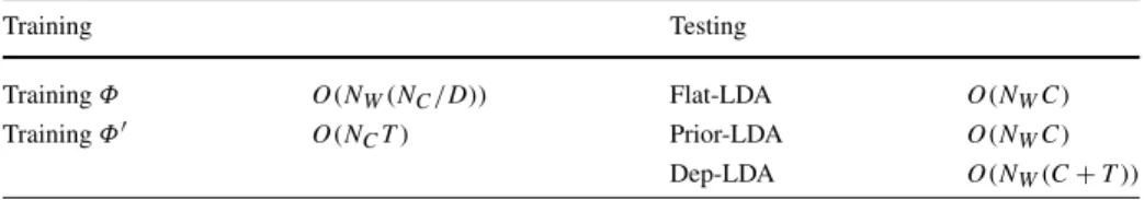
Table 3 Computational Complexity (per iteration) for the three LDA-based methods.NW: Number of
word-tokens in the dataset;NC: Number of observed label tokens in the (training) set;D: Number of documents in
the training set;C: Number of unique label-types;T: Number of topics
Training Testing
TrainingΦ O(NW(NC/D)) Flat-LDA O(NWC)
TrainingΦ O(NCT ) Prior-LDA O(NWC)
Dep-LDA O(NW(C+T ))
Once the sampler has been sufficiently burned in, we can then use the assignments z(d),
and z(d)to compute a point estimate of a test document’s distributionθˆdover the label types
using (4) (and the prior as defined in (12)).
We compared performance between this method and the proper inference method (with
Md=1000) on a single split of the EURLex corpus. In addition to providing significantly better predictions on the test dataset, the fast inference method was more efficient. Even after optimizing thec(d)i sampling, the fast inference method was well over an order of magnitude faster (per iteration) than proper inference, and also converged in fewer iterations. Due to its computational benefits, we employed the fast inference method for all experimental results presented in this paper.
The computational complexity for training and testing the three LDA-based algorithms is presented in Table3.10Note that the complexity of Dependency-LDA does not involve a term corresponding to the square of the number of unique labels (C), which is often the case for algorithms that incorporate label dependencies (a discussion of this issue can be found in, e.g., Read et al.2009).
3.6 Illustrative comparison of predictions across different models
To illustrate the differences between the three models, consider a word w that has equal probability under two labelsc1and c2(i.e.,φ1,w=φ2,w). In Flat-LDA, the Dirichlet prior
onθd is uninformative, so the only difference between the probabilities thatzwill take on value c1versus c2are due to the differences in the number of current assignments (NCD
forc1andc2) of word tokens in documentd. In Prior-LDA, the Dirichlet prior reflects the
relative a-priori label-probabilities (from the single corpus-wide topic), and therefore thez
assignment probabilities will reflect the baseline frequencies of the two labels in addition to the currentzcounts for this document. In Dependency-LDA, the Dirichlet prior reflects a prior distribution over labels given an (inferred) document-specific mixture of theT topics, and therefore the assignment probabilities reflect the relationships between the (inferred) document’s labels and all other labels, in addition to the current counts ofz.
Figure5shows an illustrative example of the predictions different models made for a single document in the NYT collection. An excerpt from this document is shown alongside the four true labels that were manually assigned by the NYT editors. The top ten label predictions (with the true labels in bold) illustrate how Dependency-LDA leverages both
step actually closely replicates what we would expect if we setMd=NdW and then sampled eachc (d) i
explicitly, except that we are now ignoring the topic-level information when we actually construct the vector
c(d)(although this information has a strong influence on thezassignments, so it is not unaccounted for in the
c(d)vector).