1
Conditional Betas, Higher Comoments and
the Cross-Section of Expected Stock Returns
by
Lei Xu
Submitted by Lei Xu, to the University of Exeter as a thesis for the degree of Doctor of Philosophy in Finance, June 2010.
This thesis is available for Library use on the understanding that it is copyright material and that no quotation from this thesis may be published without proper acknowledgement.
I certify that all material in this thesis which is not my own work has been identified and that no material has previously been submitted and approved for the award of a degree by this or any other University.
3
5
Acknowledgements
My deepest gratitude goes first and foremost to Professor Richard Harris, my supervisor, for his constant encouragement and guidance. He has walked me through all the stages of the writing of this thesis. Without his consistent and illuminating instruction, this thesis could not have reached its present form.
I would also like to acknowledge Dr. Cherif Guermet and Dr. Zhenxu Tong for very helpful instructions and Dr. Jian Shen for her help with data.
This thesis is dedicated to my parents. I would like to take this opportunity to say thank you to my beloved parents for their loving consideration and great confidence in me through all these years. Without your support and encouragement, I could not afford to come to the UK and finish my PhD and master’s degree in Exeter.
Special thanks go to Mrs. Kath Dugdale and Mr. Bernard Dugdale for providing me with accommodation and correcting the grammar of this thesis. I really enjoyed my time living with you.
I gratefully acknowledge the financial support from the Business School of the University of Exeter in the form of a graduate teaching assistantship. It gave me sufficient funding and valuable teaching experience.
7
Abstract
This thesis examines the performance of different models of conditional betas and higher comoments in the context of the cross-section of expected stock returns, both in-sample and out-of-sample.
I first examine the performance of different conditional market beta models by using monthly returns of the Fama-French 25 portfolios formed by the quintiles of size and book-to-market ratio in Chapter 3. This is a cross-sectional test of the conditional CAPM. The models examined include simple OLS regressions, the macroeconomic variables model, the state-space model, the multivariate GARCH model and the realized beta model. The results show that the state-space model performs best in-sample with significant betas and insignificant intercepts. For the out-of-sample performance, however, none of the models examined can explain returns of the 25 portfolios.
Next, I examine the recently proposed realized beta model, which is based on the realized volatility literature, by using individual stocks listed in the US market in Chapter 4. I extend the realized market beta model to betas of multi-factor asset pricing models. Models tested are the CAPM, the Fama-French three-factor model and a four-factor model including the three Fama-French factors and a momentum factor. Realized betas of different models are used in the cross-section regressions along with firm-level variables such as size, book-to-market ratio and past returns. The in-sample results show that market beta is significant and additional betas of multi-factor models can reduce although not eliminate the effects of firm-level variables. The out-of-sample results show that no betas are significant. The results are robust across different markets such as NYSE, AMEX and NASDAQ.
In Chapter 5, I test if realized coskewness and cokurtosis can help explain the cross-section of stock returns. I add coskewness and cokurtosis to the factor pricing models tested in Chapter 4. The results show that the coefficients of coskewness and cokurtosis have the correct sign as predicted by the higher-moment CAPM theory but only cokurtosis is significant. Cokurtosis is significant not only in-sample but also out-of-sample, suggesting
8
cokurtosis is an important risk. However, the effects of firm-level variables remain significant after higher moments are included, indicating a rejection of higher-moment asset pricing models. The results are also robust across different markets such as NYSE, AMEX and NASDAQ.
The overall results of this thesis indicate a rejection of the conditional asset pricing models. Models of systematic risks, i.e. betas and higher comoments, cannot explain the cross-section of expected stock returns.
9
Table of Contents
List of Tables and Figures... 13
Abbreviations ... 15 Chapter 1 Introduction ... 17 1.1 Background ... 17 1.2 Motivation ... 20 1.3 Contributions ... 21 1.4 Empirical results ... 23 1.5 Conclusion ... 24
1.6 Organization of this thesis ... 25
Chapter 2 Literature Review... 27
2.1 Mean-variance analysis and the CAPM ... 28
2.1.1 Mean-variance analysis ... 28
2.1.2 The Sharpe-Lintner CAPM ... 29
2.1.3 The conditional CAPM of Hansen and Richard ... 31
2.2 Empirical tests of the CAPM ... 33
2.2.1 Early empirical tests of the CAPM ... 34
2.2.2 Recent tests: the CAPM and the cross-section of expected returns ... 36
2.3 Explanations: what causes the failure of the CAPM? ... 38
2.3.1 The conditional CAPM ... 39
2.3.2 Multi-factor models ... 44
2.3.3 The higher-moment CAPM ... 46
2.3.4 Other explanations ... 47
2.4 Conclusion ... 49
Chapter 3 Conditional Market Beta and the Cross-Section of Stock Returns ... 51
3.1. Introduction ... 51
3.2. Empirical framework ... 55
10
3.2.2 The conditional CAPM and models of time-varying beta ... 56
3.2.2.1 The short-window regression ... 56
3.2.2.2 The macroeconomic variables model ... 57
3.2.2.3 The state-space model ... 58
3.2.2.4 The DCC-GARCH model ... 60
3.2.2.5 The realized beta model ... 62
3.2.3 The Fama-MacBeth approach ... 65
3.3. Data ... 66
3.3.1 Market and individual portfolio returns ... 66
3.3.2 Macroeconomic variables ... 67
3.3.3 Summary statistics ... 67
3.4 Empirical results ... 70
3.4.1 Estimation of conditional market beta models ... 70
3.4.1.1 The macroeconomic variables model ... 70
3.4.1.2 The state-space model ... 70
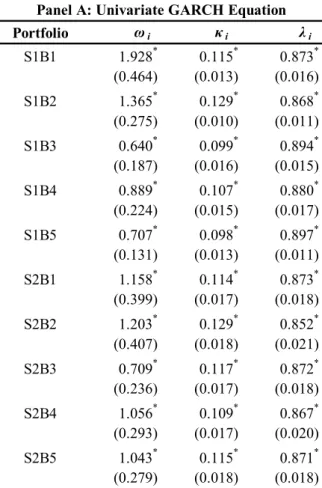
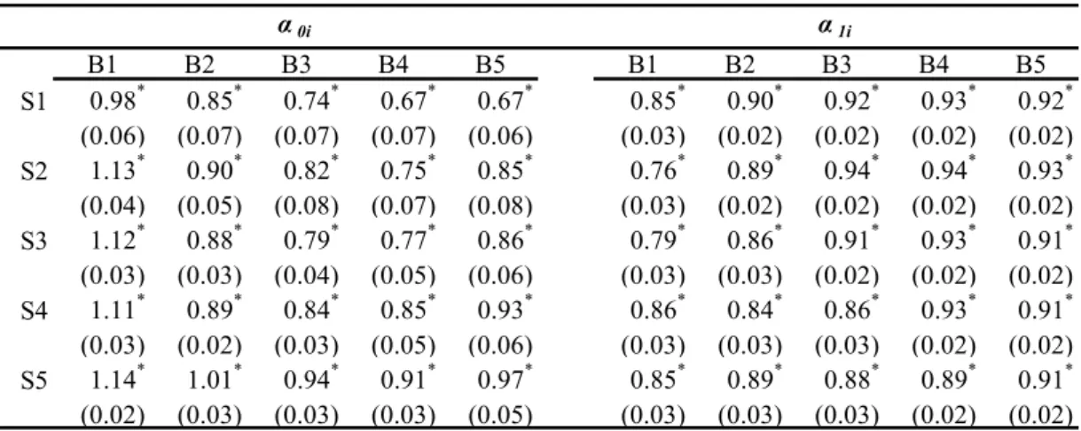
3.4.1.3 The DCC-GARCH(1,1) model ... 75
3.4.1.4 The realized beta model ... 75
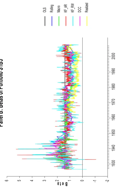
3.4.2 A comparison of the different models ... 75
3.4.3 Cross-sectional regression results ... 84
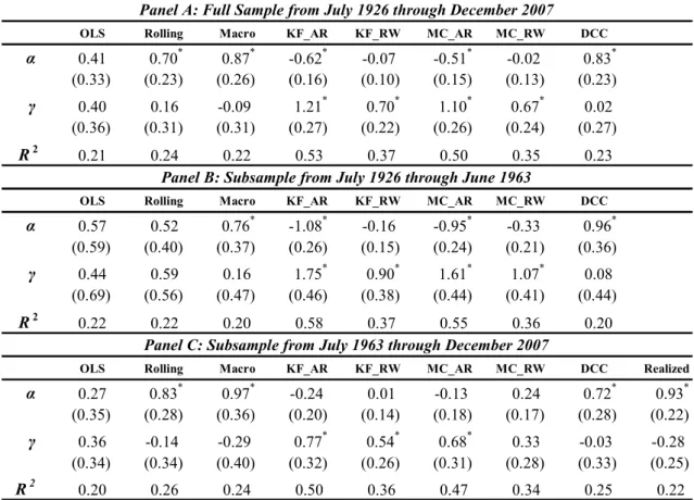
3.4.3.1 In-sample estimated market beta ... 84
3.4.3.2 Out-of-sample forecasted market beta ... 86
3.5 Conclusion ... 88
Appendix 3 ... 89
Chapter 4 Realized Betas and the Cross-Section of Stock Returns ... 97
4.1. Introduction ... 97
4.2. Factor pricing models and realized betas ... 101
4.2.1 Factor pricing models and measurement of realized betas ... 101
4.2.2 Modelling realized betas ... 105
11
4.3. Asset pricing models and factors ... 107
4.3.1 The CAPM ... 107
4.3.2 The Fama-French three-factor model ... 108
4.3.3 Fama-French model augmented by a momentum factor: a four-factor model ... 109
4.3.4 Summary ... 111
4.4. Data ... 111
4.5. Empirical results ... 113
4.5.1 Contemporaneously measured realized betas ... 115
4.5.2 In-sample forecasted realized betas ... 119
4.5.3 Out-of-sample forecasted betas... 122
4.6. Conclusion ... 125
Appendix 4: Robustness checks ... 127
Chapter 5 Can Higher Comoments Help Explain the Cross-Section of Stock Returns? ... 153
5.1 Introduction ... 153
5.2 The higher-moment CAPM ... 155
5.3 The estimation of higher comoments ... 159
5.4 Empirical results ... 161
5.4.1 Contemporaneous betas and higher comoments ... 161
5.4.2 In-sample forecasted betas and higher comoments ... 164
5.4.3 Out-of-sample forecasted betas and higher comoments ... 167
5.5 Conclusion ... 170
Appendix 5 ... 171
Chapter 6 Conclusion and Future Research ... 187
6.1 Conclusion ... 187
6.2 Future Research ... 189
13
List of Tables and Figures
Figure 2.1 Mean-Variance Analysis: Flexible and Efficient Set
Figure 2.2 The Capital Market Line (CML)
Table 3.1 Summary Statistics of Data
Table 3.2 Estimation Results of the Macroeconomic Variables Model
Table 3.3 Estimation Results of the State-Space Model
Table 3.4 Estimation Results of the DCC-GARCH model
Table 3.5 Estimation Results of the Realized Beta Model
Table 3.6 Comparison of the Unconditional and Conditional Betas
Table 3.7 Fama-MacBeth Cross-sectional Regression Results of in-sample Estimated Betas
Table 3.8 Fama-MacBeth Cross-sectional Regression Results of out-of-sample Forecasted Betas from Expanding Sample Method
Table A3.1 Fama-MacBeth Cross-sectional Regression Results of out-of-sample Forecasted Betas from Rolling Window Method
Figure 3.1 Plots of Betas
Table 4.1 Summary Statistics of Data
Table 4.2 Fama-MacBeth Regression Results with Contemporaneous Realized
Betas
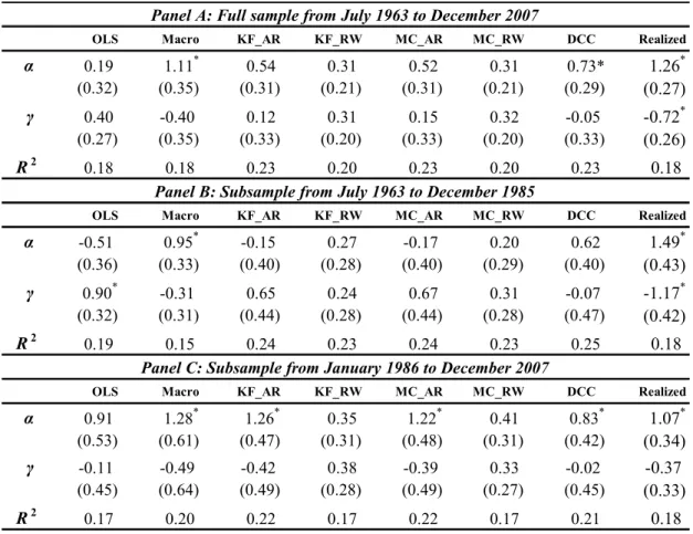
Table 4.3 Fama-MacBeth Regression Results with in-sample Forecasted Realized Betas
Table 4.4 Fama-MacBeth Regression Results with out-of-sample Forecasted Realized Betas
Table A4.1 Fama-MacBeth Regression Results with Alternative Measures of SIZE and Past Returns
Table A4.2 Fama-MacBeth Regression Results of Scholes and Williams (1977) Betas
Table A4.3 Fama-MacBeth Regression Results of Months Having at Least 20 Daily Returns
Table A4.4 Fama-MacBeth Regression Results of Quarterly Intervals
Table A4.5 Fama-MacBeth Regression Results with in-sample Forecasted Realized Betas from an AR(2) model
Table A4.6 Fama-MacBeth Regression Results with in-sample Forecasted Realized Betas from an AR(3) model
Table A4.7 Fama-MacBeth Regression Results with in-sample Forecasted Realized Betas from an ARMA(1,1) model
Table A4.8 Fama-MacBeth Regression Results with out-of-sample Forecasted Realized Betas from an AR(2) model
Table A4.9 Fama-MacBeth Regression Results with out-of-sample Forecasted Realized Betas from an AR(3) model
Chapter 3
Chapter 4 Chpater 2
14
Table A4.10 Fama-MacBeth Regression Results with out-of-sample Forecasted Realized Betas from an ARMA(1,1) model
Figure 4.1 Data Screening Process
Table 5.1 Fama-MacBeth Regression Results with Contemporaneous Realized
Betas and Higher Comoments
Table 5.2 Fama-MacBeth Regression Results with in-sample Forecasted Realized
Betas and Higher Comoments
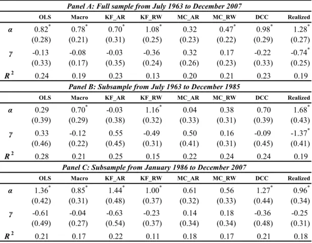
Table 5.3 Fama-MacBeth Regression Results with out-of-sample Forecasted
Realized Betas and Higher Comoments
Table A5.1 Fama-MacBeth Regression Results with in-sample Forecasted Realized
Betas and Higher Comoments from an AR(2) model
Table A5.2 Fama-MacBeth Regression Results with in-sample Forecasted Realized
Betas and Higher Comoments from an AR(3) model
Table A5.3 Fama-MacBeth Regression Results with in-sample Forecasted Realized
Betas and Higher Comoments from an ARMA(1,1) model
Table A5.4 Fama-MacBeth Regression Results with out-of-sample Forecasted
Realized Betas and Higher Comoments from an AR(2) model
Table A5.5 Fama-MacBeth Regression Results with out-of-sample Forecasted
Realized Betas and Higher Comoments from an AR(3) model
Table A5.6 Fama-MacBeth Regression Results with out-of-sample Forecasted
Realized Betas and Higher Comoments from an ARMA(1,1) model
15
Abbreviations
AMEX American Stock Exchange
APT Arbitrage Pricing Theory
AR Auto Regression
ARCH Auto Regressive Conditional Heteroskedasticity
ARMA Auto Regression Moving Average
BM Book-to-Market Ratio
CAPM Capital Asset Pricing Model
CAY Consumption-to-Wealth Ratio
CML Capital Market Line
CRSP The Centre for Research in Security Prices
D/E Debt-to-Equity Ratio
DCC Dynamic Conditional Correlation
FF3F Fama-French Three-Factor Model
GARCH Generalized Auto Regressive Conditional Heteroskedasticity
GDP Gross Domestic Product
GLS Generalized Least Squares
GMM Generalized Methods of Moments
ICAPM Intertemporal Capital Asset Pricing Model
MA Moving Average
MCMC Markov Chain Monte Carlo
NASDAQ National Association of Securities Dealers Automated Quotations
NYSE New York Stock Exchange
OLS Ordinary Least Squares
P/E Price-to-Earnings Ratio
17
Chapter 1
Introduction
1.1 Background
One of the central problems of finance is understanding the cross-section of asset returns. In academic research, it is at the centre of both theoretical and empirical studies of asset pricing models. In theoretical studies, a successful asset pricing model must be able to explain the cross-sectional patterns of returns of different assets. In empirical studies, the cross-section of returns has been explored in order to test theories and find interesting patterns for further theoretical research and practical use. In practice, investors also need to know what drives the different performances among assets when they make investments.
Although the first stock market was established more than 400 years ago (in Amsterdam in 1602), the first theory of the cross-section of returns was proposed only in the 1960s, the capital asset pricing model (CAPM) of Sharpe (1964) and Lintner (1965). In the CAPM, cross-sectional differences between returns are decided only by differences of systematic risk, called market beta. This conclusion is easy to understand because only systematic risk will be compensated and idiosyncratic risk will be diversified away in a well-diversified portfolio.
Early empirical tests of the CAPM focus on the relationship between returns and market beta. Researchers generally reject the model but find a positive coefficient of market beta in cross-sectional regressions (e.g. Black et al., 1972; Fama and MacBeth, 1973), indicating market beta is a priced risk although it alone cannot fully explain the cross-section of stock returns. Since the late 1970s, researchers have found other firm-level fundamental variables are also related to the cross-section of stock returns,
18
e.g. price-to-earnings ratio (Basu, 1977), size (Banz, 1981) and leverage (Bhandari, 1988). These findings indicate a rejection of the CAPM.
In 1992, Fama and French, in an influential study (Fama and French, 1992), comprehensively examine the cross-sectional relationship between stock returns, market beta and firm-level variables. They show that market beta is not priced but firm-level variables are significantly related to returns. Among firm-level variables, the combination of size and book-to-market ratio (BM) can drive out the explanatory abilities of other variables. Furthermore, Fama and French (1993, 1996) show that portfolios formed by size and BM are particularly challenging for the CAPM. They propose a new model with three factors related to the market, size and BM and show that the three-factor model can explain the returns of portfolios formed by different firm-level variables, except momentum portfolios. The studies of Fama and French have stimulated a rapidly expanding literature on the cross-section of stock returns.
Another important finding is the momentum effect of Jegadeesh and Titman (1993). They find that past returns within twelve months are positively correlated with future returns: past winners continue to be winners and past losers continue to be losers. The return differences between winners and losers cannot be explained by the CAPM or the Fama-French three-factor model. The momentum portfolios, along with the Fama-French size/BM portfolios, are among the most serious challenges to the CAPM.
Huge academic efforts have been devoted to explain the effects of size, BM and momentum. Within the asset pricing framework, there are three explanations: the conditional CAPM, multi-factor models and the higher-moment CAPM. At this point, I will briefly introduce the three categories, with details to follow in the next four chapters.
19
assumed to be constant. Hansen and Singleton (1982) prove that the conditional CAPM may hold even if the unconditional CAPM fails. In the conditional CAPM, conditional market beta is time-varying. Therefore, many researchers have tried to develop models for time-varying market beta. Widely used models in the literature include the popular rolling window estimation, the macroeconomic variables model (e.g. Shanken, 1990; Ferson and Harvey, 1999), the state-space model (e.g. Faff et al., 2000; Jostva and Philipov, 2004), the multivariate GARCH model (e.g. Braun et al., 1994; Bali, 2008) and the recently proposed realized beta model (Anderson et al., 2005, 2006).
The market return is the single risk factor generating returns of individual assets in the CAPM. Some researchers attribute the failure of the CAPM to the fact that the market return alone is not enough to explain asset returns so that other risk factors should be included. Theoretical frameworks include the intertemporal CAPM (ICAPM) of Merton (1973) and the arbitrage pricing theory (APT) of Ross (1974). However, the theory of multi-factor models does not give factors explicitly so that researchers must find them from empirical studies. Early studies use macroeconomic variables as factors (e.g. Chen et al., 1986). Recently, due to the success of explaining the cross-section of stock returns, models based on empirical findings of firm-level variables have become popular such as the Fama-French three-factor model (Fama and French, 1996) and Carhart’s four-factor model (Carhart, 1997). Subsequent studies put multi-factor models into a conditional framework so that multi-factor betas are also time-varying (e.g. Ferson and Harvey, 1999; Wang, 2003).
The CAPM is developed based on the mean-variance analysis of Markowitz (1952) where investors are assumed to care only about the mean and variance of returns. If returns do not follow an elliptical distribution and investors care about higher moments, such as skewness and kurtosis, then higher moments will be priced. This intuition has led to the development of the higher-moment CAPM. Kraus and Litzenberger (1976) propose a three-moment CAPM where coskewness is added into the traditional CAPM.
20
Fang and Lai (1997) extend this model to the four-moment CAPM. More recently, the conditional higher-moment CAPM has achieved some success in explaining the cross-section of stock returns. Harvey and Siddique (1999) and Smith (2007) find conditional coskewness is important; Dittmar (2002) proposes a conditional four-moment CAPM and finds that it cannot be rejected by using industry portfolios.
In modern finance, the cross-section of asset returns remains at the centre of finance research. New patterns have been found and existing patterns have been refined1; new models have been proposed and tested. In practice, practitioners, such as portfolio managers, pay close attention to academic findings in the cross-section of stock returns so that they can gain more guidelines in their investments. Overall, the cross-section of stock returns is one of the central problems in both academia and practice.
1.2 Motivation
The existing literature on testing conditional asset pricing models mainly focuses on their in-sample performance. For example, in tests of the conditional CAPM, Lettau and Ludvigson (2001) propose using the consumption-to-wealth ratio (CAY) to model market beta and find this variable is useful in explaining size/value portfolios in-sample; Jostova and Philipov (2004) propose the stochastic beta model, which is actually a state-space model estimated by the Markov chain Monte Carlo (MCMC) method, and test its in-sample cross-sectional performance by using individual stocks; Bali (2008) uses a bivariate GARCH model for the conditional beta and this study is also in-sample.
In the context of multi-factor models and the higher-moment CAPM, many studies also focus on in-sample performance. The original three-factor model of Fama and French (1996) is proposed and tested in an unconditional form. Subsequent tests of its conditional version focus on its in-sample performance such as He et al. (1996). For the
21
higher-moment CAPM, due to the difficulties of modelling coskewness and cokurtosis, most studies also focus on in-sample performance such as Kim (1987), Ditmmar (2002) and Smith (2007).
However, a true test of conditional asset pricing models should be an out-of-sample test. In the theoretical setting of conditional asset pricing models, investors only use information available when they make investment decisions. Using the full sample to estimate models inevitably utilises information beyond investors’ information set and therefore can lead to some bias, such as the over-conditioning bias studied by Boguth et al. (2008). In practice, it could be misleading if investors make decisions based on the in-sample performance of a model because a model’s out-of-sample performance may be substantially different from its in-sample performance.
Based on the considerations above, I examine whether different conditional models can explain the cross-section of stock returns not only in-sample but also out-of-sample. In out-of-sample tests, I use information only available at time period t to estimate the model and then use estimated parameters to forecast betas or higher comoments of time period t+1. The one-step-ahead forecasted betas or higher comoments are used in the cross-sectional regressions. In this way, I can test if a conditional model can truly explain the cross-section of stock returns out-of-sample. This is more relevant to conditional asset pricing models both in academic theory and in practice.
1.3 Contributions
The first contribution of the thesis is the examination of the out-of-sample performance of different conditional asset pricing models. As discussed in the last section, out-of-sample tests of conditional asset pricing models are more important than in-sample tests but many studies focus only on in-sample tests.
22
Some existing studies do use out-of-sample cross-sectional tests of conditional models but they mainly restrict their techniques to the rolling window OLS regressions. For example, the study by Avramov and Chordia (2006) uses a 36-month rolling window to estimate their models. Researchers who propose more advanced techniques usually only examine in-sample performance such as the studies cited in the last section (e.g. Jostova and Philipov, 2004; Bali, 2008).
The second contribution of the thesis is the examination of the performance of the recently proposed realized beta model in the cross-section of stock returns by using both portfolios and individual stocks listed in the US market, both in-sample and out-of-sample. Realized beta (Andersen et al., 2005, 2006) is based on the recent literature of realized volatility (Andersen et al., 2003; Barndorff-Nielson and Shephard, 2004). Andersen et al. (2005) study the time series properties of realized market beta of the Fama-French 25 portfolios and Morana (2009) tests the in-sample cross-sectional relationship between realized multi-factor betas and returns of those 25 portfolios. Andersen et al. (2006) study the properties of realized market beta of the 30 stocks in the Dow Jones Industrial Index (DJIA). However, no studies have examined the out-of-sample relationship between realized betas and returns. In this thesis, I first examine the out-of-sample relationship between forecasted realized market beta and returns of the Fama-French 25 portfolios. Then, I examine both in-sample and out-of-sample relationships between realized betas and individual stock returns by using all the stocks listed in the US market (NYSE, AMEX and NASDAQ). I also extend the realized single-factor market beta to multi-factor betas. This is the first study to examine comprehensively the relationships between realized betas and returns by using such a large universe of stocks.
The third contribution of the thesis is to extend the realized beta model to the measurement of higher comoments. Based on the realized beta model, I use high frequency returns to compute low frequency coskewness and cokurtosis and then
23
examine the relationship between returns and higher comoments both in-sample and out-of-sample. The method of computing higher comoments is simpler than many techniques used in current literature (e.g. Harvey and Siddique, 1999). The test assets are also stocks listed in the US market.
1.4 Empirical results
The overall results show that some conditional beta models, such as the state-space model for the Fama-French 25 portfolios and the realized beta model for individual stocks, can explain part of the effects of size, value and momentum in-sample but none of the models examined can explain those effects out-of-sample.
In Chapter 3, I examine different conditional market beta models of the conditional CAPM by using monthly returns of the Fama-French 25 portfolios. The models include simple OLS regression, the macroeconomic variables model, the state-space model, the multivariate GARCH model and the realized beta model. The monthly portfolio returns are regressed on each of those betas in the cross-section. In-sample, the state-space model performs very well in the sense of a significant beta, an insignificant alpha and a high value of R-squared. Out-of-sample, however, none of the models examined can generate a significantly priced conditional beta. The results are robust across different subsamples and estimation intervals.
In Chapter 4, the recently proposed realized beta model is tested using individual stocks in the US market. I use daily returns within each month to estimate betas of different factor pricing models. The models considered are the CAPM, the Fama-French three-factor model and a four-factor model, which is the Fama-French three-factor model augmented by a momentum factor. Betas used in the cross-sectional regressions are contemporaneously measured betas, in-sample forecasted betas and out-of-sample forecasted betas. For contemporaneously measured betas, betas of the market, size
24
factor (SMB) and momentum factor (WML) are significant while beta of the value factor (HML) is insignificant; the inclusion of betas of additional factors besides the market return does reduce the effects of size, BM and momentum although it does not eliminate those effects. For in-sample forecasted betas, betas of the market and WML remain significant but betas of SMB and HML are not. For out-of-sample forecasted betas, no betas are significantly priced. My results show that in-sample and out-of-sample forecasted betas can have very different performance. Testing a model only based on its in-sample performance may lead to the wrong conclusion. For example, Bali et al. (2009) find a significantly positive risk premium of in-sample forecasted realized market beta. My results, in contrast, show that out-of-sample forecasted realized market beta has a negative coefficient.
In Chapter 5, I extend the method of realized beta to estimate coskewness and cokurtosis. I add coskewness and cokurtosis into the cross-section regressions to examine if they can help explain the cross-section of stock returns. Similar to Chapter 4, I use contemporaneously measured, in-sample forecasted and out-of-sample forecasted coskewness and cokurtosis. The coefficients of both contemporaneously measured coskewness and cokurtosis have the correct signs but only cokurtosis is significant. Cokurtosis is an important risk because it is significant both in-sample and out-of-sample which is consistent with existing evidence of leptokurtosis of stock returns. Coskewness, however, is insignificant both in-sample and out-of-sample.
1.5 Conclusion
The unconditional CAPM cannot explain the effects of firm-level variables on the cross-section of stock returns. Academic efforts have been devoted to explain the failure of the unconditional CAPM. The explanations within the asset pricing framework include the conditional CAPM, multi-factor models and the higher-moment CAPM. In modern finance, multi-factor models and the higher-moment CAPM are also put in a
25
conditional framework. Therefore, tests of those models focus on their conditional performance. Specifically, the question is whether conditional betas and higher comoments can explain the cross-section of stock returns.
This thesis examines different techniques of conditional betas and higher comoments. The main focus is on the comparison of in-sample and out-of-sample performance of those techniques. In in-sample analysis, the state-space model is the best model for the Fama-French 25 portfolios and realized betas and higher comoments are significant for individual stocks except beta of HML and coskewness. Out-of-sample, however, none of the models examined can generate significant betas or higher comoments. The only exception is that out-of-sample forecasted cokurtosis is significant. The results of this thesis indicate a rejection of conditional asset pricing models.
The results of the thesis cast some doubt on testing conditional asset pricing models based on their in-sample performance, which is the focus of many previous studies. This thesis shows that the results of out-of-sample forecasted betas can be substantially different from in-sample estimated betas. Betas significant in-sample will not necessarily be significant out-of-sample because the success of models’ in-sample performance may be subject to over conditioning and over fitting bias. Furthermore, it may be misleading if we make judgements based on a model’s in-sample performance. Therefore, it is important to test a model not only based on its in-sample performance but also out-of-sample performance.
1.6 Organization of this thesis
The remainder of this thesis is organized as follows. In Chapter 2, I review comprehensively the literature on the cross-section of expected returns within an asset pricing framework. Other explanations such as behavioural finance are also mentioned briefly to give readers a complete picture of this area.
26
In Chapter 3, I test different conditional market beta models by using the Fama-French 25 size/value portfolios. The state-space model performs best in-sample with insignificant intercepts and significant market beta, which is consistent with existing literature. None of the models, however, can explain the cross-section of returns of the 25 portfolios out-of-sample. The results indicate a rejection of the conditional CAPM.
Chapter 4 tests the conditional CAPM and multi-factor models using the recently proposed realized beta model. Test assets are individual stocks listed in the US market. The results show that betas of the market, size factor and momentum factor are significant in-sample but insignificant out-of-sample. Furthermore, betas cannot fully explain the effects of firm-level variables.
Chapter 5 adds realized coskewness and cokurtosis to the factor pricing models tested in Chapter 4 to test whether higher comoments are priced and can help explain the cross-section of stock returns. The results show that cokurtosis is a significant risk both in-sample and out-of-sample, which is consistent with the evidence on the leptokurtosis of returns’ distributions. Coskewness, however, is insignificant. Adding coskewness and cokurtosis to factor pricing models cannot help explain the cross-section of stock returns.
The last chapter, Chapter 6, makes conclusions of the thesis and gives future research directions.
27
Chapter 2
Literature Review
In this chapter, I review the literature on the cross-section of stock returns within the asset pricing framework. Understanding the cross-section of stock returns has long been the centre of finance in both academia and practice, i.e. why different stocks have different expected returns. The capital asset pricing model (CAPM) of Sharpe (1964) and Lintner (1965), which is based on the mean-variance framework of Markowitz (1952, 1959), states that the cross-section of returns is only decided by differences in stocks’ systematic risk, market beta. Early empirical tests of the CAPM by Black et al. (1972) and Fama and MacBeth (1973) find there is a positive relationship between market beta and returns but this relationship is too flat. Since the 1980s, however, researchers have found that the cross-section of stock returns is related to firm-level variables such as P/E (Basu, 1977), size (Banz, 1981), and book-to-market ratio (BM) (Fama and French, 1992). Fama and French (1992) comprehensively study the relationship between returns, market beta and firm-level variables. They show that market beta is not priced but firm-level variables such as size and BM are significant. This is among the most serious challenges of the CAPM. Subsequent research has been focused on the explanation of those anomalies. Within the asset pricing framework, there are three major approaches. The first is the conditional CAPM which focuses on the time-varying property of market beta. The second is the multi-factor model such as Fama and French (1993) which uses other factors to explain the cross-section of stock returns. The third is the higher moment CAPM which adds coskewness and cokurtosis into the CAPM (e.g. Kraus and Litzenberger, 1976).
Based on the brief introduction above, the following review will start with the mean-variance analysis and the CAPM because the CAPM is the first asset pricing model and is still used as a benchmark model in both academia and practice. Furthermore, all the anomalies are actually abnormal returns under the CAPM. Then, I
28
will give a brief review of the abnormal returns associated with different firm-level variables with focus on size, BM and past returns. A lot of research has been devoted to explaining those abnormal returns. I focus on the explanation within the asset pricing framework under the assumption of rational investors. Specifically, I give a detailed review of the conditional CAPM, multi-factor models and the higher-moment CAPM. Of course, there are other explanations such as irrational investors within the behavioural finance framework and the effects of market microstructure. However, the focus of this thesis is on asset pricing in a rational expectations framework and so I will only give a brief review of the other explanations. Asset pricing models can also be expressed in discount factor form (e.g. Cochrane, 2001) but the techniques for conditional betas cannot enter the discount factor easily, so I will only mention the discount factor models when necessary.
2.1 Mean-variance analysis and the CAPM
2.1.1 Mean-variance analysis
There has been a long history of dealing with risk in financial markets. The first stock market can be tracked back to 1602 when shares of the East India Company began trading in Amsterdam (Perold, 2004). However, the theoretical foundation of decision making under uncertainty was developed only from the 1940s. Von Neumann and Morgenstern (1944) develop the utility function of payoff and uncertainty and formally state the trade-off between risk and return.
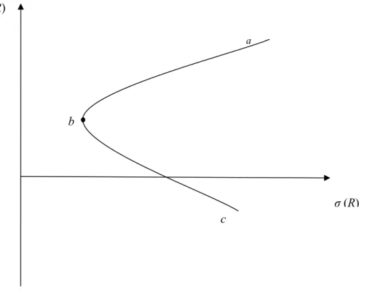
Markowitz (1952, 1959) puts the risk-return trade-off in a portfolio framework and formally uses variance as a measure of risk. The assumptions of Markowitz’s model include that investors are risk averse and only care about the mean and variance of portfolios for one period. Under those assumptions, investors will choose mean-variance efficient portfolios which minimize the variance for a given expected return or maximize expected return for a given variance. Figure 2.1 graphs the possible
29
investment opportunities for investors. The curve abc and the area within it are all investment opportunities but only the curve above point b, which is the global minimum variance portfolios (GMVP), is the efficient set, also called the efficient frontier. Therefore, investors will only choose portfolios on the curve from b to a based on their utility functions.
2.1.2 The Sharpe-Lintner CAPM
Built on the mean-variance analysis of Markovitz, Sharpe (1964) and Lintner (1965) propose the CAPM by adding additional assumptions. First, investors have identical expectations of the distribution of asset returns. The second is that all investors can borrow and lend any amount at the same risk free rate. The last one is that the market is in equilibrium and is complete with no frictions. Under those additional assumptions,
Figure 2.1 Mean-Variance Analysis: Flexible and Efficient Set
The figure plots the flexible and efficient set of the mean and variance analysis of Markowitz. E(R) is the expected return and σ(R) is the standard deviation of returns. Point b denotes the global minimum variance portfolios (GMVP). The curve abc and the area within are the flexible set but only the curve above b is efficient in the sense that lower standard deviations for a given return or higher returns for a given standard deviation. The curve above b is called efficient set or efficient frontier.
a
b
c E(R)
30
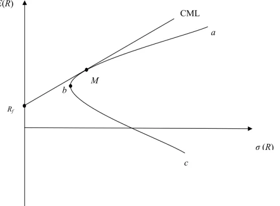
investors will choose the same risky assets and therefore these risky assets form the market portfolio. The efficient frontier now becomes the tangent line of the efficient frontier with only risky assets from the risk free rate, which is called the capital market line (CML). The graph of CML is in Figure 2.2. The efficient frontier is the tangent line crossing Rf and M, which is the market portfolio. Different investors will invest
different weights in the risk free asset and the market portfolio but they will hold the same risky asset portfolio, i.e. the market. The CAPM also implies that the market portfolio is efficient. For individual assets, the CAPM implies the following relationship,
( )
i f i(
( M) f)
, 1,...,E R =R +β E R −R i= N (2.1)
where βi is called market beta and defined as
Figure 2.2 The Capital Market Line (CML)
The figure plots the capital market line of Sharpe (1964) and Lintner (1965). E(R) is the expected return and σ(R) is the standard deviation of returns. Rf is the risk free rate. Point b denotes the global
minimum variance portfolios (GMVP) and the curve abc and the area within are the flexible set when there are only risky assets. M denotes the market portfolio, which is the tangent point from Rf. The
straight line from Rf and M is the new efficient frontier when there is a risk free asset.
M a b c E(R) σ (R) Rf CML
31 ( ( ) , ) i M i M R Cov R Var R β = . (2.2)
According to the CAPM, asset returns are decided only by their market beta, the systematic risk. Therefore, the cross-sectional differences of asset returns are only attributed to the cross-sectional differences of market beta:
( )i i
E r =λβ (2.3)
where ri is the excess return of asset i. The risk premium, λ, should be positive, so
assets with high betas should have higher returns than those with low betas.
Black (1972) relaxes the assumption that there is a risk free asset. He proves that the market portfolio is still efficient if unrestricted short sales are allowed. But the risk free rate in equation (2.1) is replaced by the return of a zero-beta portfolio. Of course, the assumption of unrestricted short sales is unrealistic but the market portfolio is no longer efficient without this assumption.
2.1.3 The conditional CAPM of Hansen and Richard (1987)
The Sharpe-Lintner CAPM states the relationship between unconditional expected return and beta. Using unconditional expectations omits conditioning information used by investors when they make decisions. Information accumulates over time and investors update their expectations when new information arrives, which in turn will result in new portfolio choices. Therefore, asset pricing models should incorporate the conditional expectations of investors.
Hansen and Richard (1987) study the conditional portfolio choice problem of investors. They solved both the unconditional and conditional mean-variance optimization
32
problems. The unconditional optimization is to minimize the unconditional portfolio variance for given unconditional expected returns,
Minww w′Σ s t. . w E′ =
µ
;w′ι
=1, (2.4)where w is a vector of weights of individual assets, ι is a vector of 1, E and ∑ are mean and variance/covariance matrix of returns, respectively. The conditional optimization is to minimize the conditional portfolio variance for given conditional expected returns,
Minww′Σtw s t. . w E′ t =
µ
;w′ι
=1 (2.5)where Et and ∑t are the conditional mean and variance/covariance matrix of returns,
respectively. Hansen and Richard find that the solution of the conditional optimization is different from the unconditional optimization.2
Furthermore, they prove that a portfolio on the conditional frontier may not be on the unconditional frontier. Therefore, the CAPM may hold conditionally even if it fails unconditionally. The conditional CAPM is
(
)
, 1 , , 1 ( ) ( ) t i t f i t t M t f E R + =r +β E R + −r , (2.6) where , 1 , 1 , , 1 ( , | ) ( | ) i r m t t i t m t t Cov r r I Var r Iβ
+ + + = . (2.7)The conditional CAPM states the relationship between conditional expected returns and
33
beta, which is the conditional counterpart of the Sharpe-Lintner CAPM.
2.2 Empirical tests of the CAPM
In this subsection, I focus on the cross-sectional tests of the CAPM which test the two implications from equation (2.3): the first is that market beta can fully explain the cross-section of asset returns and no other variables have marginal explanatory abilities and the second is that market beta has a positive risk premium. Of course, there are other approaches of testing the CAPM such as testing the efficiency of the market portfolio and time series tests of zero intercepts. My thesis focuses on the cross-section of stock returns, betas and firm-level variables so I mainly review the literature of cross-sectional tests and mention other approaches only when necessary.
Before summarizing the empirical results, it is necessary to highlight the difficulties inherent in empirical tests of the CAPM. The first is the well-known critique of Roll (1977) that the CAPM is untestable because the true market portfolio is unobservable. In empirical tests, researchers often use an index of a broad market such as the CRSP index of the US market as a proxy for the true market portfolio. Second, market beta is also unobservable. Therefore, only estimates of the true beta are used in the cross-section regressions, which cause the error-in-variables problem and can distort the estimate of the market risk premium. To overcome this problem, one can adjust the errors in estimated betas directly (e.g. Kim, 1996). A more common approach is to sort stocks into portfolios according to their betas or other variables such as size and BM because a diversified portfolio’s beta can be estimated more accurately than individual assets’ beta. However, sorting stocks into portfolios suffers from the well-known data snooping bias (Lo and MacKinlay, 1990). Therefore, more recent tests also attempt to use individual stocks as test assets and try to mitigate the error-in-variables problem at the same time (e.g. Brennan et al., 1998).
34
2.2.1 Early empirical tests of the CAPM
Early empirical tests of the CAPM focus on the following cross-sectional regressions,
ˆ
i i i
R = +
α λβ ε
+ (2.8)where Ri is the sample average return and
β
ˆi is estimated beta of asset i, which is typically an OLS estimated slope of asset i’s returns on the market return. If the CAPM holds, ߙ should be equal to the risk free rate and ߣ should be equal to the market excess return. The results of early empirical tests (e.g. Douglas, 1968; Black et al., 1972; Miller and Scholes, 1972; Blume and Friend, 1973) reject the CAPM although some find there is a positive risk premium on market beta. ߙ is found consistently greater than the returns of the U.S. Treasury bill, which is used as a proxy of the risk free rate, and the risk premium ߣ is too small: less than the average excess returns of a portfolio of US common stocks.The residuals of regression (2.4) are generally correlated due to the common sources of variation such as factors related to the whole economy and the industry and have heteroskedasticity due to firm-specific effects. It is well-known that correlation and heteroskedasticity cause an inconsistent estimate of standard errors and that OLS estimator is not generally efficient. A natural way to deal with the correlated residuals is generalized OLS (GLS). Shanken (1985) proposes this method and later proves that the GLS estimator is efficient (Shanken, 1992). GLS needs to estimate the full variance/covariance matrix of the residuals and therefore may not perform well in finite samples. In econometrics, weighted OLS (WLS) is used to deal with this problem. Researchers often ignore the covariances between residuals and use a diagonal matrix containing only variances on the diagonal. Litzenberger and Ramaswamy (1979) use this method in testing the CAPM.
35
GLS and WLS are asymptotically efficient but perhaps biased in finite sample (Shanken and Zhou, 2007). Instead of dealing with the residual variances/covariances directly, Fama and MacBeth (1973) propose a method for dealing with this problem. This method runs cross-sectional regressions period by period,
, ˆ, ,
i t t t i t i t
R =
α
+λ β
+ε
. (2.9)α and γ have a subscript of t in equation (2.5) because they are estimated each period, which is different from equation (2.4). After running regressions for each period, we get a series of estimated parameters. Then the time series means of the estimates are used as final estimates and the usual statistical inferences about sample means can be used, i.e.
1 ˆ T t t T
θ
θ
=∑
= (2.10)where
θ
ˆt =(α λ
ˆt, ˆt)′ is the estimated parameter vector of equation (2.5). The standard error ofθ
is the usual standard error of the sample mean: standard deviations divided by the square root of T. According to Fama and MacBeth, the period-to-period variation in the coefficients can fully capture the effects of residual correlation on the standard error estimation. Another advantage of this approach is that it can easily deal with conditional betas and other time-varying variables such as firm size and BM which are not easily incorporated into equation (2.4). Therefore, this approach has now become standard in the literature. The empirical results in Fama and MacBeth (1973) also reject the CAPM with similar findings: the intercept is too high and the slope is too low.Non-regression based approaches of the cross-sectional test are also proposed. Gibbons (1982) is the first to propose the maximum likelihood (ML) method to test the CAPM. Shanken (1992) and Shanken and Zhou (2007) solve the ML function explicitly. More
36
recently, Cochrane (2001) proposed the use of GMM which can easily accommodate correlation and heteroskedasticiy of the residuals. However, the two methods cannot easily deal with time-varying betas and other variables and therefore are not commonly used.
The time series implications of the CAPM were first noted by Jensen (1968) who points out that the intercept of regressions of individual asset excess returns on the market excess returns should be zero if the CAPM holds,
, , ,
i t i i m t i t
r =α +βr +ε . (2.11)
where ri,t and rm,t are excess returns of asset i and market, respectively; αi is the time
series intercept of asset i, known as Jensen’s alpha. Early time series empirical tests also reject the CAPM: high beta assets have negative alphas and low beta assets have positive alphas (e.g. Black et al., 1972; Blume and Friend, 1973; Stambough, 1982).
2.2.2 Recent tests: the CAPM and the cross-section of expected returns
Since the late 1970s and early 1980s, tests of the CAPM have shifted to see whether variables other than market beta have effects on the cross-section of stock returns. The CAPM states that only market beta can explain the cross-section of expected returns. Therefore, if other variables are found that have effects on the cross-section of stock returns and these effects cannot be fully explained by market beta, then the CAPM is rejected.
Many researchers have found that accounting fundamentals have an effect on the cross-section of stocks returns. Basu (1977) finds the effect of price-earnings ratios (P/E): low P/E stocks have higher returns than high P/E stocks. Banz (1981) finds a well-known size (defined as price times shares outstanding) effect: small stocks outperform large stocks in average returns. Bhandari (1988) documents a leverage effect:
37
stocks with high debt-to-equity ratios (D/E) have returns too high to be explained by their market beta. Finally, Stattman (1980) and Rosenberg et al. (1985) find the value effect: stocks with high BM have higher returns than stocks with low BM and this effect cannot be explained by market betas.
Past returns have also been found to have predictive abilities for future returns. DeBondt and Thaler (1985, 1987) find the long-term reversal effect that over horizons of three to five years stock returns are negatively auto-correlated, i.e. stocks with low past long-term returns have higher returns than stocks with high past long-term returns. More recently, Jegadeesh and Titman (1993) find a short-term momentum effect that over horizons of three to twelve months stock returns are positively auto-correlated: i.e. stocks with high short-term past returns (winners) continue to outperform stocks with low short-term past returns (losers).
In their influential paper, Fama and French (1992) provide strong evidence on the empirical failure of the CAPM. They find that size, P/E, D/E, BM and long-term returns all have explanatory abilities of the cross-section of stock returns after market beta is included. They show that the combination of size and BM can drive out the explanatory abilities of other firm-level variables. Furthermore, they find that market beta is not related to the cross-section of returns. In their subsequent papers, Fama and French (1993, 1996) use time series tests and also firmly reject the CAPM. They propose a three-factor model to explain these effects except the momentum effect, which has now become a benchmark model in finance. This model will be explained later in this chapter. Based on their findings of the importance of size and BM effect, Fama and French (1993, 1996) form 25 portfolios based on the quintiles of size and BM, which are among the most serious challenges to the CAPM.
There is also international evidence of these effects. Chan et al. (1991) find a strong BM effect in the Japanese stock market and Capaul et al. (1993) report a similar effect in the
38
European market. Fama and French (1998) examine twelve non-US markets and find that price ratios which affect the US market have similar effects in those twelve markets.
Variables related to market frictions also have been found as predictors of future returns. The intuition is that investors require higher returns for greater frictions. Empirical work focuses on the impact of liquidity risk on returns. Amihud and Mendelson (1986) find that the bid-ask spread is positively related to returns. Subsequent studies have suggested using other variables to measure liquidity risk. For example, Amihud (2002) uses the ratio of absolute return to trading volume. Brennan and Subrahmanyam (1996) suggest using the relation between price changes and order flows. Brennan et al. (1998) use share turnover and find it is negatively correlated with stock returns.
The CAPM states that only systematic risk affects returns because idiosyncratic risk can be diversified away by forming portfolios. Therefore, idiosyncratic risk should not affect returns if the CAPM holds. However, recent studies have found that idiosyncratic risk has some relationship with returns. Lehman (1990) and Fu (2009) find that idiosyncratic risk is positively priced but Ang et al. (2006) find a negative relationship between idiosyncratic risk and returns. The different results are due to the different techniques used to estimate idiosyncratic risk.
2.3 Explanations: what causes the failure of the CAPM?
The failure of the CAPM to explain the cross-section of expected returns has made researchers think about the reasons causing its failure. In the asset pricing framework, there are three explanations. The first is the conditional CAPM which explains the failure of the Sharpe-Lintner CAPM due to its static property. In the conditional CAPM, both beta and the market premium are time-varying, which are typically assumed constant, at least within a short window, in the traditional CAPM tests. The second is
39
the multi-factor model. This approach states that the single factor, the market excess return, in the CAPM is not enough to capture all the risks and therefore additional factors are needed. Recently, multi-factor models have also been put into a conditional framework. The last approach is to relax the mean-variance assumptions. This is the higher-moment CAPM which relates investors’ preferences to skewness and kurtosis in addition to mean and variance. The higher-moment CAPM is also examined in its conditional version in modern finance.
2.3.1 The conditional CAPM
The Sharpe-Lintner version of the CAPM assumes that investors make investments only for one period. Therefore, market beta and the market risk premium are constant. Hansen and Richard (1987) relax this assumption and assume that investors optimize their investments period by period over multi-period horizons. At the start of each period, investors optimize their portfolios based on the information available, which leads to a conditional optimization problem. The conditional CAPM states that in each period conditional returns are decided by conditional market beta,
, 1 , , 1
( i t | t) i t ( m t | t)
E r + I =β E r + I (2.12)
where It is the information set available to investors at the end of period t, E( |i It)
is the conditional expectation based on It, and
, 1 , 1 , , 1 ( , | ) ( | ) i r m t t i t m t t Cov r r I Var r I
β
+ + + = (2.13)is conditional market beta. A crucial difference between the conditional and unconditional CAPM is that market beta is time-varying in the conditional CAPM but constant in the unconditional CAPM. Therefore, modelling time-varying market beta
40
plays a central role in tests of the conditional CAPM.
Actually, researchers had used time-varying market beta before the proposal of the conditional CAPM. For example, Fama and MacBeth (1973) use a 60-month rolling window to estimate market beta and this method is still widely used now. However, it is after the proposal of the conditional CAPM that great efforts were devoted to the modelling of conditional market beta. More sophisticated techniques have been applied to model market beta since the late 1980s.
The first approach is to use a function of macroeconomic variables. Shanken (1990) models market beta as a linear function of the interest rate and its volatility and uses regression to estimate the coefficients and conditional market beta. This method is also widely used today. Lettau and Ludvigson (2001) use the consumption-to-wealth ratio (CAY) to model conditional market beta and find that their model can explain the Fama-French 25 portfolio returns very well. The extension to multi-factor models has been given by Ferson and Harvey (1999) and Avramov and Chordia (2006). Ferson and Schadt (1996) apply this method in fund performance measurement and Ferson and Siegel (2001) discuss the portfolio optimization problem under conditioning variables. Other researchers put the conditional CAPM into a GMM framework such as Harvey (1989, 1991). The advantage of GMM is that it does not need the usual assumptions of OLS and it can also model the conditional market return as functions of conditioning variables. The extension of GMM to multi-factor models has been given by He et al. (1996). Early studies use linear functions to model conditional market beta. Recently, Wang (2003) uses non-parametric techniques to estimate conditional market beta and multi-factor betas and finds that betas are nonlinearly related to conditioning variables. His results show that non-parametric betas perform much better than unconditional betas.
41
model of Engle (1982) and the generalized ARCH (GARCH) model of Bollerslev(1986) have been applied to modelling market beta. Bollerslev et al. (1988) use a multivariate GARCH model to estimate conditional market beta. Braun et al. (1995) use a bivariate exponential GARCH (EGARCH) model and find that conditional market beta is very persistent. More recently, Bali (2008) has used a bivariate GARCH model to estimate conditional market beta and finds that this model can explain the returns of the Fama-French 25 portfolios sorted by size and BM. However, the curse of dimension limits the use of the multivariate GARCH model because the number of parameters becomes overwhelming when the number of assets is increased. A strategy used in econometrics to overcome this problem is to model conditional correlations. Bollerslev (1990) assumes constant correlations between assets. Engle (2002) proposes a dynamic conditional correlation GARCH (DCC-GARCH) model in which conditional correlations are modelled like conditional variances. In this model, the assumption of all correlations having the same dynamics and the two-step estimation method significantly reduce the estimation difficulties of high-dimensional multivariate GARCH models.
The third method to model time-varying betas is the state-space model. In the state-space model, the equation from the CAPM is treated as an observation equation or measurement equation,
, , , ,
i t i t m t i t
r =β r +ε . (2.14)
The intercept is usually omitted for simplicity of estimation. Conditional market beta is treated as an underlying unobservable process. In empirical studies, the most commonly used processes include a stationary AR(1) process,
, (1 1) 0 1 , 1 ,
i t i i i i t ui t
β = −φ φ +φ β − + (2.15)
42
, , 1 ,
i t i t ui t
β =β − + . (2.16)
The state-space model can be estimated by either the Kalman filter or the Markov chain Monte Carlo (MCMC) method. Recently, the state-space model has achieved some success in explaining the cross-section of stock returns. Jostova and Philipov (2004) use the model with an AR(1) market beta to explain the cross-section of stock returns. They find that the intercept and other firm-level variables are insignificant and market beta is highly significant by using individual stocks. Ang and Chen (2007) use a similar model to explain the value portfolios from 1926 to 2002 and find the intercepts are insignificant. Both models above are estimated by the MCMC method. Adrian and Franzoni (2009) use the Kalman filter method to estimate an AR(1) model and find that market beta can explain the returns of the Fama-French 25 portfolios.
The comparison of different techniques mentioned above has been done by many researchers. The general findings are that the state-space model outperforms other models. For example, in cross-section regressions, Jostova and Philipov (2004) use individual stocks while Marti (2004) uses industry portfolios. In time series tests, Faff et al. (2000), Mergner and Bulla (2008) and Choudhry and Wu (2009) also find that the state-space model is preferred.
Recently, the availability of high frequency data has allowed researchers to estimate variance/covariance matrix more accurately by using intra-period data. The idea of using intra-period data to estimate the variance was first proposed by Merton (1980). He proves that variance can be estimated more accurately as the frequency increases. In his paper, he uses daily returns to estimate monthly variance. This method was subsequently used by French et al. (1987). Nelson and Foster (1994) prove theoretically that estimated volatility can be arbitrarily accurate as the frequency goes infinitely high and give the optimal weights of the intra-period data. In the literature on beta estimation,
43
Scholes and Williams (1977) use daily data to estimate conditional beta under non-synchronous trading conditions. More recently, this idea has been formalized within the theory of quadratic variation such as Andersen et al. (2001a, 2003) and Barndorff-Nielsen and Shephard (2004). The estimated variance from intra-period is called realized volatility in the literature. Andersen et al. (2005, 2006) and Barndorff-Nielsen and Shephard (2004) apply the technique of realized volatility to model realized beta. The advantage of this method is its simplicity because realized volatilities are just sums of the squared intra-period returns. The disadvantage is that it requires intra-period data which limits the history of available data. For example, intra-day data for US equities is only available from 1993, which is too short for tests of asset pricing models. Therefore, daily frequency is perhaps the highest frequency for asset pricing tests. Some researchers have already used daily data to test the conditional CAPM. Morana (2009) uses daily returns to compute monthly realized betas and cross-section tests to test the CAPM and multi-factor models. By using the Fama-French 25 portfolios, he finds a negative coefficient of realized market beta. In time series tests, Lewellen and Nagel (2006) use a short-window regression method and also reject the conditional CAPM.
All the methods discussed above try to model conditional beta directly. Jagnnathan and Wang (1996), however, propose a different approach. They derive the unconditional implications of the conditional CAPM, which is a two-beta model. The first beta is the usual market beta while the second one is beta with respect to the market risk premium. They use the default premium as a proxy of the market premium because the market premium cannot be observed. They also include labour income as an additional risk factor. In their empirical results, they find that this model can explain the cross-section of returns of 100 portfolios formed by the deciles of size and BM and both additional betas are significantly priced.
44
They decompose the unexpected market return into news of future cash flows and discount rates. The news of future discount rates is estimated by a vector autoregressive (VAR) system while the news of future cash flow is backed out by the realized market return and the estimated discount rate news from the VAR system. Correspondingly, market beta is decomposed into a cash flow beta and a discount rate beta. They argue that the cash flow beta has a higher risk premium than the discount rate beta because cash flow changes are permanent but changes of discount rates can be offset by changes in future investment opportunities. Therefore, they call the cash flow beta “bad beta” and the discount rate beta “good beta”. Their empirical results show that small and value stocks have higher cash flow betas which means those stocks are indeed riskier than large and growth stocks.
2.3.2 Multi-factor models
This subsection gives a brief review of the development of various multi-factor models. The details of the models used in the empirical study will be given in Chapter 4.
In the CAPM, the market excess return is the only risk factor. In the 1970s, two theories of multi-factor models were proposed. Merton (1973) proposes the intertemporal CAPM (ICAPM) which states that variables correlated with the future investment opportunity set also affect asset returns besides the market return. Ross (1976) proposes the arbitrage pricing theory (APT) which states that asset returns are decided by multiple factors. Neither of the two models gives guidelines for the factors. Therefore, additional factors can only be motivated by empirical studies.
Early studies use macroeconomic variables as additional factors (e.g. Chen et al., 1986) or factors extracted from principle component analysis (e.g. Connor and Korajczyk, 1988). Later studies have shifted to factors related to abnormal returns. Fama and French (1993, 1996) propose a three-factor model based on their empirical findings (Fama and French, 1992). Besides the market excess return, they include two additional
45
factors (SMB and HML) which correspond to the size and value effects, respectively. The details of the definitions of the two additional factors will be given in Chapter 4. Fama and French (1996) use time series regressions to test their model and find that it can explain the effects of firm-level variables such as size and BM but not the momentum effect of Jegadeesh and Titman (1993). Due to its success in explaining the cross-section of expected returns, this model has now been widely used in many areas such as fund performance (e.g. Carhart, 1997) and cost of capital estimation (e.g. Fama and French, 1997).
The Fama-French three-factor model is purely motivated by empirical findings. Therefore it is interesting to understand the economic sources behind the two additional factors. Fama and French (1993) argue that the two additional factors proxy for an underlying distress factor. Vasslou (2003) relates SMB and HML to news of future GDP growth and Petkova (2006) relates the two factors to the innovations in predictive variables.
Although the Fama-French three-factor model performs very well in time series tests, some researchers reject it in cross-sectional tests. Daniel and Titman (1997) find that it is size and BM instead of betas of the additional factors that decide the cross-sectional differences of expected returns and therefore the model is rejected. Brennan et al. (1998) find that the size and BM effects are reduced under the Fama-French model but remain significant. In tests of the conditional version of this model, both He et al. (1996) and Ferson and Harvey (1999) reject it while Wang (2003) and Avramov and Chordia (2006) find some support for this model.