Advances in Bayesian Optimization
with Applications in Aerospace Engineering
Remi R. Lam
⇤MIT, Cambridge, MA, 02139, USA
Matthias Poloczek
†University of Arizona, Tucson, AZ, 85721, USA
Peter I. Frazier
‡Cornell University, Ithaca, NY, 14850, USA
Karen E. Willcox
§MIT, Cambridge, MA, 02139, USA
Optimization requires the quantities of interest that define objective functions and con-straints to be evaluated a large number of times. In aerospace engineering, these quantities of interest can be expensive to compute (e.g., numerically solving a set of partial di↵erential equations), leading to a challenging optimization problem. Bayesian optimization (BO) is a class of algorithms for the global optimization of expensive-to-evaluate functions. BO lever-ages all past evaluations available to construct a surrogate model. This surrogate model is then used to select the next design to evaluate. This paper reviews two recent advances in BO that tackle the challenges of optimizing expensive functions and thus can enrich the optimization toolbox of the aerospace engineer. The first method addresses optimization problems subject to inequality constraints where a finite budget of evaluations is available, a common situation when dealing with expensive models (e.g., a limited time to conduct the optimization study or limited access to a supercomputer). This challenge is addressed via a lookahead BO algorithm that plans the sequence of designs to evaluate in order to maximize the improvement achieved, not only at the next iteration, but once the total budget is consumed. The second method demonstrates how sensitivity information, such as gradients computed with adjoint methods, can be incorporated into a BO algorithm. This algorithm exploits sensitivity information in two ways: first, to enhance the surrogate model, and second, to improve the selection of the next design to evaluate by accounting for future gradient evaluations. The benefits of the two methods are demonstrated on aerospace examples.
I.
Introduction
Design of aerospace engineering systems is challenging because it involves the evaluation of models that are typically expensive to evaluate and the objective function to optimize is often non-convex. In many cases, the systems of interest are governed by partial di↵erential equations (PDEs), which result in expensive-to-evaluate simulation models. A significant further challenge arises when the system analysis must be treated as a black-box (i.e., the analysis mapping from input to output can be evaluated but intrusive manipulations of the code are not possible). In such a context, finding the global optimizer of a non-convex, expensive-to-evaluate function requires tailored algorithms. Bayesian optimization (BO) is a class of algorithm tackling such global optimization problems.
⇤Graduate Student, Department of Aeronautics and Astronautics, [email protected].
†Assistant Professor, Department of Systems and Industrial Engineering, [email protected]. ‡Professor, School of Operations Research and Information Engineering, [email protected].
BO has three main iterative steps: First, it builds a statistical model using data collected from the designs evaluated so far. Second, it defines a utility function based on that statistical model and solves a cheap auxiliary optimization problem that selects the next design to evaluate by maximizing this utility. Third, the new design evaluation is added to the data set, the statistical model is updated, and the process repeats. The statistical model is typically based on a Gaussian process (GP) regression model, leading to a cheap-to-evaluate utility function that balances the competing e↵ects of exploration (evaluating designs in unexplored regions of the design space) and exploitation (evaluating designs in promising regions of the design space). One advantage of BO is that it is applicable to general black-box functions, since it only requires input-output analyses. A second advantage lies in its ability to carefully select the next design to evaluate, thus reducing the number of calls to the expensive-to-evaluate function. A third advantage lies in the flexibility to define the utility function, which could include extensions such as gradient information and budget information, topics both explored in this paper. BO has gained some popularity in the engineering design community, in particular though the efficient global optimization (EGO) algorithm.1 We refer to
Brochu et al. for an introduction to BO.2
In this paper, we review two algorithms that extend BO to several settings commonly encountered in engineering design. The first setting considers the problem of optimization subject to nonlinear, expensive-to-evaluate constraints when a finite budget of evaluations is prescribed. For such a setting, Lam and Willcox3
proposed a rolloutBO algorithm using a dynamic programming approach to select the next design to evaluate in order to maximize the long-term feasible improvement. It builds on the unconstrained version of therolloutalgorithm.4 The second setting incorporates sensitivity information such as gradients to BO. In
such a case, Poloczek, Wilson and Frazier5 proposed to use the derivative-enabled knowledge gradient (dKG)
algorithm to both augment the statistical model with the derivative information and improve the selection of the next design to evaluate. The benefits of the two algorithms are demonstrated on aerospace problems.
The remainder of this paper is organized as follows. Sec. II gives a brief overview of BO. Sec. III presents therolloutalgorithm developed for the optimization of expensive function subject to nonlinear constraints with a finite budget of evaluations. Sec. IV extends BO to use gradient information with thedKGalgorithm. Finally, we summarize our findings in Sec. V.
II.
Bayesian Optimization
In this section, we present the vanilla BO algorithm employed for unconstrained optimization. The standard BO approach considers the following optimization problem:
x⇤= argmin
x2X
f(x) (1)
wheref is an expensive-to-evaluate objective function taking as input ad-dimensional design vectorxfrom a box-constrained design spaceX ⇢Rd and returning a scalar value. Our goal is to compute a minimizerx⇤of
f. Note that although we write Eq. 1 as an equality, the optimizerx⇤ may not be unique.
To solve this problem, BO starts with an initial training set D1 = {(x1, f(x1))} containing a design
x1 and its associated objective function valuef(x1). At each iterationn, the training set Dn is used to
construct a statistical model. This statistical model is typically a GP, also known as Kriging.6, 7, 8 For any
given design of interestx, the posterior meanµ(x;Dn, f) of the GP associated withf atxconditioned on
Dn can cheaply be evaluated and serves as a surrogate for the objective functionf. Similarly, the posterior
variance 2(x;Dn, f) is a cheap-to-evaluate measure of the uncertainty of the objective function surrogate
atx. We refer to Rasmussen and Williams9for a review of GPs, including the closed-form expressions of
the posterior mean and variance. Based on this statistical model, a utility functionUn(x;Dn) quantifies the
benefits of evaluating a new designxaccording to the surrogate model built withDn. The next design to
evaluatexn+1is selected by solving an auxiliary optimization problem that maximizes the utility function.
Popular utility functions include the expected improvement1(EI), the probability of improvement10 (PI)
and the upper confidence bound11 (UCB). Once evaluated withf, the training set is augmented with the
new training point (xn+1, f(xn+1)). This process iterates until a stopping criteria is met (e.g., when the
Algorithm 1 Bayesian Optimization
Input: Initial training setD1, budgetN, utility functionUn
forn= 1toN do Construct GP usingDn
Solve auxiliary optimization problem forxn+1= argmaxx2XUn(x;Dn)
Evaluatef(xn+1)
Augment training setDn+1=Dn[{(xn+1, f(xn+1))}
end for
BO has been shown to be e↵ective at solving black-box optimization problems in engineering de-sign.8, 12, 13, 14, 15 Extensions to constrained optimization problems exist and have been shown to be e↵ective
for low-dimensional relatively simple optimization problems including the engineering design of a piston16 and
the optimization of a hybrid electric vehicle.17 However, these constrained BO approaches can require many
function evaluations to find good designs, especially when the feasible design space is highly constrained. One limitation is the greedy nature of the BO iteration, which only looks at the immediate reward when choosing the next design to evaluate. This is particularly short-sighted when the design exploration needs to balance objective function decrease with feasibility. A second limitation is the ability to exploit other information, such as gradients. In the following sections we discuss extensions to BO that address these two limitations.
III.
Lookahead Bayesian Optimization with Inequality Constraints
In this section, we consider the problem of optimizing an objective function subject to nonlinear constraints when a finite budget of evaluations is prescribed. We present a lookahead BO algorithm, rollout, that selects the next design to evaluate in order to maximize the expected long-term feasible decrease of the objective function.A. Problem Formulation
We consider the following constrained optimization problem:
x⇤= argmin
x2X
f(x)
s.t. gi(x)0,8i2{1, . . . , m},
(2) wherexis ad-dimensional design vector. The objective functionf and themconstraint functionsg1,· · ·, gm
take a design from a boxed-constrained design spaceX ⇢ Rd as input and return a scalar. Our goal is
to compute a minimizerx⇤ off satisfying the constraints using a maximum ofN iterations (i.e., a finite evaluation budget).
B. Constrained Bayesian Optimization
Constrained Bayesian optimization (CBO) extends BO algorithms to handle nonlinear constraints. To do so, CBO models the objective function and the constraints with a statistical model. One popular choice is to model each expensive-to-evaluate function with a GP. Similarly to BO, this statistical model is used to define a utility function that quantifies the value of evaluating a design under consideration. At each iterationn, CBO selects the designxn+1maximizing this utility function and evaluatesf(xn+1) andgi(xn+1) for all i2{1,· · ·, m}. Using these new observations, the statistical model is updated for the next iteration.
Many utility functions have been proposed for CBO.18, 19, 20, 21, 22 This includes utilities based on feasible
improvement,16, 23, 24 penalty method,25 Lagrangian formulation,26 or information gain.27, 28, 29 For instance,
the expected improvement with constraint (EIC)16 is a natural extension of the expected improvement (EI)
utility. It is defined to only reward designs that are feasible. In the case where the GPs representing the expensive-to-evaluate functions are independent, EIC can be computed in closed-form. For a given design of interestxn+1and a given training setDn, EIC is given by:
EIc(xn+1;Dn) =EI(xn+1;Dn) m
Y
i=1
withEI the expected improvement andP F the probability of feasibility: EI(x;D) = fDbest µ(x;D, f) ✓ fD best µ(x;D, f) (x;D, f) ◆ + (x;D, f) ✓ fD best µ(x;D, f) (x;D, f) ◆ , (4) P F(x;D, gi) = ✓ µ(x;D, gi) (x;D, gi) ◆ , (5) wherefD
best is the best feasible value of the objective function in the training setD, (respectively ) is the
CDF (respectively PDF) of the standard Gaussian distribution. We recall thatµ(x;D,') and (x;D,') are the posterior mean and standard deviation of the GP associated with'2{f , g1,· · ·, gm}conditioned on the
dataD, at the designx.
EIC quantifies the expected feasible improvement obtained over one step. This is a greedy approach that does not take into account the long-term e↵ect of an evaluation. In particular, a greedy approach cannot plan several steps ahead. However, planning is an ability necessary to balance the BO exploration-exploitation trade-o↵ in a principled way. In the next subsection, we present a lookahead approach capable of such planning over several steps.
C. Lookahead Constrained Bayesian Optimization: therollout Algorithm
We now presentrollout, the lookahead CBO algorithm introduced in Lam and Willcox.3
Given a fixed budget of evaluations, the performance of an optimizer is quantified by the improvement obtained at the end of the optimization, i.e., when the evaluation budget is consumed. Thus, at each iteration
n, the best CBO algorithm evaluates the design leading, at the end of the optimization, to the maximum expected feasible improvement.
To define this optimal CBO algorithm, it is first necessary to characterize how a design evaluated at iterationnis likely to a↵ect the following iterations under an optimization policy. An optimization policy is a mapping from a training setDto a design to evaluatex. Using GPs as generative models, it is possible to simulate the possible values of the expensive functions at a given design. Combined with an optimization policy, this defines a mechanism that simulates the possible future steps of the optimization.4 Each possible
scenario has a known probability of occurrence characterized by the statistical model. Thus, for a given optimization policy, the expected improvement obtained at the end of the optimization can be quantified with this simulation machinery. The optimal CBO algorithm corresponds to the (unknown) best optimization policy which is the solution of an intractable dynamic programming (DP) problem.
The rollout algorithm is an approximate DP algorithm that circumvents the nested maximizations responsible for the intractability of the DP formulation. At each iteration,rolloutevaluates the design that maximizes the long-term expected feasible improvement where the future steps are guided by a (known) user-defined optimization policy. To further simplify the algorithm, a rolling horizonhlimits the number of steps simulated, and expectations are numerically approximated usingNq Gauss-Hermite quadrature points. The resulting algorithm is described in Alg. 2, and the computation of the utility function is described in Alg. 3.
Algorithm 2 Constrained Bayesian Optimization withrollout
Input: Initial training setD1, budgetN, rolling horizonh, discount , number of quadrature pointsNq
forn= 1toN do
Construct m+ 1 independent GPs usingDn
Compute rolling horizonh0= min{h, N n}
Solve auxiliary optimization problem forxn+1= argmax x2X
utility(x, h0,D
n, , Nq)
Evaluatef(xn+1),g1(xn+1),· · ·,gm(xn+1)
Augment training setDn+1=Dn[{(xn+1, f(xn+1), g1(xn+1),· · ·, gm(xn+1))}
end for
D. Numerical Results for therolloutalgorithm
Algorithm 3 Rollout Utility Function Function: utility(x, h,D, , Nq)
Construct one GP per expensive-to-evaluate function usingD
U EIc(x;D)
if h >0then
Compute µ(x;D,') and 2(x;D,') for'2{f , g
1,· · ·, gm}
Generate Nq Gauss-Hermite quadrature weights ↵(q) and points w(q) 2 Rm+1 associated with the
(m+ 1)-dimensional Gaussian distribution with mean [µ(x;D, f), µ(x;D, g1),· · ·, µ(x;D, gm)]T and
covariance Diag( (x;D, f), (x;D, g1),· · ·, (x;D, gm)) forq= 1toNq do D0 D[{(x,w(q))} if h >1then x0 argmax x2X EIc(x;D 0) (user-defined policy) else x0 argmin x2X µ(x;D0, f) s.t. P F(x;D0) 0.975 (user-defined policy) end if U U+ ↵(q)utility(x0, h 1,D0) end for end if Output: U
We consider a reacting flow governed by a set of PDEs using the model in Ref. 30. We seek the maximization of the heat released by the chemical reaction while maintaining the maximum temperature below a user-defined threshold to avoid melting parts of the system. The design variables are the equivalence ratio 2[0,2], the inlet velocity u 2[40,80] cm/sec and the inlet temperature Ti 2[200,400] K. The
temperature threshold is set toTmax= 1800K. We consider a finite budget ofN= 40 iterations to conduct the optimization. At each iteration the value of the objective function (heat released) and the constraint (maximum temperature in the domain) are computed from the solution of a system of PDEs.
We note that lookahead approaches, such asrollout, produce di↵erent sequences of decisions for di↵erent budgetN, while greedy algorithms, such as EIC, always produce the same sequence of decisions independent ofN. Therefore, in the context of finite budget optimization, the performance of the optimization should only be evaluated at the end of iterationN. However, to illustrate the behavior of therolloutalgorithm, we show the full convergence history in Fig. 1.
Fig. 1 shows the utility gap en as a function of the iterationn. The utility gap measures the di↵erence
between the optimal feasible value of the objective functionf⇤and the value of the objective functionf(x⇤n)
at a recommended designx⇤ nat iterationn: en= 8 < : |f(x⇤ n) f⇤| ifx⇤nis feasible, | f⇤| else, (6)
where is a penalty for recommending an infeasible design. We note that the recommendation is computed in a post-processing step to measure the performance and does not influence the optimization. We use the following recommendation:29 x⇤n= argmin x2X µn(x;Dn, f) s.t. m Y i=1 P F(xn+1;Dn, gi) 0.975. (7)
Fig. 1 shows that the lookahead algorithmrolloutwithh= 1 andh= 2 outperforms the greedy EIC after 20 iterations. In this example, at the end of the budget, therolloutoutperforms the greedy EIC by one order of magnitude.
0 5 10 15 20 25 30 35 40 Iterationn 1.5 1.0 0.5 0.0 0.5 1.0 1.5 2.0 2.5 log 10 Median Utilit y Gap en EIc Rollout,h= 1 Rollout,h= 2
Figure 1: Median utility gap for EIC and therollout algorithm with rolling horizonsh = 1 andh= 2.
rolloutoutperforms the greedy EIC aftern= 20 iterations. Medians are computed with 50 independent runs and the shadings show the 95% confidence interval of the median statistics.
IV.
Bayesian Optimization with Derivative Information
In this section, we return to the original unconstrained problem of minimizing an expensive-to-evaluate function described by Eq. 1. We consider the situation where gradients of the objective function are available and presentdKG,5 an algorithm that leverages this additional information to improve both the statistical
model and the selection of the next design to evaluate.
Typically in BO, it is assumed that the objective function f is a black-box function. That is, upon evaluatingf at some designx, we obtain only the function valuef(x) (possibly with noise) but no derivative information. However, derivative information is often available at little cost, e.g., when using an adjoint method to optimize a system modeled by a system of PDEs.31, 32, 33, 34, 35, 36, 37, 38 This has motivated investigations
how such information can be incorporated into BO algorithms to extend their applicability to problems of higher dimension. Gradients have already been exploited to improve GPs.39, 40 In particular gradient-enhanced
Kriging (GEK)41, 14, 42, 43 has been developed in the context of optimization.44, 45 Previous works focused
on the expected improvement utility function.10, 46, 47, 48 In the following, we present an extension of the
Knowledge Gradient (KG) utility function49 that incorporates sensitivity information. This utility function is
aware that the gradient of the objective function will be evaluated at the next iteration and takes it into account to select the next design to evaluate. Additionally, it allows for the selection of multiple designs to evaluate in batch at each iteration, an advantage when the model can be queried in parallel.
A. The dKGAlgorithm
Wu, Poloczek, Wilson, and Frazier5 proposed the derivative-enabled knowledge gradient (dKG) algorithm.
Consider the case where a single designz1is selected for evaluation at each iterationn. Note that we use the
notationzhere to denote a design selected for evaluation, in contrast toxto denote a generic design. In this case, thedKGutility function quantifies the di↵erence between the current minimum value of the posterior mean of the objective function, minx2Xµ(x;Dn, f), and the future minimum value of the posterior mean of the objective function, minx2Xµ(x;Dn+1, f), once the additional values off andrf atz1are added in the
training setDn+1. Becausef(z1) andrf(z1) are unknown at iterationn, they are modeled by the random
variablesf1 andrf1 based on the current GP. ThedKGutility function quantifies the change in posterior
mean minimum value in an expected sense: dKG(z1;Dn) = min
x2Xµ(x;Dn, f) E[minx2Xµ(x;Dn+1, f)],
where the expectation is taken with respect to the random variables f1 and rf1 and Dn+1 = Dn [
Now consider the batch case. Suppose that we have selectedqdesigns for the next batch: z1, . . . ,zq. We
wonder how the observation of the function values and gradients atz1, . . . ,zq will change our posterior belief
and in particular the optimum minx2Xµ(x;Dn+1, f). While we cannot know the exact optimal posterior
mean before observing theseq·(d+ 1) values, we can compute its expectation based on our posterior belief how the observations of the function values and gradients are distributed. The best design (after observing the function values and gradients of this batch) has an expected value ofE[minx2Xµ(x;Dn+1;f)] under the
current posterior, i.e., before we obtain the observations atz1, . . . ,zq. ThedKGutility function in the batch
case then becomes
dKG(z1, . . . ,zq;Dn) = min
x2Xµ(x;Dn, f) E[minx2Xµ(x;Dn+1, f)],
where the expectation is now taken with respect to random variablesf1,· · ·, fq (respectivelyrf1,· · ·,rfq)
modelingf(z1),· · ·, f(zq) (respectivelyrf(z1),· · ·,rf(zq)) andDn+1is the future training set defined by
Dn+1=Dn[{(z1, f1,rf1),· · ·,(zq, fq,rfq)}.
We refer to Wu et al. for details on how to find arg max dKG in practice. ThedKGalgorithm is summarized in Alg. 4.
Algorithm 4 Batch Gradient-enhanced Bayesian Optimization withdKG
Input: Initial training setD1, maximum iterationN, batch sizeq
forn= 1toN do Construct GP usingDn
Solve auxiliary optimization problem for (z1,· · ·,zq) = argmax(z1,···,zq)2XqdKG(z1,· · ·,zq;Dn) Evaluatef(z1),· · ·, f(zq) and rf(z1),· · ·,rf(zq)
Augment training setDn+1=Dn[{(z1, f(z1),rf(z1)),· · ·,(zq, f(zq),rf(zq))}
end for
Interestingly, Wu et al. demonstrated that their utility function is better suited to leverage derivative information than expected improvement that was used in previous works. The underlying reason is that the knowledge gradient anticipates the observation of the gradient and captures its e↵ect on the posterior distribution in the utility function.
While incorporating derivative information into the GP results in a more accurate posterior distribution, the computational cost of obtaining this posterior is increased fromO(n3q3) toO(n3q3d3) in each iteration n, where we recall thatdis the dimension of the design variables andq is the batch size. Wu et al. addressed this problem by focusing on relevant directional derivatives (see Algorithm 1 in their paper). Moreover, they showed that thedKGalgorithm leverages noisy observations of gradients and can be used even if derivative information is available only for some of the optimization parameters.
B. Numerical Results for thedKGalgorithm
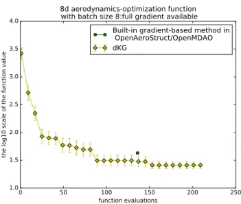
We evaluate thedKGalgorithm on the eight-dimensional aerostructural optimization problem defined in the OpenMDAO test suite and available athttps://github.com/mdolab/OpenAeroStruct. This model couples a vortex-lattice method and a three-dimensional beam model to simulate aerostructural analysis of a wing. We compare the performance ofdKGto the default gradient-based optimization algorithm SLSQP provided by the OpenMDAO framework. dKGoutperforms SLSQP and additionally has the advantage that it provides good solutions already at low computational cost. Note thatdKG chooses eight designs in batch in each iteration and evaluates these designs simultaneously. In this benchmarks, all partial derivatives are available, thusdKGobserves 72 (=q(d+ 1)) values at each iteration. Fig. 2 shows the performances of dKGand the gradient-based optimizer SLSQP.
Figure 2: Combining Bayesian and gradient-based optimization,dKGoutperforms the gradient-based opti-mization algorithm of OpenMDAO on an aerostructural test problem. dKGselects batches of eight points to be evaluated in parallel.
The source code of thedKGalgorithm is available athttps://github.com/wujian16/Cornell-MOE.
V.
Conclusions
In this paper, we reviewed two BO algorithms adapted for the optimization of expensive-to-evaluate aerospace engineering systems. BO sequentially updates a statistical model that is used to select the next design to evaluate, reducing the number of calls to the expensive function. Each algorithm presented addresses a particular challenge encountered in aerospace engineering.
The first algorithm,rollout, selects the next design to evaluate in order to maximize the expected feasible improvement obtained over several steps. It allows for the optimization of systems subject to nonlinear expensive-to-evaluate inequality constraints, a common situation in aerospace engineering. Accounting for the long-term e↵ect of a decision was shown to improve the optimization performance. Such benefits were demonstrated on a reacting flow problem.
The second algorithm, dKG, leverages sensitivity information, such as gradients computed via adjoint methods, to improve the statistical model and select a batch of designs to evaluate at each iteration. This was shown to outperform a gradient-based optimization algorithm on an aerostructural optimization problem.
The two BO algorithms reviewed in this paper have been demonstrated to improve performance on several aerospace design problems. They are promising tools for the aerospace engineer and have the potential to further enable the global optimization of expensive-to-evaluate functions.
Acknowledgment
The methods described in this paper were developed for the fidelity, information source, Multi-physics (M3) project as part of the U.S. Air Force Office of Scientific Research (AFOSR) Multidisciplinary
Research Program of the University Research Initiative (MURI). The authors gratefully acknowledge the support of AFOSR Award Number FA9550-15-1-0038, program manager Dr. Jean-Luc Cambier.
References
1Jones, D. R., Schonlau, M., and Welch, W. J., “Efficient Global Optimization of Expensive Black-box Functions,”Journal
of Global Optimization, Vol. 13, No. 4, 1998, pp. 455–492.
2Brochu, E., Cora, V. M., and De Freitas, N., “A Tutorial on Bayesian Optimization of Expensive Cost Functions, with Application to Active User Modeling and Hierarchical Reinforcement Learning,”arXiv preprint arXiv:1012.2599, 2010.
3Lam, R. R. and Willcox, K. E., “Lookahead Bayesian Optimization with Inequality Constraints,”Advances in Neural
Information Processing Systems 30, 2017, pp. 1888–1898.
4Lam, R. R., Willcox, K. E., and Wolpert, D. H., “Bayesian Optimization with a Finite Budget: An Approximate Dynamic Programming Approach,”Advances in Neural Information Processing Systems, 2016, pp. 883–891.
5Wu, J., Poloczek, M., Wilson, A., and Frazier, P., “Bayesian Optimization with Gradients,”Advances in Neural Information
Processing Systems, 2017, Accepted for publication.
6Krige, D. G., “A Statistical Approach to Some Basic Mine Valuation Problems on the Witwatersrand,”Journal of the
Southern African Institute of Mining and Metallurgy, Vol. 52, No. 6, 1951, pp. 119–139.
7Matheron, G., “The Theory of Regionalized Variables and its Applications.”Les Cahiers de Morphologie Mathematique
(Fontainebleau). Fasc. 5. 218 p., 1971.
8Simpson, T. W., Mauery, T. M., Korte, J. J., and Mistree, F., “Kriging Models for Global Approximation in Simulation-based Multidisciplinary Design Optimization,”AIAA Journal, Vol. 39, No. 12, 2001, pp. 2233–2241.
9Rasmussen, C. E. and Williams, C. K. I.,Gaussian Processes for Machine Learning, MIT Press, Cambridge, MA, 2006. 10Lizotte, D. J.,Practical Bayesian Optimization, Ph.D. thesis, University of Alberta, 2008.
11Srinivas, N., Krause, A., Kakade, S. M., and Seeger, M., “Gaussian Process Optimization in the Bandit Setting: No Regret and Experimental Design,”Proceedings of the 27th International Conference on Machine Learning, 2010, pp. 1015–1022.
12Queipo, N. V., Haftka, R. T., Shyy, W., Goel, T., Vaidyanathan, R., and Tucker, P. K., “Surrogate-based Analysis and Optimization,”Progress in Aerospace Sciences, Vol. 41, No. 1, 2005, pp. 1–28.
13Wang, G. G. and Shan, S., “Review of Metamodeling Techniques in Support of Engineering Design Optimization,”Journal
of Mechanical Design, Vol. 129, No. 4, 2007, pp. 370–380.
14Forrester, A. I. J. and Keane, A. J., “Recent Advances in Surrogate-based Optimization,”Progress in Aerospace Sciences, Vol. 45, No. 1, 2009, pp. 50–79.
15Viana, F. A. C., Simpson, T. W., Balabanov, V., and Toropov, V., “Metamodeling in Multidisciplinary Design Optimization: How Far Have We Really Come?” AIAA Journal, Vol. 52, No. 4, 2014.
16Schonlau, M., Welch, W. J., and Jones, D. R., “Global Versus Local Search in Constrained Optimization of Computer Models,”Lecture Notes-Monograph Series, 1998, pp. 11–25.
17Sasena, M. J., Papalambros, P., and Goovaerts, P., “Exploration of Metamodeling Sampling Criteria for Constrained Global Optimization,”Engineering Optimization, Vol. 34, No. 3, 2002, pp. 263–278.
18Picheny, V., Gramacy, R. B., Wild, S., and Le Digabel, S., “Bayesian Optimization Under Mixed Constraints with a Slack-variable Augmented Lagrangian,”Advances in Neural Information Processing Systems, 2016, pp. 1435–1443.
19Audet, C., Denni, J., Moore, D., Booker, A., and Frank, P., “A Surrogate-model-based Method for Constrained Optimization,”8th Symposium on Multidisciplinary Analysis and Optimization, 2000.
20Sasena, M. J., Papalambros, P. Y., and Goovaerts, P., “The Use of Surrogate Modeling Algorithms to Exploit Disparities in Function Computation Time within Simulation-based Optimization,”Constraints, Vol. 2, 2001, pp. 5.
21Gramacy, R. B. and Lee, H. K. H., “Optimization Under Unknown Constraints,”arXiv preprint arXiv:1004.4027, 2010. 22Picheny, V., “A Stepwise Uncertainty Reduction Approach to Constrained Global Optimization.”AISTATS, 2014, pp. 787–795.
23Gardner, J., Kusner, M., Weinberger, K. Q., Cunningham, J., and Xu, Z., “Bayesian Optimization with Inequality Constraints,” Proceedings of the 31st International Conference on Machine Learning (ICML-14), JMLR Workshop and Conference Proceedings, 2014, pp. 937–945.
24Feliot, P., Bect, J., and Vazquez, E., “A Bayesian Approach to Constrained Single-and Multi-objective Optimization,”
Journal of Global Optimization, Vol. 67, No. 1-2, 2017, pp. 97–133.
25Bj¨orkman, M. and Holmstr¨om, K., “Global Optimization of Costly Nonconvex Functions Using Radial Basis Functions,”
Optimization and Engineering, Vol. 4, No. 1, 2000, pp. 373–397.
26Gramacy, R. B., Gray, G. A., Le Digabel, S., Lee, H. K. H., Ranjan, P., Wells, G., and Wild, S. M., “Modeling an Augmented Lagrangian for Blackbox Constrained Optimization,”Technometrics, Vol. 58, No. 1, 2016, pp. 1–11.
27Gelbart, M. A., Snoek, J., and Adams, R. P., “Bayesian Optimization with Unknown Constraints,”arXiv preprint
arXiv:1403.5607, 2014.
28Hern´andez-Lobato, J. M., Gelbart, M. A., Adams, R. P., Ho↵man, M. W., and Ghahramani, Z., “A General Framework for Constrained Bayesian Optimization using Information-based Search,”arXiv preprint arXiv:1511.09422, 2015.
29Hern´andez-Lobato, J. M., Gelbart, M. A., Ho↵man, M. W., Adams, R. P., and Ghahramani, Z., “Predictive Entropy Search for Bayesian Optimization with Unknown Constraints,”Proceedings of the 32nd International Conference on Machine Learning, Lille, France, 2015.
30Bu↵oni, M. and Willcox, K. E., “Projection-based Model Reduction for Reacting Flows,”40th Fluid Dynamics Conference
and Exhibit, 2010, p. 5008.
31Lions, J. L.,Optimal Control of Systems Governed by Partial Di↵erential Equations, Vol. 170, Springer Verlag, 1971. 32Jameson, A., “Aerodynamic Design via Control Theory,”Journal of Scientific Computing, Vol. 3, No. 3, 1988, pp. 233–260. 33Reuther, J. J., Jameson, A., Alonso, J. J., Rimlinger, M. J., and Saunders, D., “Constrained Multipoint Aerodynamic Shape Optimization using an Adjoint Formulation and Parallel Computers, Part 2,”Journal of Aircraft, Vol. 36, No. 1, 1999, pp. 61–74.
34Giles, M. B. and Pierce, N. A., “An Introduction to the Adjoint Approach to Design,”Flow, Turbulence and Combustion, Vol. 65, No. 3-4, 2000, pp. 393–415.
35Giles, M. B. and S¨uli, E., “Adjoint Methods for PDEs: A Posteriori Error Analysis and Postprocessing by Duality,”Acta
Numerica, Vol. 11, 2002, pp. 145–236.
36Martins, J. R. R. A., Alonso, J. J., and Reuther, J. J., “A Coupled-adjoint Sensitivity Analysis Method for High-fidelity Aero-structural Design,”Optimization and Engineering, Vol. 6, No. 1, 2005, pp. 33–62.
37Biros, G. and Ghattas, O., “Parallel Lagrange–Newton–Krylov–Schur Methods for PDE-Constrained Optimization. Part I: The Krylov–Schur Solver,”SIAM Journal on Scientific Computing, Vol. 27, No. 2, 2005, pp. 687–713.
38Plessix, R.-´E., “A Review of the Adjoint-state Method for Computing the Gradient of a Functional with Geophysical Applications,”Geophysical Journal International, Vol. 167, No. 2, 2006, pp. 495–503.
39Adler, R. J., “The Geometry of Random Fields,”Wiley, London, 1981. 40Papoulis, A., “Random Variables, and Stochastic Processes,” 1990.
41Morris, M. D., Mitchell, T. J., and Ylvisaker, D., “Bayesian Design and Analysis of Computer Experiments: Use of Derivatives in Surface Prediction,”Technometrics, Vol. 35, No. 3, 1993, pp. 243–255.
42Yamazaki, W., Rumpfkeil, M. P., and Mavriplis, D. J., “Design Optimization Utilizing Gradient/Hessian Enhanced Surrogate Model,”28th AIAA Applied Aerodynamics Conference, Vol. 4363, 2010, p. 2010.
43Han, Z.-H., G¨ortz, S., and Zimmermann, R., “Improving Variable-fidelity Surrogate Modeling via Gradient-enhanced Kriging and a Generalized Hybrid Bridge Function,”Aerospace Science and Technology, Vol. 25, No. 1, 2013, pp. 177 – 189.
44Chung, H. and Alonso, J. J., “Using Gradients to Construct Cokriging Approximation Models for High-dimensional Design Optimization Problems,”40th AIAA Aerospace Sciences Meeting & Exhibit, Vol. 317, 2002, pp. 14–17.
45Lukaczyk, T., Palacios, F., Alonso, J. J., and Constantine, P. G., “Active Subspaces for Shape Optimization,”Proceedings
of the 10th AIAA Multidisciplinary Design Optimization Conference, 2014, pp. 1–18.
46Osborne, M. A., Garnett, R., and Roberts, S. J., “Gaussian Processes for Global Optimization,” 3rd International
Conference on Learning and Intelligent Optimization (LION3), Citeseer, 2009, pp. 1–15.
47Koistinen, O.-P., Maras, E., Vehtari, A., and J´onsson, H., “Minimum Energy Path Calculations with Gaussian Process Regression,”Nanosystems: Physics, Chemistry, Mathematics, Vol. 7, No. 6, 2016.
48Ahmed, M. O., Shahriari, B., and Schmidt, M., “Do We Need “Harmless” Bayesian Optimization and “First-Order” Bayesian Optimization?” NIPS BayesOpt, 2016.
49Scott, W., Frazier, P. I., and Powell, W., “The Correlated Knowledge Gradient for Simulation Optimization of Continuous Parameters Using Gaussian Process Regression,”SIAM Journal on Optimization, Vol. 21, No. 3, 2011, pp. 996–1026.