Spatial and temporal trends of phytoplankton and physiochemical variables in a hypertrophic, monomictic lake

(1)

http://researchcommons.waikato.ac.nz/

Research Commons at the University of Waikato

Copyright Statement:

The digital copy of this thesis is protected by the Copyright Act 1994 (New Zealand). The thesis may be consulted by you, provided you comply with the provisions of the Act and the following conditions of use:

 Any use you make of these documents or images must be for research or private study purposes only, and you may not make them available to any other person.  Authors control the copyright of their thesis. You will recognise the author’s right

to be identified as the author of the thesis, and due acknowledgement will be made to the author where appropriate.

 You will obtain the author’s permission before publishing any material from the thesis.

(2)

of phytoplankton and physiochemical variables

in a hypertrophic, monomictic lake

A thesis

submitted in partial fulfilment

of the requirements for the degree

of

Master of Science in Biological Sciences

at

The University of Waikato

by

BERNARD MICHAEL SIMMONDS

________________________________ The University of Waikato

(3)

(4)

Abstract

Spatial and temporal variations in the physical, chemical and biological composition of Lake Ōkaro were measured over 16 months. Lake Ōkaro is a small (0.32 km2) hypertrophic, monomictic lake located in the Central Volcanic Zone of the North Island, New Zealand. Vertical profiles of temperature, chlorophyll fluorescence, dissolved oxygen concentration (DO), pH, specific conductance, photosynthetically active radiation (PAR) and nutrient species, including ammonium-nitrogen (NH4-N), nitrite-nitrogen (NO2-N), nitrate-nitrogen (NO3-N) and phosphate-phosphorus (PO4-P), were collected at up to nine stations at weekly to monthly frequencies. High-frequency variability was assessed during two separate 24-hour monitoring periods, coinciding with an Anabaena spiroides -dominated surface bloom, and a Ceratium hirundinella-dominated deep chlorophyll maximum. Additional data for wind direction and velocity, incident solar irradiance and rainfall was sourced from a meteorological weather station and a lake monitoring buoy at Rotorua, 20 km north of the lake.

Spatial variability was more pronounced during summer. Observed vertical gradients in chlorophyll fluorescence, DO, specific conductance and nutrient species were closely linked to thermal stability of the water column. There were large variations in chlorophyll fluorescence amongst stations in summer, which related to displacement of the metalimnion and associated changes in chlorophyll fluorescence. Winter mixing was characterised by relative homogeneity of the water column. Nutrient concentrations were elevated at all depths whereas high concentrations had previously been confined to lower depth strata (the hypolimnion).

(5)

Temperature profiles in summer displayed clear vertical gradients with a well-defined metalimnion that increased in depth until winter mixing generated isothermal conditions. Chlorophyll fluorescence profiles were characterised by the formation of a DCM that was recurrent over both summer periods, and was strongly statistically related to the depth of the thermocline for the duration of stratification. Dissolved oxygen, specific conductance and pH were relatively uniform horizontally, though pH was consistently lower at a well-sheltered near-shore station. All variables showed strong variations with depth during the stratified period. Dissolved oxygen was negligible or zero below the thermocline for much of the stratified period while specific conductance was lowest above or at the thermocline. There were also strong vertical gradients in nutrient concentrations in summer, with concentrations below the thermocline often an order of magnitude higher than those above.

The representativeness of fluorescence at a central station to a whole-lake scale was assessed using a vertical integrated value and the standard error derived from up to eight other stations. Values at the single station frequently deviated from the mean fluorescence of the wider lake, particularly at the DCM which suggests that extrapolating single-station measurements to a whole lake could provide highly exaggerated values of lake fluorescence.

High-frequency sampling during the A. spiroides-dominated surface bloom showed diel temperature variations attributed mostly to solar irradiance. There was high light attenuation from the high phytoplankton biomass and consistently elevated pH and DO. Fluorescence profiles suggested that the phytoplankton population was strongly buoyant and did not undergo diel vertical migration.

(6)

High-frequency sampling during a period when there was a dinoflagellate-dominated DCM showed two coinciding fluorescence peaks had formed at 6-7 and 7-8 m depth and contained morphologically and physiologically distinct taxa. The 6-7 m DCM was predominantly Ceratium hirundinella, while the 7-8 m DCM was composed of C. hirundinella and unidentified colonial picoplankton. Fluorescence profiles suggested diel vertical migration was not taking place, and strong gradients in light, nutrient availability and the relative biomass of the dominants suggested that the 6-7 and 7-8 m DCM populations potentially differed in their modes of nutrition, light history and susceptibility to grazing.

This research illustrates the degree of spatial variability that can exist in a small, monomictic hypertrophic lake at a given time, and highlights some of the potential limitations of using single-site monitoring stations to represent the physical, chemical and biological conditions of a whole lake. This information may be used to critically evaluate the reliability of phytoplankton biomass estimates that have been derived from spatially-limited sampling methods. This study further illustrates the role that thermal stratification plays in creating vertical gradients in a number of biological and chemical variables, and demonstrates that parallels exist with regard to DCM formation in oligotrophic and hypertrophic lakes, relating to the interplay between light, chlorophyll fluorescence and thermal stratification. Evidence is also provided showing that diel-scale variations in phytoplankton biomass can differ markedly between a cyanobacteria-dominated surface bloom and a dinoflagellate-dominated DCM, which further highlights the value of high-frequency sampling when seeking to estimate phytoplankton biomass using in situ methods.

(7)

Acknowledgements

First and foremost I would like to thank my supervisor Professor David Hamilton for taking me on as a M.Sc. student back when I had little more than some summer experience in phytoplankton counting. Your enthusiasm has been a great source of motivation and you have always found ways of making things challenging and interesting, ensuring I have learned an immense amount along the way. I thank you for fostering my interests in limnology, and for helping to build the platform that will launch me toward a great future in science.

I would like extend my gratitude to Dr Deniz Özkundakci for his support over the past year. Your seemingly endless knowledge of Lake Ōkaro has been a fantastic source of information, and you have always been ready to lend an ear, offer advice and drink a coffee. Thanks for everything.

Thank you to Dr Susie Wood (Cawthron) for being there from my very first day as David‘s M.Sc. student. You have always been so encouraging, and I truly appreciate all the advice and feedback you have provided along the way.

A very special thanks to my field buddy Marie Dennis for two years of boat trips (rain or shine), early starts and late finishes, the countless coffee stops and all the hard work you‘ve put in collecting and processing my samples. I‘ve been tremendously lucky to be able to count on you.

I would like to acknowledge Wendy Paul for helping to identify phytoplankton, teaching me lab methods, providing equipment, proof reading drafts and always being there to lend an ear and have a chat. Thank you for all your help over the past two years.

(8)

I would also like to express thanks to Kohji Muraoka. You have always been ready to drop everything and offer advice, or just get out of the office for Goura and coffee. Sharing a flat over the past year has been a blast, and I‘m blessed to call you a friend.

All my love to my dad Mike, my mum Sue, and my brothers Tim, Andrew and Nick. Thanks for being there over the past few years; particularly when things have gotten tough and I‘ve needed to escape for some awesome home cooked food and relaxation. You guys are the best.

Thanks to my partner Alyse Dombroski, for leaving your key out on cold winter nights when I‘ve had to work late, for bringing me cooked meals and for all your support during those stressful times.

I would like to acknowledge the hard work of Louise Stewart for running my nutrient samples and for teaching me how to do chlorophyll a analysis. Thanks to Sean Taylor of Scion, for the calibration and occasional operation of the flow cytometer. Thanks to Andreas Rueckert and Sarah Kelly for helping me with ARISA and for allowing me to culture cyanobacteria. Thank you to Barry O‘Brien for teaching me the ways of the IX-71 microscope, and for your perseverance in identifying the ―mystery Lake Ōkaro chlorophyte‖.

A special thanks to my good friend Brennan Mahoney and to the M.Sc. students, doctoral candidates and staff of the biology department for all the coffees and hilarious conversations. I wish you all the best for the future.

Finally, I am grateful for the financial support provided by the University of Waikato in the form of a research scholarship that has kept me fed with a roof over my head for the past two years.

(9)

List of figures

Figure 2.1: Map of Lake Ōkaro showing sampling stations and location of the

inflows and outflow (modified from Özkundakci et al. (2010)). 23

Figure 3.1: Thermocline depth and peak fluorescence depth of a shallow station

(S2) and a deep station (W1) from 01 December 2009 – 11 March 2011, and euphotic depth at station S1 from 17 December 2009 – 29 March 2011. 35

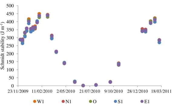
Figure 3.2: Schmidt stability at deep stations (station names are given on the inset)

from 01 December 2009 – 11 March 2011. 37

Figure 3.3: Depth of peak fluorescence with mean thermocline depth at deep

stations (station names are given on the inset) from 01 December 2009 – 11 March 2011. No thermocline was present from 01 June 2010 until 28 September

2010. 38

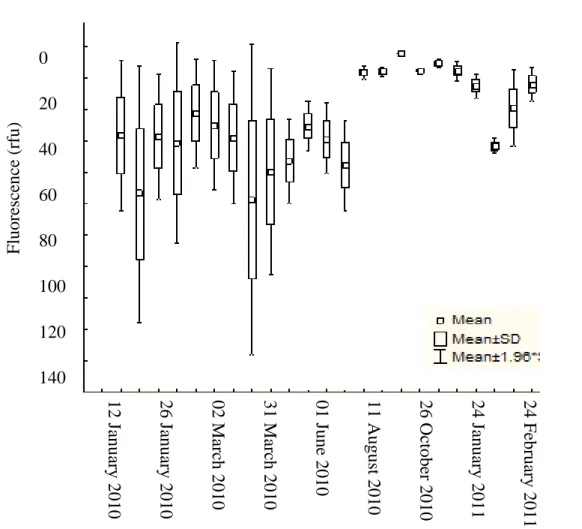
Figure 3.4: Mean values of chlorophyll fluorescence at deep stations (W1, N1, O,

S1 and E1) from 01 December 2009 to 11 March 2011. 39

Figures 3.5a-f: Temperature profiles for all stations from 01 December 2009 – 05

January 2010. 41

Figures 3.5g-o: Temperature profiles for all stations from 12 January 2010 – 01

June 2010. 42

Figures 3.5p-x: Temperature profiles for all stations from 29 June 2010 – 11

(14)

Figures 3.6a-i: Fluorescence profiles for all stations from 01 December 2009 – 26

January 2010. 45

Figures 3.6j-r: Fluorescence profiles for all stations from 02 February 2010 – 28

September 2010. 46

Figures 3.6s-v: Fluorescence profiles for all stations from 26 October 2010 – 10

February 2011. 47

Figures 3.7a-c: Dissolved oxygen profiles for all stations from 12 December

2009 to 22 December 2009. 48

Figures 3.7d-l: Dissolved oxygen profiles for all stations from 29 December 2009

to 31 March 2010. 49

Figures 3.7m-u: Dissolved oxygen profiles for all stations from 27 April 2010 to

11 February 2011. 50

Figures 3.7v-w: Dissolved oxygen profiles for all stations from 24 February 2011

to 11 March 2011. 51

Figures 3.8a-i: pH at all stations from 01 December 2009 to 26 January 2010.

52

Figures 3.8j-r: pH at all stations from 02 February 2010 to 28 September 2010.

53

Figures 3.8s-u: pH at all stations from 26 October 2010 to 24 January 2011.

54

Figures 3.9a-i: Specific conductance for all stations from 01 December 2009 to

(15)

Figures 3.9j-r: Specific conductance for all stations from 02 February 2010 to 28

September 2010. 56

Figures 3.9s-u: Specific conductance for all stations from 26 October 2010 to 24

January 2011 57

Figure 3.10a: Concentrations of NH4-N at 0, 3, 6, 9, 12 and 14 m depth in

samples taken from 01 December 2009 - 11 March 2011, and thermocline depth. Reference values are provided next to several sample points (mg L-1). 59

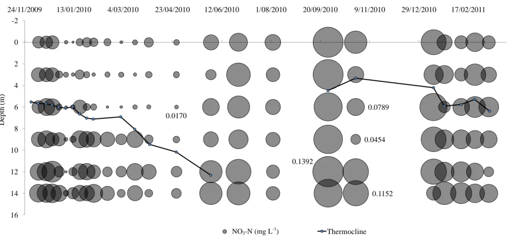
Figure 3.10b: Concentrations of NO3-N at 0, 3, 6, 9, 12 and 14 m depth in

samples taken from 08 December 2009 - 11 March 2011, and thermocline depth. Reference values are given next to several sample points (mg L-1). 60

Figure 3.10c: Concentrations of PO4-P at 0, 3, 6, 9, 12 and 14 m depth in

samples taken from 08 December 2009 - 11 March 2011, and thermocline depth. Reference values are given next to several sample points (mg L-1). 61

Figures 3.11a-i: Fluorescence (RFU) at central station and whole lake mean

fluorescence with standard error from 01 December 2009 to 26 December 2009. 63

Figures 3.11j-r: Fluorescence (RFU) at central station and whole lake mean

fluorescence with standard error from 02 February 2010 to 28 September 2010. 64

Figures 3.11s-u: Fluorescence (RFU) at central station and whole lake mean

fluorescence with standard error from 26 October 2010 to 10 February 2011. 65

(16)

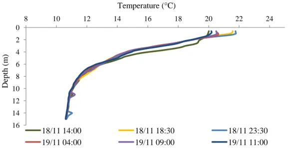
Figure 4.1: Temperature profiles for the sampling period of 19-20 November

2010. 67

Figure 4.2: Depth of the upper and lower metalimnion and of the thermocline on

18-19 November 2010. 67

Figure 4.3: Dissolved oxygen concentrations on 18-19 November 2010. 68

Figure 4.4: Specific conductance on 18-19 November 2010. 69

Figure 4.5: pH profiles on 18-19 November 2010. 70

Figure 4.6: Fluorescence on 18-19 November 2010. 71

Figure 4.7: Temperature profiles on 24-25 March 2011. 74

Figure 4.8: Depth of the upper and lower metalimnion, the thermocline and

Schmidt stability on 24-25 March 2011. 74

Figure 4.9: Dissolved oxygen concentrations on 24-25 March 2011. 75

Figure 4.10: Chlorophyll fluorescence and mean temperature profile on 24-25

March 2011. 76

Figure 4.11: Chlorophyll fluorescence in relative units, total cell concentrations

and phytoplankton biovolumes at 19:00 h on 25 March 2011. 78

Figure 9.1: Euphotic depth, Secchi depth and predicted euphotic depth (e.g.,

(17)

Figure 9.2: Image of Anabaena spiroides in Lake Ōkaro on 18-19 November 2010. Sample collected from 0 m depth at 11:00 h on 19 November 2010. Sample

concentration was 137,777 cells mL-1. 149

Figure 9.3a: 400x magnification of an unconfirmed species of chlorophyte

(picoplankton #2) collected from Lake Ōkaro on 23 March 2011 at 10 m depth.

Image courtesy of Barry O‘Brien. 149

Figure 9.3b: Picoplankton #2 at 1000x magnification, collected from Lake Ōkaro

on 23 March 2011 at 10 m depth. Image courtesy of Barry O‘Brien. 150

Figure 9.3c: Scanning electron microscope image of picoplankton #2 on tissue

paper (background), collected from Lake Ōkaro on 23 March 2011 at 10 m depth.

(18)

List of tables

Table 1.1 Limnological and catchment data for the 12 Te Arawa Lakes. Adapted

from Hamilton (2003) and Bay of Plenty Regional Council (2010). 14

Table 2.1: Limnological characteristics of Lake Ōkaro (adapted from Cronin et al.

(2006). 24

Table 2.2: Geographical position and depth of sampling stations with associated

sample methods. 25

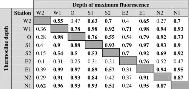
Table 3.1: Pearson correlation coefficient values for thermocline depth and depth

of maximum fluorescence for different stations (see Figure 2.1 for location of stations). Significant correlations (Ρ < 0.05) are shown in bold. 36

Table 4.1: Mean wind speed and direction at 3 hour intervals ON 18-19

November 2010. 72

Table 4.2: Light attenuation coefficients and euphotic depths for 25 March 2011.

75

Table 4.3: Peak and mean relative units and depths of DCM fluorescence (24-25

March 2011). 77

Table 4.4: Cell concentrations for sampled depths at 19:00, station W1, Lake

Ōkaro on the 25 March, 2011. 79

Table 4.5: Species biovolumes for sampled depths at 19:00, station W1, Lake

Ōkaro on the 25 March, 2011. Data are cells/mL-1 x biovolume (µm3). Biovolumes from Dryden & Vincent (1986) and Olenina et al. (2004). 80

(19)

Table 9.1: Light extinction coefficient (Kd, m-1), surface irradiance (I (0)), euphotic depth (zeu) and zeu irradiance (I(zeu)) from 17 December 2009 to 29

March 2011. 147

Table 9.2: Mean global irradiance between 06:00 h and 19:00 h from 16-19

November 2010. 148

Table 9.3: Wind data from 18-19 November 2010. Closest sample times are in

(20)

1

Introduction

1.1 Eutrophication

Eutrophication is defined as the nutrient enrichment of aquatic ecosystems, which frequently results in an array of symptomatic changes that impair water use (Likens et al., 1971). Where this process is exacerbated by anthropogenic activities it commonly known as ―cultural eutrophication‖ (Smith et al., 1999).

Many lakes are naturally eutrophic, particularly in warmer, temperate regions (Gannon and Stemberger, 1978). However, human population growth and changes in land use have accelerated rates of nutrient enrichment (Holling and Meffe, 1996, Hasler, 1969, Ehrlich and Holdren, 1971, Falkenmark, 1986), and cultural eutrophication has now been identified as the single most important form of detriment to global surface water quality (Smith and Schindler, 2009). The causal agents of cultural eutrophication are primarily activities that increase the bioavailability of naturally limiting elements for plant growth; nitrogen (N) and phosphorus (P) in water bodies. These include influxes of phosphorus containing detergents and cleaning products (Khan and Ansari, 2005), sewage and wastewater discharge (Smith, 2003), increased sedimentation from soil disturbances (Pimentel and Kounang, 1998) and agricultural land use practices with intensified stocking rates, and nitrogenous fertiliser applications (Glibert et al., 2006, Hamilton, 2005).

1.2 Eutrophication in New Zealand

Cultural eutrophication has become a major issue in New Zealand over the last century. Intensification of land use began in the 1920s with the development of

(21)

fertilisers and improvements in soil, animal and plant science (Molloy, 1980). By the 1970s, stocking rates had increased by 150% and the proportion of land converted for agriculture and exotic plantations had grown from 35% to 60% (Blaschke et al., 1992, MacLeod and Moller, 2006). Today, stocking rates and fertiliser usages have further increased (MacLeod and Moller, 2006), and high and low-producing grassland constitute 22% and 29% of the total land area, while exotic forestry covers a further 5% (MFE, 2010). Urbanisation, a known causal agent of eutrophication has increased rapidly. Urban centres currently comprise 0.6% of the total land area and contain 85% of the total population (Suren, 2000, Ministry for the Environment 2004). Declining water quality in NZ lakes is overwhelmingly consequential of cultural eutrophication, relating to total nitrogen (TN) and total phosphorus (TP) loading in areas of high intensity pastoral, exotic forestry, and urban land use (Abell et al., 2010).

1.3 Point source pollution

Waterways have long been used as convenient discharge sites for pollutants and organic wastes (Meybeck, 2003). Many of New Zealand‘s most significant lakes have a history of point source pollution. Direct inputs of phosphorus-treated sewage entered Lake Rotorua between 1973 and 1990 (Rutherford, 2003). In 1984-85, sewage-derived nutrients comprised 50% and 25% of the total load of TN and TP respectively, and in response to high TLI values and growing public concern for water quality, the regional council opted for land-based sewage disposal in the Whakarewarewa Forest from 1991 (Rutherford, 2003).

Lake Taupo is a 623 km2 oligotrophic lake on the central plateau of the North Island (Hawes and Smith, 1993). The majority of sewage is disposed of in septic tanks, and is treated within the lake catchment. In 1986, a small sewage treatment

(22)

plant was built less than 300 m from the lake shore (Hawes and Smith, 1993). Within three years, significant increases in nitrate-N concentrations were recorded as groundwater seepage contaminated a nearby tributary (Hawes and Smith, 1993).

1.4 Diffuse source pollution

The Resource Management Act (1991) effectively restricts activities that directly degrade fresh water resources, including many point source pollutants. However, diffuse inputs associated with the harvesting of exotic forestry and high-intensity pasture are known to be the dominant causal agents of external nutrient loading in many New Zealand lakes (Abell et al., 2011). In a study of 101 catchments throughout New Zealand, Abell et al. (2011) found exotic forestry represented 15.1% of the mean proportion of catchment type, and proportionally accounted for 18.8% of the variability in in-lake TP. In the same study, high-producing grassland was found to represent 33.1% of the mean catchment land use, and accounted for 38.6% and 41.0% of the variation in in-lake TN and TP respectively.

1.5 Consequences

The process of eutrophication often occurs in sequential steps. Nutrient enrichment is followed by increased primary productivity and succession in phytoplankton communities and typically culminates with the dominance of cyanobacterial species (Carpenter et al., 1998, Khan and Ansari, 2005). Long periods of phytoplankton growth exhaust dissolved inorganic nutrient concentrations in the epilimnion, and senescence transports nutrients in organic form to the hypolimnion which stimulates enhanced microbial decomposition, leading to hypolimnetic anoxia, and the regeneration of ammonium (Borowiak et al., 2010, Meersche et al., 2004). Phosphorus in the water column becomes

(23)

aggregated into insoluble flocculent and particulate organic forms which settle out and continue to bind P at the sediment/water interface. Aggregates dissolve under anoxic conditions, allowing soluble reactive phosphorus (SRP) to diffuse into the hypolimnion further perpetuating eutrophic symptoms by creating a positive feedback loop (Johannessen and Dahl, 1996, Bennion et al., 1996, Kalff, 2002a). Other attributes of a eutrophic water body can include the loss of biodiversity by creating favourable conditions for competitive exotic species (Codd, 2000, Geurts et al., 2008), reductions in water transparency, and unsuitability of water for stock or human consumption (van den Brandt and Smit, 1998).

1.6 Management options

Efforts to mitigate the symptoms of eutrophication are frequently aimed at reducing the availability of specific macronutrients for primary production (e.g. nitrogen and phosphorus), as nutrient availability is a key variable regulating phytoplankton community composition and biomass (Tilman et al., 1982).

External source reductions: Wetlands and riparian margins can intercept high proportions of catchment-derived P and N from reaching waterways (Woltemade, 2000, Osborne and Kovacic, 1993). Osborne & Kovacic (1993) tested the relative abilities of grass and forested buffer strips to assimilate nitrate-N, and dissolved and total phosphorus. Forested buffers removed up to 90% of nitrate-N in shallow groundwater, and grass systems removed a higher proportion of dissolved and total phosphorus (Osborne and Kovacic, 1993). In 2006, a 2.3 ha artificial wetland was constructed around Lake Ōkaro, predicted to remove 40% to 50% of the total nitrogen intercepted from the catchment (Sorrell, 2010). The extent of riparian vegetation around the lake margin has been increasing from 2006, as part of an ongoing lake restoration strategy (Cronin et al., 2006).

(24)

Bottom sediments are considered a source, as well as a sink of nutrients (Berg et al., 2004). Under anoxic conditions, concentrations of internally released nutrients can exceed those derived from external sources (Özkundakci et al., 2011). Sediment treatment options involve the application of chemical flocculants that bind to dissolved nutrients, predominantly phosphorus, reducing the proportion available for algal growth (Berg et al., 2004).

Attempts to reduce the in-lake concentrations of phosphate have been made using an aluminium sulphate solution (alum; 47% Al2(SO4)3·14H2O). In 2003, alum was applied to the epilimnion (0–3 m) of Lake Ōkaro with a target concentration of 0.6 g Al m3; considered to be low in comparison to other studies (Özkundakci et al., 2010). The application had limited long-term effects on internal loading (Paul et al., 2008), but other trials of alum at higher concentrations, while necessitating the use of a pH buffer in some cases, have been successful for periods up to 15 years (Cooke et al., 1993), with the best results typically recorded in the first 2-3 years (Søndergaard et al., 2007).

Another sediment capping agent; aluminium-modified zeolite (Z2G1) was evaluated in trials on Lake Ōkaro in 2007 and 2009, carried out by the Bay of Plenty Regional Council. The material has a high specific surface area and was engineered to have an enhanced nutrient uptake capacity for phosphorus over natural zeolite compounds (Özkundakci et al., 2010). The agent worked in a similar way to calcite described in Berg et al. (2004); forming a diffusion barrier by binding phosphate released at the sediment/water interface (Özkundakci et al., 2010).

Other management methods aim to disrupt the physical processes that support internal phosphorus loading and microbial regeneration of ammonium in lakes.

(25)

Hypolimnetic anoxia can be reduced by hypolimnetic oxygenation; the injection of oxygen in to the hypolimnion to concentrations where internal loading is minimised (Antenucci et al., 2005), or destratification, a mechanical process whereby bubbles are released from near the bottom sediment, simulating upwelling that erodes the base of the thermocline and reduces vertical gradients in oxygen, temperature and other dissolved and suspended particles (Schladow and Fisher, 1995).

Field & Prepas (1997) evaluated the effects of hypolimnetic oxygenation on zooplankton and phytoplankton communities in Amisk Lake, a large eutrophic lake in Alberta. The authors reported reduced phytoplankton biomass in surface waters after hypolimnetic oxygenation. Lackey (1973) used two aerators to destratify a mesotrophic reservoir with a surface area of 0.19 km2. Results were circumstantial, with decreases in overall phytoplankton biomass, but no changes in the biomass of the cyanobacteria Anabaena flos-aquae. Antenucci et al. (2005) evaluated the success of a ‗bubble plume‘ type of aerator in a storage reservoir with a surface area of 19.2 km2. Post-installation, concentrations of chlorophyll a

downstream from the aerator declined, and changes in the phytoplankton community; particularly relating to increases in low-light adapted species occurred. Dominance of the cyanobacteria Cylindrospermopsis raciborskii was not affected by aeration, however, an overall decline in chlorophyll a

concentrations was evident. The results of both studies indicate destratification may not be suitable as a management option for all problematic genera, particularly those that are competitive under low-light and nutrient limited conditions.

(26)

Reducing planktivorous fish abundances can stimulate a positive population response in zooplankton, intensifying the effects of grazing on primary producers. A number of studies have reported success using biomanipulation to enhance top-down regulation on cyanobacteria. For example, in enclosure experiments by Sarnelle (2007), the zooplankton Daphnia pulicaria significantly reduced the biomass of Microcystis aeruginosa; a potentially toxic cyanobacteria. Hambright et al. (2007) excluded planktivorous fish from nitrogen-rich ponds, alleviating predation on zooplankton (daphniid), and contrasted the effects of N:P ratios and zooplankton grazing on the abundance of N-fixing cyanobacteria. The study found that grazing pressure had the potential to affect cyanobacterial biomass at similar magnitudes to P-limitation.

1.7 Indicators of lake health

There are a variety of monitoring tools that quantitatively assess a lakes water quality and health as a function of its biological and chemical components. Ecological indicators relate the overall health and functioning of an ecosystem to the presence, diversity and abundance of key biological components. These can be used as early warning signals or indicators of trends (Niemi and McDonald, 2004). In some cases, an organism is so closely dependent on a narrow subset of conditions, that its very presence will confirm the existence of those conditions (Caro and O'Doherty, 1999). Biological indicators can be derived using the Two-way Indicator Species Analysis (TWINSPAN), a hierarchical method proposed by Hill (1979) that characterises habitats based on the presence of species with known ecological preferences (Dufrene and Legendre, 1997).

The health of lake macrophytes can reflect water quality. Lake Submerged Plant Indicators (LakeSPI) was developed by the National Institute of Water and

(27)

Atmospheric Research (NIWA), and assesses the extent, diversity and condition of native macrophytes in relation to the impacts of exotic invasive plants (Neilson et al., 2007, Caffrey et al., 2006). LakeSPI has been used by the Waikato Regional Council to detect changes in lake water quality stemming from decreases in the depth extent of submerged plants, and signs of stress relating to numbers of unattached plants (Neilson et al., 2007).

Macroinvertebrates have a wide range of tolerances to changing environmental conditions, including nutrient concentrations and water clarity. Populations reflect lake water quality, with sediments in poorer quality lakes tending to be dominated by highly tolerant Chironomidae and Oligochaeta (Neilson et al., 2007, Gabriels et al., 2010). Macroinvertebrates are increasingly used as bioindicators outside of New Zealand, and have become incorporated into United States and European Union standards for water quality assessments (Neilson et al., 2007). Rotifer assemblages can reflect lake trophic state. The Rotifer Community Index (Duggan et al., 2001) is a quantitative bioindicator that uses rotifer community composition to express lake trophic state, and has been adopted by the Waikato and Auckland regional councils (Fowler and Duggan, 2008).

Increasing cyanobacterial biomass is a common symptom of eutrophication (Smith, 2003). Resolving trends in phytoplankton succession, primary productivity and changes in community composition and biomass can assist in the early detection of declining water quality (Goldman, 1988, Cottingham and Carpenter, 1998). Routine monitoring for cyanobacterial cell concentrations had originally been used to alert authorities to degrading water quality in the Te Arawa lakes of the Bay of Plenty region (Wilding, 2001). From 2008, biovolume

(28)

calculations have been opted for as a more representative assessment of public health risk (Wood et al., 2008).

A combination of mean values for chlorophyll a concentration (a surrogate for algal biomass), Secchi depth, and total phosphorus (TP) constitute the Trophic State Index (TSI) proposed by Carlson (1977); a numerical indicator of lake health used classify trophic status (e.g TSI 50 < 70 eutrophic). Burns et al. (1999) modified the TSI for use in New Zealand lakes, which differ from northern hemisphere temperate lakes in that N more frequently limits productivity (Abell et al., 2010). The Trophic Level Index (TLI) predominantly differs from TSI in the inclusion of total nitrogen (TN) as a variable and a narrower numerical categorisation range. TLI is widely used by regional councils in New Zealand to identify long-term trends in water quality and set management goals (Rutherford, 2003).

Percent annual change (PAC) is used in conjunction with TLI, reducing the confounding influence of seasonal fluctuations in data by identifying significant changes in the four measured variables (chlorophyll a, Secchi depth, TP and TN) in relation to each other (Burns et al., 2009). PAC is based on the premise that key variables in a lake that has become more or less eutrophic should reflect the same degree of change toward trophic state by having similar PAC values (Burns et al., 2009).

Hypolimnetic anoxia is a symptom of increased primary productivity, and relates strongly to eutrophication (Borowiak et al., 2010). Volumetric Hypolimnetic Oxygen Demand (VHOD) describes the depletion rate of dissolved oxygen in the hypolimnion, and is regarded to be a reliable indicator of changes in organic matter generation and trophic state within lakes (Hamilton, 2006).

(29)

1.8 The importance of representative sampling

Natural ecosystems and their interacting components are complex, nonlinear, and often poorly understood (Holling and Meffe, 1996). Predictable outcomes that are expected are rarely obtained, partly because absolute representations of ecosystems are considered to be impossible in a statistical sense (Irvine et al., 2004). A major constraint of monitoring is that data derived from spatially-limited sampling programmes that do not encompass natural variability will not be representative of the wider lake environment. Results are further confounded when sampling is performed over temporal scales that exceed rates of natural change within the system.

A monitoring type that frequently falls into this category is phytoplankton monitoring (Heaney, 1976). The Rotorua Lakes‘ cyanobacterial monitoring programme procedure involves vertical tube samples from 0-1 m collected at weekly time scales from popular bathing sites. For the purposes of public health warnings for specific bathing locations, sampling at a weekly intensity may be sufficient to indicate general conditions. However, sampling at this spatial scale and frequency will typically miss around 30% of the spatial variability in chlorophyll across the lake (Kallio et al., 2003, Peters, 2002) and potentially omit major fluctuations in biomass that occur over relatively short time scales (Reynolds, 1984). Therefore, adequate sampling frequencies and spatially-representative sampling scales are paramount for studying lake-wide characteristics, such as changes in biomass or community composition. A major objective of any comprehensive sampling programme will be to first identify the spatial and temporal scales of variation that are relevant to the study.

(30)

1.9 Scales of variability in lakes

Spatiotemporal variability in the physical, chemical and biotic components of lacustrine ecosystems is a richly studied subject (Powell and Richerson, 1985, Pinel-Alloul and Ghadouani, 2007, Simon, 1976, Ganf and Oliver, 1982, George and Heaney, 1978). One of the most important physical characteristics of a lake is whether it becomes thermally stratified (Gorham and Boyce, 1989). The stability of thermal stratification is predominantly a function of lake depth, and ultimately determines the susceptibility of the water column to mixing (Kalff, 2002a).

In lakes with moderate stability, long periods of stratification are superimposed by short term mixing events relating to wind stress. These events can operate over a broad range of scales, influencing the distribution of phytoplankton, particulate matter and nutrients, reducing euphotic depth, and eroding temperature and oxygen gradients (Kalff, 2002a). Typical trends of succession in temperate lakes relate to the seasonal availability of light, nutrients and physical variables, including metalimnion development. Intermediate-sized temperate lakes frequently undergo a predictable sequence of succession (Reynolds, 1997b). During winter, the phytoplankton community is poorly diverse, consisting of centric diatoms and flagellates such as cryptophytes (Moss, 1973a, Grover and Chrzanowski, 2006). With increasing warmth and irradiance in spring, blooms of chrysophytes, diatoms, cryptophytes or chlorophytes occur, which are eventually suppressed by herbivorous grazers in late spring (Grover and Chrzanowski, 2006). The onset of stratification in summer results in the spatial segregation of nutrients and light, leading to the dominance of bloom-forming, buoyancy-regulating filamentous and colonial cyanobacterial genera (Reynolds, 1983). Microcystis is a colonial cyanobacteria genus that will typically outcompete Anabaena, a

(31)

filamentous cyanobacteria genus, by proliferating at a rapid rate over short time scales, before stabilising for long periods (Vincent and Dryden, 1989). However

Anabaena and Aphanizomenon have the added ability to fix atmospheric nitrogen, giving these genera a competitive advantage under N-limiting conditions (Reynolds, 1997b). Mixing depth increases in late summer to autumn, and under these conditions pennate and centric (particularly chain-forming, e.g. Aulacoseira

spp.) diatoms, dinoflagellates and filamentous cyanobacterial species predominate until populations crash with the onset of winter (Grover and Chrzanowski, 2006). The sequence follows a general pathway of decreasing growth rates and increasing investment in resource gathering, as nutrients and other variables become spatially segregated under stratified conditions (Reynolds, 1997b).

Phytoplankton primary productivity is a function of seasonally and spatially variable parameters, including temperature, light and nutrient availability, mixing depth and phytoplankton biomass and community composition (von Westernhagen et al., 2010). In a year-long study determining phytoplankton productivity rates (mg C m-3 h-1) in a deep, warm monomictic lake, productivity was found to be seasonally variable, and range over horizontal and vertical spatial scales (von Westernhagen et al., 2010). At 0 m depth, productivity increased 10 to 11-fold at some sites between January and April, yet this was not reflected at 5 m depth, where increases were marginal between November to April (von Westernhagen et al., 2010).

1.10 The Te Arawa Lakes

The central Taupo Volcanic Zone (TVZ) in the North Island is a c. 300 km-long, and 60 km-wide region of intense Quaternary silicic volcanism that has produced over 30 caldera-forming ignimbrite eruptions from 1.6 Ma, and resulted in the

(32)

formation of a number of lakes (Houghton et al., 1995, Wilson et al., 1995). The region is home to 12 of the 15 Te Arawa lakes, categorised by trophic state and mixing regime as ―eutrophic monomictic‖, ―mesotrophic monomictic‖, ―oligotrophic monomictic‖, and ―meso- and oligotrophic polymictic‖ (Hamilton, 2003). Trophic states of the Te Arawa Lakes correlate strongly with catchment land use, with higher proportions of exotic forest and pastoral land being associated with the poorest lake water quality (Table 1.1) (Bay of Plenty Regional Council 2010).

The lakes play a central role in attracting domestic and international tourism to the region (Bruesewitz et al., 2011). In the year ending December 1999, Rotorua was a destination for 30.2% of all international visitors to New Zealand (Horn and Simmons, 2002) and 18% of the total employment in the district was dependent on tourism (Fairweather and Simmons, 2000). The water quality of many of the Te Arawa Lakes has measurably declined and this is attributed to land use changes, predominantly the development and intensification of agricultural activities in the surrounding catchments (Özkundakci et al., 2009, Hamilton, 2005).

The Bay of Plenty Regional Council is responsible for managing 12 of the Te Arawa lakes. It uses a variety of monitoring strategies to assess lake water quality, including TLI (Burns et al., 1999), PAC, LakeSPI (Caffrey et al., 2006), and VHOD (Hamilton, 2006). Anchored high frequency monitoring buoys are also located on Lake Rotorua, Lake Rotoiti, Lake Tarawera, and Lake Rotoehu, and transmit data wirelessly to an online database, providing information on water column temperature at 2 m intervals, and dissolved oxygen concentration, phytoplankton pigment concentration (chlorophyll a), wind speed and other variables at 15-minute intervals (Zhang, 2010).

(33)

Table 1.1 Limnological and catchment data for the 12 Te Arawa Lakes. Adapted from Hamilton (2003) and Bay of Plenty Regional Council (2010).

Lake

2010 Trophic status (3 yearly average TLI)

Lake volume (km3) Catchment area (km2) Catchment to lake volume ratio (km-1) Average depth (m) Maximum depth (m) Agricultural land use (%) Rotorua Eutrophic (4.7) 0.802 482.0 601 11 45 65 Tarawera Oligotrophic (2.9) 2.274 150.0 66 50 87.5 32 Rotoiti Mesotrophic (3.9) 1.042 578.0 555 31 93.5 62 Rotomā Oligotrophic (2.6) 0.429 33.9 79 37 83 51 Rotoehu Eutrophic (4.5) 0.061 42.3 693 8 13 64 Ōkataina Oligotrophic (2.8) 0.466 63.6 136 39 79 16 Ōkareka Mesotrophic (3.3) 0.064 17.5 275 20 34 45 Rotokakahi Mesotrophic (4.0) 0.077 17.5 227 17.5 32 77 Rotomahana Mesotrophic (4.0) 0.479 89.0 185 60 125 57 Rerewhakaaitu Mesotrophic (3.7) 0.037 40.6 1107 7 15 86 Tikitapu Mesotrophic (3.0) 0.026 6.0 227 18 27.5 16 Ōkaro Hypertrophic (5.3) 0.003 3.6 1084 12.5 18 96

(34)

1.11 Lake Ōkaro

Lake Ōkaro (Figure 2.1) is a small hypertrophic, monomictic lake in the central North Island that has become increasingly eutrophic from the mid-1950s, with regular cyanobacterial blooms since the mid-60s (Forsyth et al., 1988). The decline in lake health has been attributed to agricultural intensification in the 3.89 km2 catchment, and in recent years major restoration initiatives have focused on reducing internal and external nutrient loading in the lake (Paul et al., 2008, Scholes, 2010, Cronin et al., 2006, Özkundakci et al., 2010).

1.12 Previous studies

Lake Ōkaro‘s phytoplankton biota has been studied in varying detail over the past five decades (Wood et al., 2009). In 1987, Lake Ōkaro and Lake Rotongaio were the focus of an international cyanobacterial dominance forum (Vincent et al., 1987). Research addressed the aspects of the lake environment thought to fundamentally influence cyanobacterial abundance, including mixed layer processes (Imberger and Spigel, 1987), zooplankton grazing (Burns et al., 1987), and attributes of key cyanobacterial genera, including nutrient requirements (Lean et al., 1987), buoyancy properties (Walsby and McAllister, 1987) and photosynthetic productivity (Robarts and Howard-Williams, 1987).

Wood et al. (2009) resolved the historical cyanobacterial communities of Lake Ōkaro using germination experiments and automated rRNA intergenic spacer analysis (ARISA). The authors found evidence of cyanobacteria in sediment cores dated at 100 BP, which suggested there had been no major changes in the akinete-producing cyanobacteria community composition over the past 100 years, and

(35)

supported studies which describe trends of increasing cyanobacterial abundance in Lake Ōkaro since the 1950s (Dryden and Vincent, 1986, Flint, 1977).

A year-long analysis of dominant phytoplankton biovolumes and community succession was carried out by Dryden & Vincent (1986), who noted changes in the algal community had occurred since the early 1970s, relating this to increased eutrophication. In a later study, Vincent & Dryden (1989) further resolved phytoplankton succession in Lake Ōkaro, noting temperature was closely correlated to major shifts in community composition, and that large population sizes were typically reached after long periods of slow, persistent growth. The study also found that nitrogen-limited conditions did not necessarily influence the abundance of nitrogen-fixing species, as Anabaena were absent during periods of NO3-N and NH4-N depletion when PO4-P concentrations were not considered limiting (Vincent and Dryden, 1989).

Nutrient availability is one of the many variables regulating phytoplankton community composition and biomass (Tilman et al., 1982). A mesocosm survey measuring physiological and growth rate responses of phytoplankton to changing N and P ratios in Lake Ōkaro was conducted by Lean et al. (1987). The study recognised N as the primary nutrient limiting growth in the epilimnion, with chlorophyll a concentrations increasing by 250% in enclosures where N was added singly. Phosphorus appeared to have a complimentary effect on phytoplankton growth when N was not limiting, with an 800% increase in chlorophyll a in enclosures treated with both N and P. Even in extremely phosphate-deficient conditions (as indicated by physiological assays), P did not stimulate growth on its own, and chlorophyll a concentrations declined in enclosures where only P was added.

(36)

Imberger & Spigel (1987) studied microstructure stratification profiles for a single day in Lake Ōkaro on 26 February 1987. The study used eight sampling stations around the lake to resolve water column stability under prevailing wind conditions. During the study, a thermocline was located at c. 7 m, and ―light and variable‖ wind of undisclosed velocity was found to be sufficient to cause internal wave activity (Imberger and Spigel, 1987). Water clarity was high enough to allow light to penetrate several metres, and stratification in the upper epilimnion was negligible, increasing the influence of wind mixing and boundary layer turbulence (Imberger and Spigel, 1987).

1.13 Scales of temporal variability

Temperatures in Lake Ōkaro are highly variable over the course of a year. During summer, surface waters reach up to 23 °C, decreasing to around 10 °C at the bottom of the water column. During isothermy temperatures decrease to a minimum of 8 °C (Dryden and Vincent, 1986, Vincent and Dryden, 1989). The stability of the metalimnion (resistance to mixing) varies over much shorter temporal scales, being regulated by surface heat flux, lake bathymetry, water clarity (biological activity and suspended solids), and wind (Imberger and Spigel, 1987, Vant and Davies-Colley, 1986, Davies-Colley, 1987).

The availability of nutrients for primary productivity is strongly influenced by the resistance of the water column to vertical mixing (Spigel and Imberger, 1987). As a warm monomictic lake, Lake Ōkaro undergoes a single extensive stable stratification period for c. 8 months of the year (Özkundakci et al., 2010). Schmidt stability; a measure of water column stability, is generally at its highest from December through January (Paul, 2006). The hypolimnion becomes anoxic for the

(37)

majority of the thermal stratification period (Özkundakci et al., 2011), and leads to internal loading of c. 2,410 kg N year, and 380 kg P year (Burns et al., 2009).

Lake Ōkaro is fully mixed for c. 4 months (Özkundakci et al., 2010). The depth of the metalimnion varies throughout the season, with an average depth of approximately 6 m (Dryden and Vincent, 1986, Paul, 2006). From May, atmospheric heat loss reduces the density gradient between the oxic surface and anoxic bottom waters, resulting in the erosion of the metalimnion and eventual overturn of the lake (Kalff, 2002a, Paul, 2006). With lake overturn, ammonium and sediment-derived P are resuspended into the epilimnion, becoming available for algal growth (Spears et al., 2006).

The phytoplankton community in Lake Ōkaro progresses through a sequence of successional steps through the year. The steps of the dominant taxa have been detailed by (Dryden and Vincent, 1986) as bloom-forming Microcystis and

Anabaena cyanobacterial species from summer through to winter, overlapped by centric diatoms in autumn and winter, and followed by colonial chlorococcaleans in spring (Dryden and Vincent, 1986).

1.14 Spatial variability

Spatial heterogeneity, or ―patchiness,‖ generally describes variability at horizontal scales between about 10 m and 100 km, and at vertical scales between about 0.1 m and 50 m (Mackas et al., 1985). Phytoplankton patchiness is a known characteristic of phytoplankton in small thermally-stratified lakes (George and Heaney, 1978, Fasham, 1978), and can be caused by a number of factors. These include boundary-layer mixing associated with complex benthic topography (Imberger and Spigel, 1987), the physical characteristics of the resident

(38)

phytoplankton (e.g. buoyancy or depth-regulation) (George and Heaney, 1978), up- and downwelling at lake margins (George and Heaney, 1978), horizontal gradients in nutrient inputs (Fee, 1976), spatial variability in grazing effects (Therriault and Platt, 1978), wind forcing and water currents (e.g. Langmuir circulation cells) (Horne and Schneider, 1995), and internal waves (George and Heaney, 1978).

Phytoplankton surface blooms are generally formed by cyanobacterial and dinoflagellate species, and are a feature of productive lakes (Serizawa et al., 2010). It is understood that accumulation at the water surface is an adaptive strategy to maximise photosynthesis (Reynolds et al., 1981). Spatial variability during a surface bloom is pronounced on a vertical scale by high concentrations of phytoplankton at or near the surface during calm conditions (Reynolds and Walsby, 1975), and on a horizontal scale by uneven distribution of surface biomass, due to the influence of wind stress (Regel et al., 2004).

Deep chlorophyll maxima: In highly transparent lakes, phytoplankton biomass may become concentrated at intermediate depths, forming a deep chlorophyll maxima (DCM) (Hamilton et al., 2010). Gervais (1998) and Grigorszky et al. (2003) state the vertical positioning of cells can relate to the avoidance of damaging ultraviolet light levels (Modenutti et al., 2004), vertical gradients in mixotroph and zooplankton grazing intensity (Tittel et al., 2003, Longhurst, 1976), depth-differential sinking of phytoplankton (Padisák et al., 2003b), elevated nutrient concentrations at or below a thermocline (Gervais, 1998), in situ growth of autotrophic or mixotrophic algae (Padisák et al., 2003b) and behavioural aggregations of flagellates (Cullen, 1982, Grigorszky et al., 2003). DCMs are considered to be a feature of oligotrophic lakes (Serizawa et al., 2010), and are

(39)

able to be formed when the euphotic depth exceeds the maximum depth of the epilimnion (Hamilton et al., 2010). The occurrence of DCM in hypertrophic and hypertrophic lakes is not widely reported, however, some evidence exists for DCM formation in lakes with lower water quality. Klausmeier & Litchman (2001) hypothesised that a DCM formation could occur in eutrophic lakes at a depth where two components necessary for algal growth were equally limiting (e.g. a vertical separation of light and limiting nutrients). Gervais et al. (2003) state that a nutrient-deficient epilimnion, coupled with a metalimnetic oxygen gradient and nutrient-rich, anoxic hyplimnion will support sub-surface maxima of cyanobacteria or cryptophytes in mesotrophic lakes.

The physical, chemical and biological processes of a lake all combine to produce a complex system that is highly variable both in space and time; from broad-scale weather patterns down to micro-scale cellular processes. In order to be considered representative, monitoring must encompass spatial and temporal scales that are relevant to the natural variability of the subject and its setting. Spigel & Imberger (1987) discuss the importance of accounting for the rapid response of phytoplankton cells to changes in nutrients and light. They state that in order to explain short-term variations in algal properties, one must first resolve the small length and time scales relevant to phytoplankton (Spigel and Imberger, 1987).

1.15 Overview and Objectives

An analysis of spatial and temporal variability of phytoplankton community composition and biomass, and the physicochemical parameters governing these variables, forms the basis for this body of work. It is intended that the knowledge gained therein will assist in the interpretation of how key processes influence Lake Ōkaro‘s phytoplankton biota.

(40)

Objectives:

 To capture the extent of the vertical and horizontal spatial variability of phytoplankton biomass, nutrients, temperature and other parameters over a 15-month period in eutrophic, monomictic Lake Ōkaro, including two consecutive summers, and to determine the underlying processes.

 To ascertain the effectiveness of using a central lake station to estimate the vertical fluorescence characteristics of the whole lake.

 To capture two periods of contrasting phytoplankton distribution; an early-summer cyanobacterial, and late-early-summer dinoflagellate, and to contrast the vertical spatial and short-term temporal features of these periods.

(41)

2 Methods

2.1 Study stations

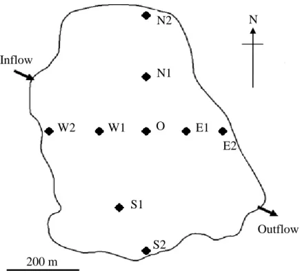
Lake Ōkaro (Figure 2.1) (38°17‘55.77‖S, 176°23‘41.09‖E) is a warm monomictic, caldera lake in the Waiotapu geothermal area of the central North Island, New Zealand (Hedenquist and Henley, 1985, Vincent et al., 1987). It is the most eutrophic of the 12 major Te Arawa Lakes. It has been the subject of a number of water quality studies and trials; several of which have focussed on restoration through reductions in internal or external nutrient loading (Özkundakci et al., 2010, Paul et al., 2008, Lean et al., 1987). The lake has a surface area of 0.32 km2, and average and maximum depths of 12 m and 18 m, respectively (Vincent et al., 1987). Lake Ōkaro‘s bathymetry has been described as ―complex‖ (Imberger and Spigel, 1987) because the bottom topography is characterised by several centrally-located low-lying ridges, the tallest of which rises 5 m from the benthos (Hardy, 2005). There are two main inflows from small unnamed streams that enter the north-west margin of the lake through a constructed wetland (Figure 2.1) (Özkundakci et al., 2011). The Haumi Stream is the only outflow, draining the lake at its southern end (Forsyth et al., 1988) (Figure 2.1). Water in the lake has a theoretical mean residence time of 1.5 years (Özkundakci et al., 2011). Over 95% of the lake catchment area of 3.67 km2 is exotic pasture and forest (Bay of Plenty Regional Council 2010) and agriculturally derived nutrients have supported recurrent blooms of cyanobacteria since the early 1960s (Hamilton, 2005, Forsyth et al., 1988, Özkundakci et al., 2010).

Lake Ōkaro is thermally stratified for around 8-9 months of the year. In the 2007-2008 period stratification persisted for 261 days, beginning intermittently as early as August and ending in mid-June (Özkundakci et al., 2011). From 1955 to 1964

(42)

Lake Ōkaro‘s hypolimnion became progressively anoxic as water quality declined (Forsyth et al., 1988). Bottom waters become deoxygenated within one month of thermal stratification (Gibbons-Davies, 2003), and remain anoxic (DO < 1 mg L-1) for the majority of stratification; typically persisting from late September to late May (Özkundakci et al., 2011). The extended periods of anoxia enhance internal nutrient loading, with estimates of 2410 kg N yr-1 and 380 kg P yr-1 from the bottom sediments (Burns et al., 2009). These high values mean major reductions in external loading are required in order to further improve the lake TLI. Lake water quality improved in the period 2007-2009 (Bay of Plenty Regional Council 2010), and the three-year average trophic level index (McFarland et al.) of 5.1 is consistent with a hypertrophic status (Scholes, 2010).

Figure 2.1: Map of Lake Ōkaro showing sampling stations and location of the inflows and

outflow (modified from Özkundakci et al. (2010)).

S2 Outflow Inflow s S1 E2 E1 O W1 W2 N1 N2 N 200 m

(43)

Table 2.1: Limnological characteristics of Lake Ōkaro (adapted from Cronin et al. (2006)

Lake Surface area 0.32 km2

Catchment area 367 ha (excluding lake) Lake surface height 423 m above sea level

Average depth 12 m

Deepest point 18 m

Trophic state Hypertrophic Annual mean TP (surface) 46.5 mg m-3 Annual mean TN (surface) 803.0 mg m-3

2.2 Field methods

Weekly monitoring was conducted from 1 December 2009 to 2February 2010, coinciding with thermally stratified conditions. Monthly monitoring began thereafter, concluding on 26 October 2010, and fortnightly monitoring resumed on 13 January 2011 and concluded on 11 March 2011. Routine monitoring included nine stations on Lake Ōkaro, including eight mid-lake and near-shore stations of north-south and east-west orientation, and one central lake station (Figure 2.1). Station S1 was at the deepest point in the lake (18 m), and is used by the Bay of Plenty Regional Council for routine monitoring as well as being used for earlier studies (Özkundakci et al., 2010, Vincent et al., 1987). Routine monitoring was performed between the hours of 08:00 h and 11:00 h, generally taking 1 h to complete. Station W1 was sampled over two separate 24-h periods (18 November, 2010 and 25 March, 2011) at intervals of 3-5 h.

(44)

Table 2.2: Geographical position and depth of sampling stations with associated sample methods

Station Coordinates Depth Samples taken (depths in brackets)

N1 38°17‘49.16‖S, _{176°23‘41.09‖E} 13.7 m

Seabird electronics probe (CTD) for temperature, conductivity, fluorescence, pH, dissolved oxygen, photosynthetically active radiation (PAR)

N2 38°17‘44.90‖S, 176°23‘41.09‖E 10.2 m CTD E1 38°17‘55.77‖S, 176°23‘45.87‖E 13.9 m CTD E2 38°17‘55.77‖S,

176°23‘51.77‖E 5.8 m CTD, dissolved nutrients (0, 3 m) O 38°17‘55.77‖S, _{176°23‘41.09‖E} 15.9 m CTD, dissolved nutrients (0, 3, 6, 9, 12, 14 m) S1 38°18‘02.32‖S, 176°23‘38.27‖E 18.0 m CTD, microscopy, chlorophyll a (0, 15 m) S2 38°18‘05.80‖S, 176°23‘41.09‖E 7.5 m CTD W1 38°17‘55.77‖S, 176°23‘36.29‖E 15.0 m CTD W2 38°17‘55.77‖S, _{176°23‘30.41‖E} 8.2 m CTD 2.3 Field measurements

A Seabird Electronics 19plus Seacat Profiler (Seabird Electronics, USA) hereby referred to as a CTD was used to resolve vertical profiles of temperature, pH, and conductivity, and was equipped with additional sensors for fluorescence (Turner Designs CYCLOPS-7), dissolved oxygen (SBE 43 Dissolved Oxygen Sensor), and photosynthetically active radiation (PAR) (LI-192SA Underwater Quantum Sensor). The CTD was deployed at all stations following a two-minute equilibration period. Profiles of fluorescence were checked for accuracy using biomass estimates derived from manual phytoplankton counts, with species biovolumes taken from taxonomic literature. On several occasions profiles were

(45)

also directly compared with chlorophyll a fluorescence from a second CTD (Chelsea Instruments Ltd) that was run at the same time.

A 10-L Schindler-Patellas trap was used to retrieve discrete depth samples. A breakdown of the subsample applications by station is given in Table 2. One sub-sample for microscopic enumeration was fixed immediately with 1% Lugols iodine solution, and stored in a 250 mL-1 specimen cup. Both preserved and unfixed samples were stored on ice in the dark. Additional phytoplankton samples were collected for microscopic enumeration from 0 m on 18 November, 2010, and from 0, 2, 4, 6, 7, 8, 9, and 10 m on 25 March, 2011 (station W1) and preserved with 1% Lugols solution.

Chlorophyll a samples were collected from depths of 0 m and 15 m (station S1). Samples were filtered immediately using a Swinnex 25 mm filter holder (Millipore), a Luer-Lok 60 mL-1 syringe (BD Biosciences) and a 0.45 µm glass fibre filter (GC50, Advantec). Filtered volume in each case was 60 mL-1. Filters were folded in half, immediately wrapped in aluminium foil and stored on ice in the dark.

The dissolved nutrient species ammonium (NH4-N), nitrite-nitrogen (NO2-N), nitrate-nitrogen (NO3-N), and dissolved reactive phosphorus (PO4-P) were collected from depths of 0 and 3 m (station E2), and 0, 3, 6, 9, 12, and 14 m (station O). Samples were filtered immediately with a Swinnex 25 mm filter holder (Millipore), a Luer-Lok 60 mL-1 syringe (BD Biosciences) 0.45 µm glass fibre filter (GC50, Advantec) and stored in 50 mL-1 polypropylene conical centrifuge tubes (Falcon, BD Biosciences), and kept in the dark, on ice, until transfer to the laboratory freezer (-20 °C) approximately 8 hours after collection.

(46)

2.4 High-frequency sampling

On 18 November 2010 and 25 March, 2011, station W1 was monitored at three-hourly frequency. The purpose of the monitoring was to examine sub-daily variations in the vertical distribution of phytoplankton chlorophyll and composition. At both stations CTD profiles were taken, and a laptop running Sea-Bird Seasave-Win32 and Sea-Sea-Bird DataProcessing-Win32 software (Seabird Electronics, USA) were used to resolve profiles of fluorescence immediately after each cast in order to then target points of interest for subsequent discrete depth sampling. Samples were collected using a Schindler-Patellas trap at 0 m (18 November, 2010), and 0, 2, 4, 6, 7, 8, 9, and 10 m (25 March, 2011), and fixed in 1% Lugols iodine.

2.5 Laboratory methods

Concentrations of nutrients NH4-N, NOx–N and PO4-P were determined using an AQUAKEM 200 cD discrete photometric analyser (Thermo Scientific). Standard AQUAKEM operating procedures were followed at all times. NO3-N was determined by subtracting NO2-N from NOx-N. NOx-N was analysed using Standard Methods using (SMWW/APHA Standard Method 4500 - NOx- E, and EPA Method 353.4 of Zhang et al. (1997) with a mean detection limit of 0.001 mg L-1). NO2-N concentrations were determined by SMWW/APHA Standard Method 4500 NO2- B with a mean detection limit of 0.001 mg L-1. PO4-P was analysed using Methods for the Examination of Water and Associated Materials: Phosphorus in Waters, Sewage and Effluents 1981. ISBN 011751582.5, and EPA Method 365.1 with a mean detection limit of 0.001 mg L-1. NH4-N was analysed for using Methods for the Examination of Water and Associated Materials: