Network Traffic Behavioral Analytics for Detection of DDoS Attacks

2019

Network Traffic Behavioral Analytics for Detection

of DDoS Attacks

Alma D. Lopez

Southern Methodist University, [email protected]

Asha P. Mohan

Southern Methodist University, [email protected]

Sukumaran Nair

Southern Methodist University, [email protected]

Follow this and additional works at:

https://scholar.smu.edu/datasciencereview

Part of the

Other Engineering Commons

This Article is brought to you for free and open access by SMU Scholar. It has been accepted for inclusion in SMU Data Science Review by an

Recommended Citation

Lopez, Alma D.; Mohan, Asha P.; and Nair, Sukumaran (2019) "Network Traffic Behavioral Analytics for Detection of DDoS Attacks,"

SMU Data Science Review: Vol. 2 : No. 1 , Article 14.

Network Traffic Behavioral Analytics for Detection of

DDoS Attacks

Alma Lopez1, Asha Mohan1and Sukumaran Nair2

1 _{Master of Science in Data Science, Southern Methodist University}

Dallas TX 75275, USA.

2

Director, AT&T Center for Virtualization, Southern Methodist University, Dallas TX 75275, USA.

{adlopez,asham}@smu.edu [email protected]

Abstract. As more organizations and businesses in different sectors are moving to a digital transformation, there is a steady increase in malware, facing data theft or service interruptions caused by cyberattacks on network or application that impact their customer experience. Bot and Distributed Denial of Service (DDoS) attacks consistently challenge every industry relying on the internet. In this pa-per, we focus on Machine Learning techniques to detect DDoS attack in network communication flows using continuous learning algorithm that learns the nor-mal pattern of network traffic, behavior of the network protocols and identify a compromised network flow. Detection of DDoS attack will help the network ad-ministrators to take immediate action and mitigate the impact of such attacks. DDoS attacks are costing enterprises anywhere between $50,000 to $2.3 mil-lion per year. We performed experiments with Intrusion Detection Evaluation Dataset (CICIDS2017) available from Canadian Institute for Cybersecurity to detect anomalies in network traffic. We use flow based traffic characteristics to analyze the difference in pattern between normal vs anomaly packet. We evaluate several supervised classification algorithms using metrics like maximum detec-tion accuracy, lowest false negatives predicdetec-tion, time taken to train and run. We prove that decision tree based Random Forest is the most promising algorithm whereas Dense Neural network performs equally well on certain DDoS types but require more samples to improve the accuracy of low sampled attacks.

1

Introduction

Distributed Denial of Service (DDoS) attacks pose a serious threat to all corporations that depend on network traffic and e-commerce. The DDoS attacks could bring down the operation and services of corporations leaving them with financial, reputational damage and customer dissatisfaction. DDoS attack can be performed against a network device or towards services provided by these devices and cause them heavy usage of CPU and memory that will preclude them from operating normally. With the dramatic growth of Internet of Things (IoT) and Bring Your Own Device (BYOD) principles, several new types of devices are accessing the network every day, exposing new vulnerabilities in

the network. The insecure devices can be compromised easily with the use of malware and ‘botnets’ that can launch Distributed DoS attack on the network.

Digital transformation is rapidly changing the architecture of data centers and more and more corporations are moving to Software Defined Networks (SDN). According to Radware Global Application and Network Security report 2016-173 and 2017-184, DDoS group’s typical tactics, techniques and procedure are to hack and infiltrate the victim’s data and demand a ransom payment in exchange for not publicly releasing the stolen data. There is a steady increase in the volume of the DDoS attacks from 2016 compared to 2018. In 2018 there was an increase in application-layer vs. network-layer attacks. The threats include IoT botnet-based DDoS attacks, DNS attacks, Advanced Persistent DDoS attacks, SSL/Encrypted attacks, Application layer attacks, Ransom DDoS attacks, Amplification attacks, Telephony DoS attacks and Content Delivery Net-work (CDN)-based attacks.

DoS attacks are accomplished by flooding the targeted machine with redundant re-quests that will overload and saturate the bandwidth and resources such that legitimate requests will get dropped. DDoS attacks are categorized in the way they are performed; broadly, the DDoS attacks can be classified as volume based attacks, protocol attacks and application layer attacks.

1.1 Type of DDoS attacks

Volume based attacks. These attacks often generate a huge volume of network traffic towards a target device and saturate the resources of the device under attack. Some of the common DDoS attacks are User Datagram Protocol (UDP) Flood, Internet Control message Protocol (ICMP) Flood, Synchronize (SYN) Flood etc.

Protocol based attacks. These attacks make use of the vulnerability present in specific protocol like Transmission Control Protocol (TCP) and Ping to consume the server resources thereby making their services unavailable to the legitimate users.

Application layer attacks. These attacks target a specific application layer proto-col like Hypertext Transfer Protoproto-col (HTTP) and generate protoproto-col packets in such a way that the server will have multiple long open sessions causing exhaustion of re-sources. The packets look very similar to a normal packet and is not detected by com-mon anomaly detection algorithms. Results in Q2 and Q3 2018 indicate SYN flood attack is the most common type of attack and contributes to 83.2% of DDoS attacks, UDP traffic is around 11.9% and HTTP is the third type of attack.

Slow and low rate attacks are much more difficult to detect as they are very close to a normal traffic. In this kind of attack, the attacker opens a session with the network device and keep it open for a long period of time, sending very low traffic. This way the network device will not idle timeout the attacker. The traffic appears legitimate to the traditional DDoS detection techniques and will not fall under the radar of common detection tools. When multiple sessions emerge very slowly and stay open for extended

3

https://mediaserver.responsesource.com/mediabank/18328/RadwareERTJan18/ RadwareERTReport20172018Finalreduced2.pdf

period of time, the slow and low attack will eventually exhaust the resources of the victim.

91% of security professionals in a survey done by Corero [2], a network security company, said that individual DDoS attacks can cost their organizations approximately $50,000 in lost business, attack mitigation, and lost productivity. Solution provider Kaspersky estimates between $1.2 - $2.3 million depending on the size of the busi-nesses under attack. Most impacting factor of a DDoS attack to online busibusi-nesses is the customer’s trust and confidence on the company.

Our goal is to build a generic statistical model after a comparative analysis of vari-ous machine learning algorithms that can be used to detect network anomaly. A network traffic flow analyzer can be used to capture flow information like duration, number of packets, number of bytes, lengths of the packets, etc. Later the network traffic features are built into a csv file consumed by machine learning models and evaluated speed and accuracy.

2

Related Work and Background

Several research papers are focused on intrusion detection and network traffic anomaly detection using various techniques. The research can be mainly divided into follow-ing technical categories; threshold or packet rate mechanisms to detect a flood based and protocol-based DDoS attacks, measuring uniformity of the packet for slow rate DDoS attacks. The rate limiting techniques are efficient in detecting the anomaly when the attacker launch connection to different victims in a short period of time. When the threshold is reached, the traffic is classified to have an anomalous behavior. Such re-search does not discuss in detail on how slow traffic based attack can be detected.

Some of the research focus mainly on the number of packets and ignore the time characteristics of DDoS attack or interval between the packets. M. Nugraha [3] uses openFlow to detect SYN flood attacks based on number of packets. Rodrigo Braga [4] propose using a lightweight method for DDoS attack detection using NOX/OpenFlow. Peng [5] proposal is to use simple source IP address Monitoring (SIM) to detect high bandwidth or flood-based attacks. The detection delay is high since the model monitors arrival rates of source IP addresses and detects changes in them. Some methods like Feinstein [6] use computing entropy and frequency-sorted distribution of specific IP attributes. Nevertheless, most of the existing research is based on CAIDA (Center for Applied Internet Data Analysis) dataset generated in 2007, or the DARPA 98 or KDD99 data sets that are available since 1998 and 1999 [7, 8]. Kokil [9] proposed SVM clas-sifier model with good accuracy but takes long time to train and generate detection model using DARPA dataset, also this paper does not take into consideration if detec-tion model on non-SDN dataset like DARPA can be extended to SDN network data packets. Zekri [10] proposed ML model based on flooding-based attack targeting layer 3 and layer 4 in the OSI 7-layer model in cloud architecture. Radford [11] researched on unsupervised anomaly detection, using natural language processing literature consider-ing the flow of packets as a ‘language’ between machines and used Recurrent Neural

Network for research on CICIDS2017. The accuracy of detection was less than 90% on most attacks.

In this paper we use CICIDS2017 dataset [12] that contains a mix of both benign traffic and the most up-to-date DoS attacks available publicly for research under Cana-dian Institute of Cybersecurity website. The data set includes the network traffic cap-tures parsed using CICFlowMeter [14] with labeled flows based on the time-stamp, source and destination IPs, source and destination ports, protocols and type of attack in a csv format file. In this paper, a subset of data from CICIDS2017 is taken to op-timize Machine Learning model that can be used to detect the following attacks: DoS slowloris, DoS slowhttptest, DoS generated using Hulk, Golden Eye, Botnets and LOIC generated DDoS.

Slowloris and Slowhttptest. These attacks are generated by keeping a single ma-chine’s connection open with minimal bandwidth that consumes the web server re-sources and take it down very fast.

Heartbleed. It is a security bug in the OpenSSL cryptography library and can scan vulnerabilities in the Transport Layer Security.

Hulk. This attack is designed to generate volumes of unique and obfuscated traffic at a webserver, bypassing caching engines and hitting the server’s direct resource pool.

GoldenEye. These attacks generate heavy load on HTTP servers in order to bring them down by exhausting resource pools. GoldenEye is a HTTP/S Layer 7 Denial-of-Service Testing Tool. It uses KeepAlive (and Connection: keep-alive) paired with Cache-Control options to persist socket connection busting through caching (when pos-sible) until it consumes all available sockets on the HTTP/S server.

Botnet.These attacks performed various tasks like spam through internet-interconnected devices to access the victim device.

DDoS. DDoS attacks were generated with Low Orbit Ion Canon (LOIC) which sent the UDP, TCP, or HTTP requests to the victim server.

3

Dataset

The dataset used in this research contains normal network flows and flows with DDoS attacks. The research team from Canadian Institute for Cybersecurity [12] generated the CICIDS2017 dataset. The team took as top priority to generate a realistic network traffic using a benign profile system (Sharafaldin, et al. 2016) [13] that abstracts behavior of human interactions and generates a naturalistic benign background traffic. DoS/DDoS attacks were captured on Wednesday July 5 and Friday July 7, 2017.

The data was created in a testbed infrastructure with two separated networks; Victim-Network and Attacker-Victim-Network. Research team included a victim-network router, fire-wall, switch and equipment with Windows, Linux and Macintosh operating systems. Attacker-network consists of router, one switch and four PCs.

3.1 Exploratory Data Analysis

Exploratory data analysis (EDA) was performed to understand the data captured in the traffic flow and features were generated by the network traffic analyzer CICFlowMeter [14]. Initial focus was on checking assumptions required for model fitting and hypothe-sis test, identifying missing values and performing variable transformations needed for the ML algorithms. The number of records available for Heartbleed attack was only 0.0016% of the dataset and so this attack was excluded from the analysis due to low number of samples.

There are 85 features provided by CICFlowMeter tool, appropriate features were extracted using Recursive Feature Elimination (RFE) techniques. Also feature impor-tance was checked as classification algorithms were run. The CICIDS2017 dataset is described in detail in research papers [13] for DoS/DDoS attacks. Selection of the ap-propriate features before a classification model can fit on the data is very important for the success of the model. Correlation between the features were analyzed to eliminate features that contribute the same information about the data.

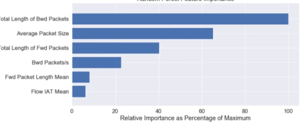
As part of identification of important features to detect anomaly, random forest fea-ture importance attribute was examined. This attribute shows how much the Gini Index for a feature decreases at each split. The more the Gini Index decreases for a feature, the more important the feature is. In this case, figure 1 shows features in the order of its importance: Total length of backward packets, average packet size, total length of forward packets, backward packets per second and flow duration are the key features.

In networks, flow is a session of packets between a source IP and port to a destina-tion IP and port. Forward flow is when the packet moves from say A to B and backward is when the reply for the packet moves from B to A.

Fig. 1.Feature importance for the Random Forest model.

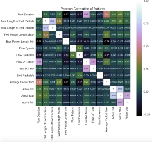
Correlation is a statistical method to analyze the relationship between a pair of vari-ables and indicates the multicollinearity in the data. For continuous varivari-ables, a corre-lation matrix with a Pearson’s correcorre-lation coefficient will define the linear recorre-lationship between two attributes. The correlation is in the range of -1 to +1 where +1 indicate that

there is a very strong positive relationship between the variables and -1 indicate that there is a very strong negative relationship between the variables. Figure 2 shows the correlation plot, the correlated features with a Pearson’s correlation coefficient greater than 0.8 were removed and more analysis was done using heatmap to check if there are redundant features in the data frame.

Fig. 2. Pearson’s correlation plot of the final features considered by statistical models in this paper.

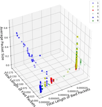
The group of attacks in the data set (anomaly different than 0) can be identified visually based on the three identified features: Average Packet Size, Total Length of Forward Packets and Total length of Backward Packets.

The scatter plot shown in figure 3 displays the attacks based on the three most important features identified.

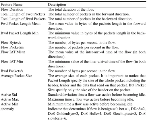
After the analysis, results for correlation and random forest importance feature we identified 14 features that were used in the final dataset used by the models in this paper, table 2 contains features details described by Sharafaldin paper [13].

Fig. 3.Scatter plot for the three most important features identified in Random Forest model for the flows with anomaly category with DoS/DDoS attack. Bot =1, DDoS=2, DoS GoldenEye=3, DoS Hulk=4, DoS Slowhttptest=5, DoS slowloris=6.

The total number of flows in the dataset is 1,109,470 which combines benign and DDoS attacked flows. Table 1 shows the distribution of number of flows for each DDoS types and benign packets. As seen in the table, benign packets contribute to 65% of the dataset and the remaining 35% belong to the anomaly. This also introduced class Imbalance problem in the models.

Table 1.Flows distribution.

Attack Anomaly indicator Number of flows

BENIGN- No Attack 0 726816 DoS Hulk 4 231073 DDoS 2 128027 DoS GoldenEye 3 10293 DoS slowloris 6 5796 DoS Slowhttptest 5 5499 Bot 1 1966

Table 2.Final Dataset Features Description.

Feature Name Description

Flow Duration The total duration of the flow.

Total Length of Fwd Packets The total number of packets in the forward direction. Total Length of Bwd Packets The total number of packets in the backward direction. Fwd Packet Length Mean The mean value in bytes of the packets length in the forward

direction.

Bwd Packet Length Min The minimum value in bytes of the packets length in the back-ward direction.

Flow Bytes/s The number of bytes per second in the flow. Flow Packets/s The number of packets per second in the flow.

Flow IAT Mean The mean value of the inter-arrival time of the flow (in both directions).

Flow IAT Min The minimum value of the inter-arrival time of the flow (in both directions).

Bwd Packets/s The number of bytes per second in the flow.

Average Packet Size The average size of each packet. It is important to notice that Packet Length specify the size of the whole packet including the header, trailer and the data that send on that packet. But Packet Size specify only the size of the header on the packet.

Active Std Standard deviation time a flow was active before becoming idle. Active Max Maximum time a flow was active before becoming idle. Active Min Minimum time a flow was active before becoming idle. anomaly Indicator that determines if flow is benign = 0, bot =1, DDoS=2,

DoS GoldenEye=3, DoS Hulk=4, DoS Slowhttptest=5, DoS slowloris=6.

4

Classification for DDoS Detection

Classification is a technique used in machine learning to assign objects or specific in-stances to a predefined category. The input to the classification is a set of records with each record being an instance of the data and output is called the ‘response’ or the class label.

Classification helps to distinguish between objects of different classes. A classifier takes a dataset as an input and categorizes them using a learning algorithm that will identify the instance to a best fit category or label. Examples of classification tech-niques are decision trees, rule-based classifiers, support vector machines and Na¨ıve Bayes classifiers. The classification algorithm should be as generic as possible such that once trained the algorithm can predict the correct category of an unknown instance. For this purpose, the available dataset is split into training and test dataset where the algo-rithm is trained using training dataset with known class labels and when applied on a test dataset, the algorithm correctly predicts the class label.

The evaluation of classification problem is based on the number of correct predic-tions on the test dataset. This is given by confusion matrix that shows the actual class

label vs. the predicted class label for each category. In data analytics, the evaluation depends not only on the standard metrics used like precision, recall, accuracy but also on the type of problem and the cost of making a mistake.

4.1 Class Imbalance Problem

As seen in the EDA section, there are records of six classes of DoS attacks that are present in the dataset, however the distribution of records in each type of attack is not equal. Machine learning has several techniques to handle the imbalance nature of the dataset.

Stratified Shuffle Split is a technique provided by scikit-learn that returns a stratified randomized split. The dataset is split in such a way to preserve the percentage of sam-ples in each class for the training and test dataset. This helps in a better cross validation of the classification algorithm, we use this technique in all our models.

4.2 Classification Models

Machine learning is an iterative process as defined by the structured methodology for data mining called Cross-Industry Standard Process for Data Mining (CRISP-DM). Ac-cording to the CRISP-DM methodology, a given data mining project has a life cycle of six phases: Business understanding, Data understanding, Data preparation, Model-ing, Evaluation and Deployment. In this project we follow this method to explore the data and run several basic classification models and then go back to the data and re-peat the process until we select a final classification algorithm. Logistic Regression, K-Nearest neighbors, Random forest, Na¨ıve Bayes, Multi-Layer Perceptron and Dense Neural Networks are the algorithms executed.

We evaluated the generated models and chose best performing ones. During this process some algorithms allowed us to get feature selection to determine which fea-tures are most useful to differentiate normal vs anomaly packet.

Multinomial Logistic Regression(MLR) is an extension of the binary logistic re-gression with multiple nominal outcomes. The response or class label is modeled as a linear combination of the predictor variables. Here we run Multinomial logistic regres-sion with 10-fold cross-validation and check how accurate the algorithm classifies each type of attack and normal packets. The algorithm has an overall accuracy of 88%, but the precision, recall for each of the category of classes differ as shown in Table 3. Preci-sion indicates what portion of positive identifications were correct and recall is used to check what portion of actual positives were identified correctly. The highest accuracy in precision is 89% and highest accuracy in recall is 97% and both are for the benign packets. The F-measure or F1-score indicates the balance between precision and recall and shows low value for a few anomaly types.

After the algorithm is trained using training dataset, the logistic regression is run on the test dataset to predict the class labels. The confusion matrix figure 4 shows how many records were classified correctly on the test dataset.

Table 3.Results for Multinomial Logistics Regression.

Predicted anomaly Precision Recall f1-score Support

0 0.89 0.97 0.93 145392 1 0.00 0.00 0.00 426 2 0.87 0.54 0.67 25497 3 0.56 0.26 0.35 2012 4 0.87 0.84 0.86 46294 5 0.77 0.49 0.60 1119 6 0.89 0.29 0.44 1148 avg/total 0.89 0.88 0.87 221888

Fig. 4. Confusion matrix for predictions using MLR. The first column is for benign packets (anomaly=0) and algorithm classifies 141,284 flows correctly; 4,108 flows incorrectly as result of false negatives, 17,963 flows incorrectly as result of false positives. Similarly, every column can be analyzed to check the false positives and false negatives results.

K-Nearest Neighbor Classifier(KNN) is a non-parametric algorithm, that is it does not make any assumptions on the underlying data distribution. KNN is based on feature similarity and uses metric like Euclidean distance to calculate the closeness of data points with similar features.

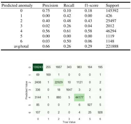
In KNN, the object is classified by a majority vote of its neighbors, and they are generally assigned to a class most common among its k nearest neighbors. A KNN with 100 neighbors and Euclidean distance as metric gives an overall accuracy of 0.95. The Precision and Recall of each classification category are shown in Table 4.

Table 4.Results for KNN.

Predicted anomaly Precision Recall f1-score Support

0 0.75 0.10 0.18 145392 1 0.00 0.42 0.00 426 2 0.40 0.48 0.43 25497 3 0.02 0.26 0.04 2012 4 0.56 0.61 0.58 46294 5 0.00 0.00 0.00 1119 6 0.03 0.50 0.06 1148 avg/total 0.66 0.26 0.29 221888

Fig. 5.Confusion matrix for predictions using KNN classifier. The first column is for benign packets (anomaly=0) and algorithm classifies 139,243 packets correctly; 6,149 flows incorrectly as result of false negatives, 3,607 flows incorrectly as result of false positives. Similarly, every column can be analyzed to check the false positives and false negatives results.

The anomaly #1 is the Bot attack and most of the records are not classified correctly. This is because we have very low number of samples that are from bot attacks. KNN is computationally expensive and has a high memory requirement. So, we also need to consider that during performance evaluation of this algorithm.

Random Forest(RF) is a popular ensemble method based on a standard machine learning technique called “decision tree”. In a decision tree, a pair of variable-value is chosen that will split in such a way to generate “best” two child subsets. Then again, the algorithm is applied on each branch of the tree. As an input enters the root of the tree and traverses down the tree and gets bucketed into smaller sets. Random forest chooses a subsample of the feature space in each split and makes the trees de-correlated.

Random forest also prunes the tree by setting a stopping criterion for the node splits. ”max features” is a parameter used to tune the maximum number of features used to split the node.

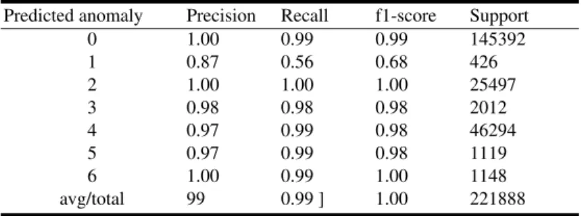
With a max features of 10 and default criteria ‘gini’ and minimum samples of leaf set to 3, an overall accuracy of 0.99 is achieved.

As seen in table 5, most of the DoS attacks are predicted accurately with random forest. The Precision is 100% on the normal and slowloris attack, and more than 90% for DoS using Golden Eye, Hulk and slowhttptest. The accuracy is much better than logistic and KNN classification algorithms.

Table 5.Results for Random Forest.

Predicted anomaly Precision Recall f1-score Support

0 1.00 0.99 0.99 145392 1 0.87 0.56 0.68 426 2 1.00 1.00 1.00 25497 3 0.98 0.98 0.98 2012 4 0.97 0.99 0.98 46294 5 0.97 0.99 0.98 1119 6 1.00 0.99 1.00 1148 avg/total 99 0.99 ] 1.00 221888

Random forest took about 1 minute and 28 seconds to run in a laptop with Intel core i7 processor. This algorithm seems to perform better even when there are low samples to train the model.

This is promising in an anomaly detection model since it may not be possible to always get the algorithm trained with lot of sample data considering new kinds of attack penetrate the internet every year so quickly. Training time of random forest is also very reasonable compared to most of the other algorithms.

Fig. 6.Confusion matrix for predictions using Random Forest. The first column is for benign packets (anomaly=0) and algorithm classifies 143,766 packets correctly; 1,626 flows incorrectly as result of false negatives, 631 flows incorrectly as result of false positives. Similarly, every column can be analyzed to check the false positives and false negatives results.

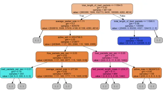
Fig. 7.Represents one of the estimators in the Random Forest Model with a depth of 4 leaves.

Figure 7 shows four levels in depth of one of the estimators to visualize the way that Random Forest make decisions based on the Gini index - measure of homogeneity in the dual partition created by each node of each tree in the forest.

Na¨ıve Bayes Classifier(NB) is based on Bayes’ theorem, with an assumption that each feature is independent from one another. When the data is continuous, the assump-tion is that the continuous values for each class are distributed according to a Gaussian distribution Na¨ıve Bayes is generally used to represent the class conditional probability for continuous attributes. That’s because, distribution is categorized by mean and vari-ance. The algorithm could not detect anything with respect to Bot and slow attacks like slowHttpTest and slowloris.

Table 6.Results for Na¨ıve Bayes.

Predicted anomaly Precision Recall f1-score Support

0 0.75 0.10 0.18 145392 1 0.00 0.42 0.00 426 2 0.40 0.48 0.43 25497 3 0.02 0.26 0.04 2012 4 0.56 0.61 0.58 46294 5 0.00 0.00 0.00 1119 6 0.03 0.50 0.06 1148 avg/ total 0.66 0.26 0.29 221888

As shown in table 6, Na¨ıve Bayes performed poorly and could not detect Bot at-tacks, DoS GoldenEye, slowloris and Slowhttptest. The accuracy on DDoS and DoS Hulk is 50% indicating that the results are pretty much random classification even on these attacks. The overall accuracy was 26% and the algorithm ran in 3.8 seconds.

Fig. 8.Confusion matrix for predictions using Na¨ıve Bayes. The first column is for benign packets (anomaly=0) and algorithm classifies 14,819 packets correctly; 130,573 flows incorrectly as result of false negatives, 4,878 flows incorrectly as result of false positives. Similarly, every column can be analyzed to check the false positives and false negatives results.

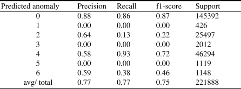
Multi-Layer Perceptron(MLP) is a class of feedforward artificial neural network model that consist of at least three layers of nodes: an input layer, a hidden layer and an output layer. Except for the input nodes, each node is a neuron that uses a nonlinear activation function. With this model we got an accuracy of 77% but the algorithm failed to detect the slow attacks and attacks with low samples of data.

Multi-Layer Perceptron also took about 6 minutes to run in a laptop with intel i7 core processor.

Table 7.Results for Multi-layer Perceptron.

Predicted anomaly Precision Recall f1-score Support

0 0.88 0.86 0.87 145392 1 0.00 0.00 0.00 426 2 0.64 0.13 0.22 25497 3 0.00 0.00 0.00 2012 4 0.58 0.93 0.72 46294 5 0.00 0.00 0.00 1119 6 0.59 0.38 0.46 1148 avg/ total 0.77 0.77 0.75 221888

Fig. 9.Confusion matrix for predictions using Multi-Layer Perceptron. The first column is for benign packets (anomaly=0) and algorithm classifies 124,957 packets correctly; 20,435 flows incorrectly as result of false negatives, 17,560 flows incorrectly as result of false positives. Simi-larly, every column can be analyzed to check the false positives and false negatives results.

Dense Neural Network(DNN) Tensorflow DNN is a Machine learning library de-veloped by Google. In tensorflow, computational graph is used to represent the flow of data. The nodes are computations and edges are data items or tensors that are n-dimensional. Each neuron will compute and transform the input data and tensors rep-resent data in a n-dimensional array. The output of each training step is fed as input to the subsequent iteration or epochs. The rank of the tensor is an integer, scalar has a zero rank, vector has rank one, matrix has rank two and so on. The shape of a tensor indicates how many elements in each dimension.

AdamOptimizer is alternate to classic stochastic gradient descent algorithm that combines Adaptive Gradient Algorithm (AdaGrad) and Root Mean Square propagation (RMSProp).

Batch Normalization - It is seen that with Batch normalization, the training speed as well as the accuracy of prediction has improved. As neural network progress, the inputs will change between each layer as the weights and biases change, so this typi-cally demands and very low learning rate to be employed to overcome saturating the model performance. With Batch normalization [21], each mini-batch that is training is normalized.

Activation Function -The activation function takes the input and transforms the in-put relation into an outin-put by adding non-linearity to the inin-puts. Some common activa-tion funcactiva-tions are Sigmoid, hyperbolic tangent(tanh), rectified linear unit and softmax. The softmax transformation is used a lot in the classification problem, softmax trans-forms a bunch of arbitrarily large or small numbers into a valid probability distribution. The output ranges from 0 to 1 and sum of all output is 1. However, a new activation function called ‘Exponential Linear Units’ (ELUs) help deep learning algorithms to gain more accuracy and speed as described in [20] by Clevert and Hochreiter. In this project, ELU is used for the network anomaly detection.

Fig. 10.Adam optimizer with dropout implemented in each layer.

Backpropagation - A forward propagation is the process of pushing the inputs through the neural network. At the end of each iteration (or epoch) the obtained outputs are compared with the targets to form the errors. Then, at the end of each epoch, the errors are back propagated and used to change the weights of each hidden layer accordingly. The back propagation helps the algorithm determine which weights contribute to which errors and adjusts the weights accordingly.

Reduce Overfitting by dropout and early stopping techniques - Dropout is a regular-ization method that refers to turning ‘off’ or ignoring some neurons during the training phase of certain iteration. In a fully connected layer, the neurons develop codependency amongst each other which will curb the individual power of each neuron leading to over-fitting of training data. In order to avoid this, dropout is generally set to a proba-bility value. Early stopping is used to avoid overfitting. One way to avoid overfitting is to train for a preset number of epochs. This is more of a Na¨ıve method. A better method is to stop when the updates in the gradient descent becomes too small. Validation test strategy is the best method where the algorithm needs to be stop when the validation loss starts to increase. Best practice is to combine validation test strategy with updates, that is the algorithm will stop when either the updates (training loss) are too small or when the validation loss starts to increase.

Initialization is a process of using a method to initialize the weights and biases. ‘He’ initialization works better for deep nets with ReLu activation and hence this method

is used, the Xavier initialization works better for deep nets with sigmoid activation. In Tensorflow by default the Xavier initializer is used, however for this project ‘He’ initialization is used.

Cross-Entropy or log loss evaluates the classification algorithm with output being a probability between 0 and 1. When the predicted probability diverges from the true value, the log loss is high. Log loss will penalize both Type-I and Type-II errors but when the prediction diverges a lot from true label, the log loss adds a high penalty.

DNN was able to detect flood based and slow DoS attacks except for the Bot attack.

Table 8.Results for Dense Neural Network.

Predicted anomaly Precision Recall f1-score Support

0 0.98 0.98 0.98 145564 1 0.00 0.00 0.00 365 2 0.99 0.99 0.99 25393 3 0.85 0.79 0.82 2076 4 0.95 0.98 0.96 46210 5 0.92 0.76 0.83 1099 6 0.85 0.81 0.83 1181 avg/ total 0.98 0.98 0.98 221888

Fig. 11.Confusion matrix for predictions using Dense Neural Network. The first column is for benign packets (anomaly=0) and algorithm classifies 142,870 packets correctly; 2,487 flows in-correctly as result of false negatives, 2,670 flows inin-correctly as result of false positives. Similarly, every column can be analyzed to check the false positives and false negatives results.

The Bot anomaly had only 0.1% of samples available for training and test. Except Random Forest all other algorithms could not detect the Bot attack with such low sam-ples. Leaving Random forest aside, compared to all other algorithms, DNN was able to predict different kinds of anomalies with reasonable accuracy. Slow DoS attacks had 95% precision and DDoS had 99% precision. DNN takes a long time to train on a regular laptop. With a dataset of 1.1 million records, DNN with 5 hidden layers and 50 neurons at each layer took 8 minutes to train. Tensorflow supports distributing the workload using GPU, future enhancement of this project should take into consideration running all models in a distributed computing environment.

Fig. 12.Validation accuracy and loss for DNN.

Figure 12 shows the output of validation loss and validation accuracy as the num-ber of iterations progress. The validation accuracy increased in the beginning and then saturates, the validation loss reduces as the number of iterations increase, the algorithm is set to stop when there is no improvement in validation loss for 20 epochs.

5

Evaluation

The evaluation of classification problem is based on the number of correct predictions on the test dataset. This is given by confusion matrix that shows the actual class label vs. the predicted class label for each category.

In data analytics, the evaluation depends not only on the standard metrics used like precision, recall, accuracy but also on the type of problem and the cost of making a mistake, in this case we are interested in the false negative predictions rate of an attack, receive a negative prediction for an attack when we should have received a positive one.

Table 9.False negative percentage for all the models covered in the research.

Anomaly Multiomial Logistic Regression K-Nearest Neighbor Random Forest

Na¨ıve Bayes Multi-Layer Perceptron Dense Neural Networks 0 2.83 4.23 1.12 89.81 14.06 1.71 1 100 60.33 43.66 57.75 100 100 2 46.14 10.08 0.12 52.03 87.05 1.09 3 74.35 18.14 1.54 73.81 100 17.97 4 15.51 4.57 0.81 38.56 7.31 3.3 5 50.67 17.16 0.80 99.91 100 20.55 6 70.99 19.16 0.96 49.91 61.65 3.47 Average 41.36 16.36 6.86 58.84 58.34 20.66

Fig. 13.False Negative percentages for all anomaly values for each performed model where the best results belong to Random Forest (RF) model. The anomaly that all the models did not predict properly was anomaly = 1 (Bot).

All the models presented were evaluated with the percentage of false negative, com-parison table 9 and figure 13.

False negatives create two problems. The first is a false sense of security. The sec-ond, more serious issue, is that potentially dangerous situations may be missed. In statis-tics, a false negative is usually called a Type II error. A false negative represents that the specific attack was not predicted when the communication is being compromised so will be missed and this might result in serious damage, so we prefer a model with good accuracy and low percentage of false negative values.

Table 10.Performed models results.

Model Overall Accuracy Overall Precision Training Time (seconds) MLR 0.88 0.89 364 KNN 0.95 0.66 63 RF 0.99 0.99 88 NB 0.26 0.66 188 MLP 0.77 0.77 116 DNN 0.97 0.98 523

Overall accuracy, precision and training time results are shown in table 10 and graphics shown in figure 14 where we can see that Random Forest (RF) has the highest accuracy and precision.

Fig. 14.Accuracy and precision for the performed models (left), Training time for the performed models (right).

The ROC (Receiver Operating Characteristics) curve is a fundamental tool used for diagnostic test evaluation. In a ROC curve the true positive rate (Sensitivity) is plot-ted in function of the false positive rate (100-Specificity) for different cut-off points of the parameter. Each point on the ROC curve represents a sensitivity/specificity pair. The accuracy of a test to discriminate normal vs anomaly case is evaluated using the

ROC curve analysis. It tells how much the model is capable of distinguishing between classes. ROC is a probability curve and AUC (Area Under the Curve) represents degree or measure of separability. AUC indicates how much the model is capable of distin-guishing between classes. ROC curve would be used to evaluate the performance of the DDoS classification model.

A classification model with perfect discrimination (no overlap between the classes) has a ROC curve that passes through the upper left corner (100% sensitivity, 100% specificity). The closer the ROC curve is to the upper left corner, the higher the overall accuracy of the classification is. Figure 15 shows ROC curve for DNN and figure 16 shows ROC curve for Random Forest. In this case there is extremely concave curve because of high prediction accuracy seen in Random Forest and DNN on most of the anomaly except the class-1 which is a ‘Bot’ attack that had only 2K packets represent-ing less than 0.2% of records in the dataset.

Fig. 15.ROC for Dense Neural Network.

When the predictions overlap, Type-I and Type-II errors are introduced. If the model predictions are 100% wrong, then the AUC is 0 and if the model predictions are 100% correct the AUC is 1.0. AUC is a classification-threshold-invariant. The ROC curves were built on truth value of ‘1’ and ‘0’. For a benign packet flow, the prediction will be ‘1’ when its predicted correctly, and ‘0’ for all other classes. This prediction from the model is plotted against the true value which is again ‘1’ or a ‘0’. This is the reason for the angle-shaped elbow seen in the ROC curve. From comparing the curves between RF and DNN it is clearly seen that RF performs very well compared to DNN on most of the classes.

6

Ethical Considerations

There are several public datasets available for anomaly detection and intrusion detec-tion research, however most of the datasets are more than a decade old and don’t take into consideration the change in the type of DDoS attacks in real network. DDoS has been a threat for a long time but the techniques to launch an attack has become easily accessible to everyone with internet access in only recent years. On the other hand, the challenge in doing research in such domain is that often these packets carry sensitive user information so organizations are not willing to publicly release packet captures from actual production network. Various ethical and practical concerns limit the access to real data. Access to datasets after anonymizing the sensitive information is needed for openness in cyber-security research but limited primarily to the organizations that generate and analyze the data.

As explained by Shou [15] there are several privacy laws that limit access to net-work traffic or address the storage of this information. In the US, the Wiretap Act [16] prohibits interception of the contents of communications, the Pen/Trap statute [18] pro-hibits real time interception of the non-content, and the Stored Communications Act [17] that prohibits providers from knowingly disclosing their customer’s communica-tions. In contrast to HIPAA [19], which restricts disclosures of health information but provides means for researchers to obtain information with and without individual con-sent, the cyber privacy laws mentioned above contain no research exceptions.

Companies often perform their research internally hiring interns from research labs to experiment on the organization’s data; in this way they maintain intellectual property rights and prevent data leakage.

Making data universally accessible after applying the right anonymization to sensi-tive information would be ideal but organizations prefer releasing synthetic data gener-ated in research labs than actual production network data. Some cybersecurity research universities generate their own data sets that resemble the true real-world data and made them publicly available for researchers.

The proposed model in this paper is based on a generated dataset available from Canadian Institute for Cybersecurity [12] that includes seven common network attacks including DoS/DDoS that met real world criteria and is publicly available for research.

7

Conclusions and Future Work

With the features derived from traffic pattern characteristics in a network, different anomalies can be detected with high accuracy. The flow based categorization of traffic and feature extraction is very useful in anomaly detection. The top flow based features that are helpful in identifying anomalies are total length of backward packets, average packet size, total length of forward packets, backward packets per second, flow duration and mean flow inter-arrival time.

Random forest model has high overall classification accuracy and low percentage of false negative predictions with an acceptable training time. Random Forest model outperforms all other algorithms for anomaly detection and can be trained in order of seconds.

The second-best model is Dense Neural Networks that is more complex in archi-tecture. Even though DNN is widely used, it took longer time for training the model to detect a DoS/DDoS attack as compared to many other algorithms and especially Random Forest.

Based on the business understanding of the problem, the false negatives have a huge impact to businesses in terms of revenue loss and brand quality. If the anomaly is not detected and mitigated on time, it could cause huge loss and reputation to the organization. A misclassification of normal packet as anomaly will impact considerably in costs, however the impact depends on the mitigation techniques applied.

In future, the model can be applied in actual network by extracting the flow based features from the network nodes. The detection engine can be a module or an applica-tion running on a centralized node that can be constantly fed with the data. The trained model can raise alarm to network admin for action when the anomaly is detected. By having the detection engine in a centralized node, the attack can be detected earlier es-pecially when the attacker is distributed in the network.

References

1. Author, Kupreev, O., Badovskaya, E., & Gutnikov, A. (2018, October 31).: Article title. DDoS Attacks in Q3 2018, from https://securelist.com/ddos-report-in-q3-2018/88617/, Re-trieved November 2018.

2. Auhor, Lloyd, A. (2018, April 23).: Article title. DDoS Attacks Can Cost Organiza-tions $50,000 Per Attack, from https://www.corero.com/blog/883-ddos-attacks-can-cost-organizations-50000-per-attack.html, Retrieved December, 2018.

3. M. Nugraha, I. Paramita, A. Musa, D. Choi, B. Cho, ”Utilizing OpenFlow and sFlow to Detect and Mitigate SYN Flooding Attack TT -”, J. KOREA Multimed. Soc., vol. 17, no. 8, pp. 988-994, Aug. 2014.

4. R. Braga, E. Mota, A. Passito, ”Lightweight DDoS flooding attack detection using NOX/OpenFlow”, Proc. - Conf. Local Comput. Networks. LCN, pp. 408-415, 2010. 5. T. Peng, C. Leckie, R. Kotagiri, Proactively detecting DDoS attack using source IP address

monitoring, in: The 3rd Int. IFIP-TC6 Networking Conf: Lecture Notes in Computer Science, vol. 3042, 2004, pp. 771–782.

6. L. Feinstein, D. Schnackenberg, R. Balupari, D. Kindred, Statistical approaches to DDoS attack detection and response, in DARPA Information Survivability Conf. and Exposition, 2003, pp. 303–314.

7. 2000 DARPA Intrusion Detection Scenario Specific Datasets. (n.d.). Retrieved Septem-ber 2018, from https://www.ll.mit.edu/r-d/datasets/2000-darpa-intrusion-detection-scenario-specific-datasets

8. DARPA 2009 Intrusion Detection Dataset. (n.d.). Retrieved September 2018, from http://www.darpa2009.netsec.colostate.edu/

9. Kokila RT, s. Thamarai Selvi, Kannan Govindarajan,”DDoS Detection and Analysis in SDN-based Environment Using Support Vector Machine Classifier”, 2014 Sixth International Con-ference on Advanced Computing(ICoAC)

10. Marwane Zekri, Said El Kafhali, Noureddine Aboutabit1 and Youssef Saadi DDoS Attack Detection using Machine Learning Techniques in Cloud Computing Environments

11. Radford, Benjamin & D Richardson, Bartley & E Davis, Shawn. (2018). Sequence Aggre-gation Rules for Anomaly Detection in Computer Network Traffic.

12. Search UNB. (n.d.). Retrieved December 2018, from https://www.unb.ca/cic/datasets/index.html

13. Iman Sharafaldin, Arash Habibi Lashkari, and Ali A. Ghorbani, “Toward Generating a New Intrusion Detection Dataset and Intrusion Traffic Characterization”, 4th International Conference on Information Systems Security and Privacy (ICISSP), Portugal, January 2018. 14. Search UNB. CIC Applications CICFlowMeter (formerly ISCXFlowMeter). Retrieved

December 2018, from https://www.unb.ca/cic/research/applications.html

15. Shou D. (2012) Ethical Considerations of Sharing Data for Cybersecurity Research. In: Danezis G., Dietrich S., Sako K. (eds) Financial Cryptography and Data Security. FC 2011. Lecture Notes in Computer Science, vol 7126. Springer, Berlin, Heidelberg.

16. 18 U.S. Code§2510 - 18 USC Ch. 119: WIRE AND ELECTRONIC COMMUNICATIONS INTERCEPTION AND

INTERCEPTION OF ORAL COMMUNICATIONS. (2002). Retrieved February 2019, from http://uscode.house.gov/view.xhtml?path=/prelim@title18/part1/chapter119&edition=prelim. 17. 18 U.S. Code§2701-2711 18 USC Ch. 121: STORED WIRE AND ELECTRONIC

COMMUNICATIONS AND TRANSACTIONAL RECORDS ACCESS. (2018). Retrieved February 2019, from

http://uscode.house.gov/view.xhtml?path=/prelim@title18/part1/chapter121&edition=prelim 18. 18 U.S. Code§3121-3127 - 18 USC Ch. 206: PEN REGISTERS AND TRAP AND

TRACE DEVICES. (2018). Retrieved February 2019, from

http://uscode.house.gov/view.xhtml?req=granuleid:USC-prelim-title18-chapter206&edition=prelim

19. HHS Office of the Secretary, Office for Civil Rights. (2018, June 13). Research. Retrieved February 2019, from

https://www.hhs.gov/hipaa/for-professionals/special-topics/research/index.html

20. Clevert, Djork-Arn´e, Unterthiner, Thomas, Hochreiter, & Sepp. (2016, February 22). Fast and Accurate Deep Network Learning by Exponential Linear Units (ELUs). Retrieved February 2019, from https://arxiv.org/abs/1511.07289

21. Ioffe, S., & Szegedy, C. (2015, March 02). Batch Normalization: Accelerating Deep Network Training by Reducing Internal Covariate Shift. Retrieved February 2019, from https://arxiv.org/abs/1502.03167