Digital Divide: An Econometric Study of the Determinants in Information-poor Countries

(1)

Digital Divide: An Econometric Study of the

Determinants in Information-poor Countries

TASNEEM ZAFAR and KHALID AFTAB

*

There can not be two opinions on the importance of Information and Communication Technology (ICT) for economic development. However, real disparities exist in access to and use of ICT across countries. The digital divide is a complicated matter of varying levels of access, basic usage, and applications of ICT among countries and peoples. Using the Gompertz Technology Diffusion model, this paper attempts to measure the contribution of factors such as affordability, knowledge, infrastructure, human capital, trade openness, and economic and social environment in the technology diffusion process, specially in the case of information-poor countries.

JEL classification: O33, L96

Keywords: Digital Divide, Information and Communication Technologies, ICT,

Gompertz Model, ICT Diffusion, Economic Development, ICT

Infrastructure

I. INTRODUCTION

The need for access to Information and Communication Technology (ICT) for

accelerated economic development has increased manifold in the information age. Not

only are the new technologies considered a key to unlocking economic growth, they

impinge on and can impact virtually all aspects of development. In this regard, a number

of well-known declarations concerning developmental applications of Information and

Communication Technology (ICT) rest on the experiences of high- or middle-income

countries, and are simply assumed to be valid in other settings as well.

With its power to influence profoundly every sector of the economy, improved

access to information and communications is central to improving the lives of people in

the third world. And institutions in these countries, ranging from public bureaucracies

and large enterprises, to small businesses and NGOs have the obvious need to improve

their efficiency and effectiveness through access to modern means of communication i.e.

computers, basic software and internet. All of this and much more, would be done if there

were no constraints (or relatively malleable constraints) on governments, communities

and individuals attempting to improve the quality of life in the developing world—just as

it has been done in the advanced industrial world. However, there are extremely serious

constraints on using ICT to improve the lot of most people in the Third World. These

constraints are only partially technical and to a greater extent, they are economic, social

and political. They flow not only from unresolved problems of poverty and economic

inequality in particular countries and regions, but also from the structure and dynamics of

Tasneem Zafar <[email protected]> is Lecturer in Economics and Khalid Aftab <[email protected]> is Professor of Economics at GC University, Lahore.

(2)

the global economic system. Furthermore, whatever efforts are made to improve access to

ICT in these countries, these take place within extremely varied cultures and social

structures which shape the outcome of technological change in particular ways. Both the

need for certain ICT products and their use may, thus, differ markedly from what might

be expected in advanced industrial societies.

Thus far the gains of the digital revolution have been confined to a comparatively

small group of countries, mainly in the industrialised world. The unequal distribution of

the new and old the ICT across countries and associated efficiency gains go by the name

of Digital Divide. It is the logical consequence of the social and economic imbalances

that already exist within and across the countries. Although broadening of physical access

to information and communication technologies is often a necessary step in reducing the

digital divide, it is almost never sufficient to do so because the problem goes beyond the

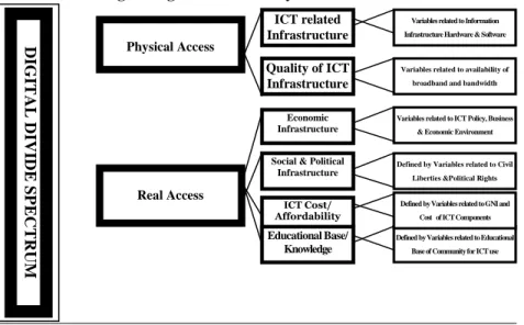
physical access and is related to real access. Physical access is determined by the

availability of ICT related to infrastructure and its quality. But ‘Real Access’ is

determined by: affordability; knowledge; IT training; its usage; human capital;

sociopolitical conditions; and economic infrastructure available in a country.

Section I introduces the problem and gives the analytical framework used in the

papers. Section II details the methodology. Section III describes the variables included in

the study in the light of the literature review. This section also analyses the data sources.

Section IV reports empirical findings of the study, and Section V summarises the findings

of the study.

Figure 1 below throws light on the digital divide spectrum.

Fig. 1. Digital Divide Analytical Framework

A glance at Figure 1 shows the presence of two sets of physical and real factors

which influence countries access to ICT. We use this framework to place different

information poor countries along Digital Access Index (DAI) ranking scale across

countries. This is shown in Table 1.

Physical Access

Quality of ICT Infrastructure

Economic Infrastructure

Social & Political Infrastructure ICT Cost/ Affordability Educational Base/ Knowledge Real Access

D

IG

IT

A

L

D

IV

ID

E

S

P

E

C

T

R

U

M

Variables related to availability of broadband and bandwidth

Variables related to ICT Policy, Business & Economic Environment

Defined by Variables related to Educational Base of Community for ICT use Defined by Variables related to GNI and

Cost of ICT Components Defined by Variables related to Civil

Liberties &Political Rights ICT related

Infrastructure

Variables related to Information Infrastructure Hardware & Software

(3)

Table 1

‘Information-poor Countries’ included in Analysis with Digital Access Index (DAI) Score

Less than or Equal to 0.37 out of 1

African Countries

Country Score Country Score Country Score Country Score Algeria 0.37 Djibouti 0.15 Madagascar 0.15 Sudan 0.13

Benin 0.12 Egypt 0.40 Malawi 0.15 Tanzania 0.15

Burkina Faso 0.08 Equatorial Guinea 0.20 Mali 0.09 Uganda 0.17 Burundi 0.10 Ethiopia 0.10 Mauritania 0.14 Zambia 0.17 Cameroon 0.16 Gambia 0.13 Mozambique 0.12 Zimbabwe 0.29 Central African Rep. 0.10 Ghana 0.16 Nepal 0.19

Chad 0.10 Guinea 0.10 Niger 0.04

Comoros 0.13 Guinea-Bissau 0.10 Nigeria 0.15

Congo 0.17 Kenya 0.19 Rwanda 0.15

Côte d'Ivoire 0.13 Lesotho 0.19 Senegal 0.14

Asian Countries Armenia 0.30 Pakistan 0.24 Azerbaijan 0.24 Syria 0.28 Bangladesh 0.18 Tajikistan 0.21 Bhutan 0.13 Turkmenistan 0.37 Cambodia 0.17 Uzbekistan 0.31 Georgia 0.37 Viet Nam 0.31

India 0.32 Indonesia 0.34 Kyrgyzstan 0.32 Lao P.D.R. 0.15 American Countries Haiti 0.15 Honduras 0.29 Nicaragua 0.19 European Country Moldova 0.37 Oceania

Papua New Guinea 0.26

Source: International Telecommunication Indicators 1998–2003.

Note: Scores are on a scale of 0 to 1 where 1 = highest access and 0 = lowest score. DAI values are shown to

hundreds of a decimal point. Countries with the same DAI value are ranked by thousands of a decimal point by ITI.

Because of considerable differences in physical and real access across countries, it

would be important to estimate the relative significance of various determinants of digital

divide. This should help in identifying the factors that shape the environment in which

modern ICT get diffused into the economies and what makes particular applications and

services useful, especially in the case of information poor countries.

(4)

II. METHODOLOGY

Using Gompertz Technology Diffusion model, this study estimates factors that are

responsible for the slow technology diffusion process in the information poor countries. This

kind of model was used by [Stoneman (1983)] for modeling spread of computers. The

specifications of the model are as follows:

T

it

is an indicator of Information and Communication Technology (ICT) in a

country

_i

in year ‘t’ and

T be its post diffusion or equilibrium level or value (

_i*

T or

_i*

equilibrium level of ICT in country ‘i’ will be a function of exogenous demand side

variables).

Most of the models of technology of technology adoption assume that over time

it

T tends to

T along an S-shaped path i.e. this model assumes that spread between the

i*

value of the ICT indicator in year ‘t’ and its value in year ‘t–1 ‘is a function of the spread

between a target value (or post diffusion value)

T

*

and value in year t–1.

1 *

1

(ln

ln

T

it

−

T

it₋

=

α

i

T

i

−

T

it₋

)

…

(1)

Where

α

i

is the speed of adjustment taken to be constant in our analysis.

Moreover we assume that most of the explanatory variables change over time. We

may say that T

i*

is time dependent and express it as:

it it i io it

Y

Z

T

=

β

+

β

ln

+

γ′

ln

1 *

…

(2)

where post diffusion level of technology is a function of

Y

_it

, i.e. the national income of

the country ‘i’ in year ‘t’ and

Z

_it

, which is the vector of other possible variables

describing the demand or supply conditions e.g. infrastructure, openness to international

trade, economic freedom, knowledge or educational base of country ‘

i

’ in year ‘t’.

The estimable equation is obtained by inserting (2) in to (1).

ε

+

α

−

γ′

α

+

β

α

+

β

α

=

−

ln

−1 1

ln

−1

ln

T

_it

T

_it _i _o _i _i

Y

_it _i

Z

_it _i

T

_it

…

(3)

where

ε

is a white noise i.e. where the error terms are uncorrelated with zero mean and

σ

2

variance.

III. DESCRIPTION OF THE VARIABLES

AND DATA SOURCES

The estimates of Gompertz Technology Diffusion model are reported in Section

IV of this research paper for four ICT indicators i.e. cellular mobile subscribers per 100

inhabitants, personal computers per 100 inhabitants, internet hosts per 10,000 inhabitants,

and internet users per 10,000 inhabitants. The data on these variables are for the period

1998–2003. The first three variables are taken as indicators of the state of the ICT

infrastructure, so they will help to study the diffusion process of ICT infrastructure, while

the fourth indicator, internet users, measures access to the internet. It is worth noting that

the difference between communication technology and information technology has

become blurred. For example, mobile phones are primarily tools of communication, but

with the advent of wireless applications, consumers can access data and information via

(5)

cellular phone. The internet is mainly an indicator of information technology, yet, many

internet users communicate with other users from their personal computers. Thus, all

three information indicators: internet hosts, internet users and personal computers have

also become tools of communication.

The first explanatory variable in estimable equation is Gross National Income

(GNI) per capita measured in international dollars. This variable is included to capture

affordability. GNI is converted to international dollars using purchasing power parity

rates. An international dollar has the same purchasing power over GNI as a U.S. dollar

has in United States. Purchasing power parity (PPP) rates provide a standard measure

allowing comparison of real price levels between countries, just as conventional price

indices allow comparison of real values over time. Data for GNI is taken from world

development indicators database, 2003. Historical data from developed nations indicate

that adoption and diffusion of ICT is highly correlated with income. Countries with

higher per capita income invest more in research and development and, hence, are more

able to discover and use advanced information technologies. Prior to the spread of the

internet, fixed telephones Hardy (1980) and telephone infrastructure Norton (1992) were

used to model communication effects on economic growth. Since mid-1990s however

other indicators of ICT began to be emphasised and more robust econometric tests are

being employed. In general, the association between ICT and income is expected to be

strong and positive.

The first variable in vector ‘Z’ is education. Low levels of education and literacy

are expected to hinder both real accessibility and dissemination of ICT. Since the use of

knowledge-based products requires a basic level of literacy, we would expect to see

higher education causing higher ICT use and its consumption. Diffusion of ICT may

require higher or tertiary education, and scientific research. Kiiski and Pohjola (2002)

showed that, in a sample including developing and OECD countries, tertiary education

had a positive and statistically significant influence on ICT diffusion. In contrast,

Hargittai (1999), and Kiiski and Pohjola (2002) have found that in the case of industrial

countries, education did not seem to influence ICT diffusion. These conflicting results

suggest that this can be an important explanatory variable and need to be empirically

tested. Also, in a sample that included both developed and developing countries, Norris

(2000) shows that education did not have a significant influence on ICT diffusion.

Consistent data on tertiary education are not available for all the countries in the sample.

This study uses adult literacy and the education index instead. This index is also used by

UNDP in generating the human development index (HDI).

This study uses three freedom indicators, which in fact represent the economic,

social and political infrastructure in the economy that create an environment conducive

for the spread of modern technologies i.e. ICT. The first indicator is the index of

economic freedom published by the Heritage Foundation. This index is an average score

of 10 indexes measured on a one-to-five scale, with 5 indicating the highest level of

economic freedom. The 10 indexes assess trade policy, monetary policy, capital flows

and foreign investment, wage and price control, banking and financial regulations,

intellectual property and black markets, property rights, regulation, transparency and

bureaucracy, government intervention in the economy, and the fiscal burden of the

government (taxes and government expenditure). At least in cross-sectional analyses,

(6)

greater (higher index) economic freedom is expected to be associated with higher GDP,

higher levels of education or literacy rates, and stronger ICT indicators.

The other freedom indicators are the index of political rights and the index of civil

liberties. By including these indices, we follow the work of Norris (2000) and try to

explore whether countries with higher levels of civil and political freedom could also

have greater ICT diffusion. These two indexes are measured on a one-to-seven scale,

with 7 indicating the highest degree of freedom. The correlation between these indices

and income is expected to be positive.

The other variables included in vector ‘Z’ are trade policy indicators. Openness to

international trade is one of two trade policy indicators used in this study. It is measured

as the ratio of the sum of exports and imports to GDP in world prices. The role of trade

policy is important. For example, Jussawalla (1999) claims that East Asian nations

fostered ICT production through openness and export-oriented investments. Both exports

and imports may offer a channel for increased adoption and diffusion of ICT. Some

imported goods and services require the existence of specific ICT to be operational. In

some cases, ICT may be embodied in the imported products. Similarly, to enhance their

exports, firms find it increasingly necessary to make use of ICT. Mobile phones, internet

use, computerized operations are all tools used to improve the efficiency of conducting

business in the global market. These tools tend to reduce the level of imperfect

information and incomplete markets. As argued by Stiglitz (1989), imperfect information

results in less trade. Thus, we would expect a positive and significant correlation between

ICT and openness to international trade. The second international trade variable is

foreign direct investment (FDI). Inward FDI usually allows recipient economies’ access

to advanced technologies, managerial skills and higher level of know-how. Transnational

corporations tend to standardise their operations around the world and train workers in

host countries according to their skill standards, including the use of ICT. Moreover, FDI

may replace ICT as a medium for information and knowledge diffusion in cases where

information and knowledge associated with ICT have a proprietary feature. As

emphasised by Bedi (1999), ‘...in such cases, the role of ICT in enabling access is

limited, and other measures such as trade and foreign direct investment may be

appropriate conduits for disseminating information and knowledge’. Thus, it is

reasonable to expect higher inward FDI to contribute to ICT diffusion.

Other variables which have been emphasised in the literature as potential

determinants of ICT diffusion include knowledge of English language Kiiski and Pohjola

(2002), income distribution [Bedi (1999); Hargittai (1999) and Pohjola (2000)], and

competition in the telecommunication industry [Hargittai (1999); Jayakar (1999); and

Kiiski and Pohjola (2002)]. The empirical evidence on the impact of these variables,

particularly in developing countries, is ambiguous or more in support of their

insignificance. So, they are not included as explanatory variables.

IV. EMPIRICAL RESULTS

The results from the linear estimation of Gompertz Technology Diffusion model

exploring the factors that influence ICT diffusion are reported in Tables 2–5. To test the

robustness of the model, four equations were estimated. As mentioned earlier, the use of

ICT in an economy can be seen through four indicators i.e. internet users, internet hosts,

(7)

number of personal computers and mobile phone subscribers. Table 2 displays the

statistical results from estimating the model with internet use as the relevant ICT variable.

Table 3 reports the findings when personal computers were the relevant ICT indicator.

Tables 4 and 5 report the results associated with internet hosts, and mobile phones,

respectively.

Equations /columns (1) and (2) in each table differ in terms of right hand side

variables because in each table (except internet hosts) the first equation reports the

findings about those right hand side variables selected as a result of stepwise model

selection procedure from all entered variables. Here one thing is worth mentioning that

the selected model in above mentioned three cases as a result of stepwise

selection

Table 2

Estimates of the Gompertz Technology Diffusion Model

Cross-section Results for Countries with DRI Score Less than or Equal to 0.4

Dependent Variable (Internet Users) ln U2 – ln U98

(1) (2)

Speed of Diffusion 0.718*** 0.780***

(0.070) (0.072)

Constant αβ0 –3.918** –4.267**

(1.943) (1.947)

GNI per Capita αβ1 0.549*** 0.491***

(0.200) (0.202) Adult Literacy

Secondary and Tertiary Education

Education Index 1.097** (0.573) Civil Liberties 0.06347 (0.057) Economic Freedom 0.08149 (0.071) Foreign Direct Investment

Openness to International Trade 0.567*** 0.383**

(0.172) (0.185)

Personal Computers -98 0.163*

(0.097)

Internet Access Cost –0.295*** –0.230**

(0.109) (0.113) F-Test 32.163*** 18.450*** R 0.879 0.902 R2 _0.772 _0.813 Adjusted R2 0.748 0.769 Number of Observations 42 42

Note: Standard errors are in parentheses.* =Significant at (0.10), i.e., at 10 percent, **=Significant at (0.05),

(8)

Table 3

Cross-section Results for Countries with DRI Score Less than or Equal to 0.4

Dependent Variable (Personal Computers) lnPCs02−lnPCs98

(1) (2) Speed of Diffusion α 0.810*** (0.115) 0.804*** (0.118) Constant αβ0 –4.734*** (1.526) –3.991*** (1.507)

GNI per Capita αβ0 0.561***

(0.184) 0.537*** (0.189 Adult Literacy 0.01483*** (0.005) 0.01311*** (0.005) Secondary and Tertiary Education

Education Index Political Rights Civil Liberties

Economic Freedom 0.155**

(0.088) Foreign Direct Investment

Openness to International Trade

Personal Computers -98 0.334***

(0.087) Internet Access Cost

F- Test 13.935*** 15.748***

R 0.812 0.794

R2 0.659 0.630

Adjusted R2 _0.612 _0.600

Number of Observations 41 41

i.e., at 5 percent and ***=Significant at (0.o1, i.e., at 1 percent.

Table 4

Cross-section Results for Countries with DRI Scores Less than or Equal to 0.4

Dependent Variable Internet Hosts (lnH02−lnH98)

Speed of Diffusion α 0.379***

(0.139)

Constant αβ0 –6.659***

(2.484)

GNI per Capita αβ1 0.889***

(0.291) Economic Freedom 0.295*** (0.166) F- Test 4.068*** R 0.508 R2 _0.259 Adjusted R2 _0.200 Number of Observations 38

(9)

Table 5

Cross-section Results for Countries with Low DRI Scores Less than or Equal to 0.4

Dependent Variable Mobile Phones (lnM02−lnM98)

(1) (2) Speed of Diffusionα –0.330 (0.908) –1.958 (1.768) Constant αβ_o 0.400*** (0.086) 0.455*** (0.099)

GNI per Capita αβ1

0.217 (0.203)

Openness to International Trade 0.573**

(0.264) 0.549** (0.265 F- Test 11.677*** 8.191*** R 0.560 0.574 2 R 0.314 0.330 AdjustedR 2 0.287 0.289 Number of Observations 53 53

Note: Standard errors are in parentheses.* =Significant at (0.10), i.e., at 10 percent, **=Significant at (0.05), i.e., at

5 percent and ***=Significant at (0.01), i.e., at 1 percent. (This should be cleared.)

procedure is also consistent with the model selected through forward selection procedure

i.e. the both methods select the same explanatory variables. Equation (2) provides the

estimates of the model including those explanatory variables selected as a result of

backward model selection procedure. Moreover all the four estimated equations satisfy

the basic assumptions of linear models as all have been duly checked (checking includes

co-linearity diagnostic through VIF(variance inflate factor), and autocorrelation through

Durbin-Watson test.

The underlying assumption here is that the diffusion process is the same in all countries

i.e. the parameter values of Gompertz Technology Diffusion model take the same value for all

‘i’ or countries, moreover the speed of diffusion is assumed to be constant over time. However

it would be more appropriate to make it time dependent as suggested by Kiiski and Pohjola

(2002), but in order to make the analysis simple it is assumed so.

Table 2 displays the statistical results of internet use as the relevant ICT indicator.

The empirical results indicate that in case of internet users both of the equations show

that model adequately captures the diffusion process since the speed of diffusion or

adjustment (coefficient on the lagged value of this variable) is highly significant in both

cases. Speed of diffusion is 0.718 in case of Equation (1) and 0.780 in case of Equation

(2) and in both cases significant at 99 percent confidence level. Moreover income,

education, openness to international trade, stock of personal computers and internet

access cost turn out to be highly significant i.e. at 99 percent confidence level in both

equations. However civil liberties and economic freedom come up with correct signs, but

are not as significant explanatory variables. If we make a comparison of two selected

models, the model selected through backward selection procedure (Equation 2) is a little

better than one selected through stepwise procedure (Equation 1) as it slightly improves

the value of adjusted R-squared i.e. from 0.75 in Equation (1) to 0.77 in Equation (2).

(10)

Table 3 displays the results of the model where ICT is represented by the number

of personal computers per 100 inhabitants. Again in this case the speed of diffusion (

α

) is

highly significant in both the selected models as it is 0.180 in case of Equation (1), and

0.804 in the case of Equation (2) and is significant at 99 percent confidence level. In the

case of internet users income, adult literacy, economic freedom, internet users turn out to

be highly significant at 99 percent confidence level. Moreover out of the two models

selected through two different selection procedures, Equation (1) is more appropriate i.e.

selected through stepwise and forward selection procedures as it gives slightly improved

value of R-square (i.e. 0.612) as compared to 0.6 in the case of Equation (1).

Table 4 displays the results when internet hosts was the ICT indicator in an

economy or dependent variable. Although the speed of diffusion is significant at 99

percent confidence level in the selected model but the value of R-square is very low.

However the results suggest that income and economic freedom are other important

significant explanatory variables that too are significant at 99 percent confidence level.

Moreover model fails to provide support for the influence of education or literacy on

internet host diffusion.

Finally, Table 5 reports the findings when mobile phone is an indicator of ICT.

Again in this case speed of diffusion adjustment is significant at 99 percent level of

confidence, but model captures weakly the diffusion process because here again the value

of adjusted R-square is low. Moreover, this is the only ICT indicator where income does

not come out to be significant. The only significant variable is openness to international

trade which is significant at 95 percent level of confidence.

In summary, the empirical results provide support for the role of income as a

major determinant of ICT diffusion because it comes out to be significant at 99 percent

confidence level in the case of internet use, internet hosts and personal computers. This is

consistent with the conclusions in Niininen (2001), Hargittai (1999), Quah (2001), Norris

(2000), and Kiiski and Pohjola (2002). Thus showing that adoption and diffusion of

modern information and communication technology is highly correlated with income

level. Countries with higher per capita income invest more in research and development

therefore are able to acquire and use advanced information technologies.

In addition, education and literacy, especially adult literacy, appears to have direct

impact on dissemination and personal computers, thus showing that education influences

technology adoption. However we do not find evidence that education is a significant

explanatory variable of mobile phone use. This may be due to the reason that use of

mobile phones does not need as much educational or training skills as it is required in

case of computer or internet use. Undoubtedly education must have a role in diffusion of

information and communication technologies for at least two reasons. Firstly, education

directly contributes to basic literacy and reading and writing skills which are essential in

use of modern ICT as knowledge-based products. More educated people are likely to be

quicker to adopt new innovations than people with less education. Secondly, based on the

facts that the early users of the internet were people working in higher education and

research academic institutions may play an important role in spreading of ICT. However,

our findings that education is important in technology dissemination is consistent with the

earlier findings of Barrow and Lee (2000) and Duncombe (2000), Caselli and Coleman

(2001) and Wong (2001) and is in sharp contrast with the findings of Hargittai (1999) and

(11)

Norris(2000), as they concluded that education is not important in technology

dissemination.

It is surprising to find that there is no support for the influence of FDI on ICT

diffusion. As mentioned earlier, FDI is an important channel through which technology

enters a country and gets disseminated. Perhaps, there is a threshold that most developing

countries in the sample have not yet reached or that FDI in the countries under study

targets labour-intensive sectors that require negligible levels of ICT. In fact, since FDI is

accounted for in the index of economic freedom, the findings do not necessarily imply

that this variable has no impact on ICT diffusion.

Moreover, the estimation yields values for the speed of diffusion adjustment (

α

)

that are consistent with the increased adoption of ICT. In a cross-sectional model

including 75 developed and developing countries, Kiiski and Pohjola (2002) report values

for the speed of diffusion that range from 0.186 to 0.527. However the empirical results

in this research paper find that the speed of diffusion can vary from 0.400 to 0.455 for

mobile phones, from 0.804 to 0.810 for personal computers and from 0.718 to 0.780 for

internet use. However, given that the RHS variables are not the same, it is difficult to

make a more meaningful comparison of the results derived in the two studies.

V. SUMMARY

This study has six important findings. First, income is a major determinant of ICT

diffusion. Income influences both ICT infrastructure as it is shown to cause higher

internet use, use of personal computers and internet hosts and access to ICT since it has

an effect on internet use. Second, there is a positive impact of government trade policies

on ICT. Openness fosters the adopting and adapting of technology. Third, at least in the

case of two ICT indicators (mobile phones and internet hosts) political rights and civil

liberties have a strong influence. Fourth, there is evidence supporting that education

(literacy) has a positive impact on ICT diffusion. Moreover, the above conclusions

highlight the role of demand in the market for knowledge-based products, and are

consistent with the propositions in Quah (2001). It is important to note that for mobile

phones openness to international trade and for internet hosts, economic freedom are

important factors, while GNI does not seem to have an effect on mobile phones.

In addition, the speed of diffusion in the case of Internet users and Personal

computers is shown to be much higher than in the case of internet hosts and mobile

phones. This finding may reflect the recent trend in large cities where cyber cafés are

mushrooming. However, it is feared that a faster diffusion of internet users (relative to

internet hosts) may lead to saturation and poor access to information. The present

findings seem to provide elements for hope and concern at the same time. On the one

hand, there is evidence through earlier researches that ICT enhances income, and hence,

it can provide an additional source of economic growth. Due to its pervasive nature, ICT

diffusion may allow a leapfrogging process to occur. On the other hand, the finding that

trade policies and social development variables are important determinants of ICT

diffusion, as well as economic development, implies that countries with poor

performance in these variables may sink even further in the information-poor and

non-communicating side of the digital divide.

(12)

Notes: Information-poor countries considered in this research paper for the

purpose of analysis are low-access economies, i.e., the countries have a score value of

less than 0.37 according to the Digital Access Index (DAI) of ITU, 2002-03. A complete

list of these countries along with their scores can be seen in Table 1. Countries in this

category are the poorest in the world and most are LDCs. They have a minimal level of

access to the information society. The Digital Access Index (DAI) measures the overall

ability of individuals in a country to access and use information and communication

technologies. The DAI combines eight variables, covering five areas, to provide an

overall country score. The results of the Index point to potential stumbling blocks in ICT

adoption.

(13)

APPENDIX

Mathematical Derivation of Results

Details of Model Selection Procedure When Internet Users Are the Relevant

n ICT Indicator

Variables Entered / Removed (a)

Model Variables

Entered

Variables Removed

Method

1 LN-USERS-98 . Stepwise (Criteria: Probability-of-F-to-enter <=

.050, Probability-of-F-to-remove >= .100).

2 LN-Avg GNI . Stepwise (Criteria: Probability-of-F-to-enter <=

3 ln-OPEN . Stepwise (Criteria: Probability-of-F-to-enter <=

4 ln_internet tariff . Stepwise (Criteria: Probability-of-F-to-enter <=

.050, Probability-of-F-to-remove >= .100). (a) Dependent Variable: USERs (LN02-98).

Model Summary

Model R R Square Adjusted R Square Std. Error of the Estimate

1 .525(a) .276 .258 .89848688218940

2 .818(b) .669 .652 .61554392824644

3 .853(c) .728 .707 .56438514885354

4 .879(d) .772 .748 .52380532999675

(a) Predictors: (Constant), LN-USERS-98.

(b) Predictors: (Constant), LN-USERS-98, LN-Avg GNI.

(c) Predictors: (Constant), LN-USERS-98, LN-Avg GNI, ln-OPEN.

(d) Predictors: (Constant), LN-USERS-98, LN-Avg GNI, ln-OPEN, ln_internet tariff.

ANOVA(e)

Model

Sum of Squares

df

Mean Square

F

Sig.

Regression

12.626

1

12.626

15.640

.000(a)

Residual

33.098

41

.807

1

Total

45.724

42

Regression

30.569

2

15.284

40.339

.000(b)

Residual

15.156

40

.379

2

Total

45.724

42

Regression

33.302

3

11.101

34.849

.000(c)

Residual

12.423

39

.319

3

Total

45.724

42

Regression

35.298

4

8.825

32.163

.000(d)

Residual

10.426

38

.274

4

Total

45.724

42

(b) Predictors: (Constant), LN-USERS-98, LN-Avg GNI. (c) Predictors: (Constant), LN-USERS-98, LN-Avg GNI, ln-OPEN.

(d) Predictors: (Constant), LN-USERS-98, LN-Avg GNI, ln-OPEN, ln_internet tariff. (e) Dependent Variable: USERs (LN02-98).

(14)

Coefficients (a) Unstandardised

Coefficients

Standardised Coefficients

Model B Std. Error Beta t Sig.

(Constant) 1.708 .351 4.869 .000 1 LN-USERS-98 –.411 .104 –.525 –3.955 .000 (Constant) –6.780 1.257 –5.396 .000 LN-USERS-98 –.671 .081 –.858 –8.323 .000 2 LN-Avg GNI 1.022 .149 .709 6.882 .000 (Constant) –8.138 1.242 –6.553 .000 LN-USERS-98 –.679 .074 –.868 –9.186 .000 LN-Avg GNI .963 .138 .668 6.997 .000 3 ln-OPEN .541 .185 .249 2.929 .006 (Constant) –3.918 1.943 –2.016 .051 LN-USERS-98 –.718 .070 –.918 –10.241 .000 LN-Avg GNI .549 .200 .381 2.745 .009 ln-OPEN .567 .172 .261 3.307 .002 4 ln_internet tariff –.295 .109 –.376 –2.698 .010

(a) Dependent Variable: USERs (LN02-98).

Excluded Variables (e)

Collinearity Statistics

Model Beta In t Sig.

Partial

Correlation Tolerance

LN-PCs-98 .533(a) 4.388 .000 .570 .827

LN-Avg GNI .709(a) 6.882 .000 .736 .781

CL-c –.196(a) –1.494 .143 –.230 1.000

ECF-c –.079(a) –.589 .559 –.093 .991

ln-fdi .378(a) 2.996 .005 .428 .928

ln-OPEN .336(a) 2.693 .010 .392 .985

ln_internet tariff –.694(a) –6.423 .000 –.713 .762

1

Education index .520(a) 4.212 .000 .554 .823

LN-PCs-98 .274(b) 2.592 .013 .383 .651 CL-c .048(b) .487 .629 .078 .857 ECF-c .011(b) .117 .908 .019 .970 ln-fdi .120(b) 1.147 .259 .181 .755 ln-OPEN .249(b) 2.929 .006 .425 .964 ln_internet tariff –.349(b) –2.240 .031 –.338 .311 2 Education index .265(b) 2.520 .016 .374 .660 LN-PCs-98 .225(c) 2.242 .031 .342 .628 CL-c .037(c) .410 .684 .066 .855 ECF-c .039(c) .451 .655 .073 .959 ln-fdi .124(c) 1.299 .202 .206 .755 ln_internet tariff –.376(c) –2.698 .010 –.401 .310 3 Education index .177(c) 1.632 .111 .256 .567 LN-PCs-98 .160(d) 1.588 .121 .253 .571 CL-c .030(d) .357 .723 .059 .854 ECF-c .075(d) .931 .358 .151 .934 ln-fdi .065(d) .693 .493 .113 .702 4 Education index .148(d) 1.448 .156 .232 .560

(a) Predictors in the Model: (Constant), LN-USERS-98.

(b) Predictors in the Model: (Constant), LN-USERS-98, LN-Avg GNI. (c) Predictors in the Model: (Constant), LN-USERS-98, LN-Avg GNI, ln-OPEN.

(d) Predictors in the Model: (Constant), LN-USERS-98, LN-Avg GNI, ln-OPEN, ln_internet tariff. (e) Dependent Variable: USERs (LN02-98).

(15)

Variables Entered / Removed (b)

Model Variables Entered

Variables

Removed Method

1 Education index, ECF-c, CL-c, ln-fdi,

ln-OPEN, LN-PCs-98, LN-USERS-98, LN-Avg GNI, ln_internet tariff(a)

. Enter

2 . ln-fdi Backward (criterion: Probability of

F-to-remove >= .100).

3 . CL-c Backward (criterion: Probability of

4 . ECF-c Backward (criterion: Probability of

5 . Education

Index

Backward (criterion: Probability of F-to-remove >= .100).

6 . LN-PCs-98 Backward (criterion: Probability of

F-to-remove >= .100). (a) All requested variables entered.

(b) Dependent Variable: USERs (LN02-98).

Model Summary

Model R R-Square Adjusted R Square Std. Error of the Estimate

1 .904(a) .816 .766 .50435849610735 2 .902(b) .813 .769 .50178824801358 3 .898(c) .806 .767 .50357515882357 4 .894(d) .798 .765 .50591094508067 5 .887(e) .787 .758 .51361817779732 6 .879(f) .772 .748 .52380532999675

(a) Predictors: (Constant), Education index, ECF-c, CL-c, ln-fdi, ln-OPEN, PCs-98, USERS-98, LN-Avg GNI, ln_internet tariff.

(b) Predictors: (Constant), Education index, ECF-c, CL-c, ln-OPEN, LN-PCs-98, LN-USERS-98, LN-Avg GNI, ln_internet tariff.

(c) Predictors: (Constant), Education index, ECF-c, ln-OPEN, LN-PCs-98, LN-USERS-98, LN-Avg GNI, ln_internet tariff.

(d) Predictors: (Constant), Education index, ln-OPEN, LN-PCs-98, LN-USERS-98, LN-Avg GNI, ln_internet tariff.

(e) Predictors: (Constant), ln-OPEN, LN-PCs-98, LN-USERS-98, LN-Avg GNI, ln_internet tariff. (f) Predictors: (Constant), ln-OPEN, LN-USERS-98, LN-Avg GNI, ln_internet tariff.

(16)

ANOVA (g)

Model

Sum of

Squares

df

Mean

Square

F

Sig.

Regression

37.330

9

4.148

16.306

.000(a)

Residual

8.394

33

.254

1

Total

45.724

42

Regression

37.163

8

4.645

18.450

.000(b)

Residual

8.561

34

.252

2

Total

45.724

42

Regression

36.849

7

5.264

20.759

.000(c)

Residual

8.876

35

.254

3

Total

45.724

42

Regression

36.510

6

6.085

23.775

.000(d)

Residual

9.214

36

.256

4

Total

45.724

42

Regression

35.964

5

7.193

27.265

.000(e)

Residual

9.761

37

.264

5

Total

45.724

42

Regression

35.298

4

8.825

32.163

.000(f)

Residual

10.426

38

.274

6

Total

45.724

42

(a) Predictors: (Constant), Education index, ECF-c, CL-c, ln-fdi, ln-OPEN, PCs-98, USERS-98, LN-Avg GNI, ln_internet tariff.

(b) Predictors: (Constant), Education index, ECF-c, CL-c, ln-OPEN, LN-PCs-98, LN-USERS-98, LN-Avg GNI, ln_internet tariff.

(c) Predictors: (Constant), Education index, ECF-c, ln-OPEN, LN-PCs-98, LN-USERS-98, LN-Avg GNI, ln_internet tariff.

(d) Predictors: (Constant), Education index, ln-OPEN, LN-PCs-98, LN-USERS-98, LN-Avg GNI, ln_internet tariff.

(e) Predictors: (Constant), ln-OPEN, LN-PCs-98, LN-USERS-98, LN-Avg GNI, ln_internet tariff. (f) Predictors: (Constant), ln-OPEN, LN-USERS-98, LN-Avg GNI, ln_internet tariff.

(17)

Coefficients (a)

Unstandardised Coefficients

(Constant) -4.366 1.961 –2.227 .033 LN-PCs-98 .183 .101 .188 1.811 .079 LN-Avg GNI .472 .204 .327 2.309 .027 CL-c 5.910E-02 .057 .088 1.031 .310 ECF-c 7.594E-02 .071 .085 1.066 .294 ln-fdi 4.281E-02 .053 .075 .809 .424 ln-OPEN .383 .186 .176 2.063 .047 ln_internet tariff –.199 .119 –.254 –1.668 .105 LN-USERS-98 –.779 .072 –.995 –10.755 .000 1 Education index 1.034 .581 .190 1.781 .084 (Constant) –4.267 1.947 –2.192 .035 LN-PCs-98 .163 .097 .168 1.676 .103 LN-Avg GNI .491 .202 .341 2.433 .020 CL-c 6.347E-02 .057 .095 1.118 .271 ECF-c 8.149E-02 .071 .091 1.155 .256 ln-OPEN .383 .185 .177 2.076 .046 ln_internet tariff –.230 .113 –.293 –2.042 .049 LN-USERS-98 –.780 .072 –.997 –10.828 .000 2 Education index 1.097 .573 .202 1.917 .064 (Constant) –3.680 1.881 –1.956 .058 LN-PCs-98 .144 .096 .148 1.495 .144 LN-Avg GNI .443 .198 .307 2.238 .032 ECF-c 8.180E-02 .071 .091 1.155 .256 ln-OPEN .421 .182 .194 2.311 .027 ln_internet tariff –.244 .112 –.312 –2.178 .036 LN-USERS-98 –.758 .070 –.969 –10.898 .000 3 Education index .925 .553 .170 1.671 .104 (Constant) –3.531 1.886 –1.873 .069 LN-PCs-98 .154 .096 .158 1.597 .119 LN-Avg GNI .460 .198 .319 2.323 .026 ln-OPEN .410 .183 .189 2.242 .031 ln_internet tariff –.224 .111 –.285 –2.010 .052 LN-USERS-98 –.754 .070 –.964 –10.806 .000 4 Education index .796 .544 .146 1.461 .153 (Constant) –3.670 1.912 –1.919 .063 LN-PCs-98 .155 .098 .160 1.588 .121 LN-Avg GNI .521 .197 .361 2.648 .012 ln-OPEN .509 .172 .235 2.958 .005 ln_internet tariff –.241 .112 –.307 –2.142 .039 5 LN-USERS-98 –.735 .070 –.939 –10.564 .000 (Constant) –3.918 1.943 –2.016 .051 LN-Avg GNI .549 .200 .381 2.745 .009 ln-OPEN .567 .172 .261 3.307 .002 ln_internet tariff –.295 .109 –.376 –2.698 .010 6 LN-USERS-98 –.718 .070 –.918 –10.241 .000

(18)

Excluded Variables (f)

Partial Correlation Tolerance 2 ln-fdi .075(a) .809 .424 .139 .643 ln-fdi .084(b) .909 .370 .154 .648 3 CL-c .095(b) 1.118 .271 .188 .765 ln-fdi .094(c) 1.014 .317 .169 .655 CL-c .095(c) 1.117 .272 .186 .765 4 ECF-c .091(c) 1.155 .256 .192 .890 ln-fdi .106(d) 1.136 .264 .186 .661 CL-c .055(d) .652 .518 .108 .828 ECF-c .065(d) .815 .420 .135 .927 5 Education index .146(d) 1.461 .153 .237 .560 ln-fdi .065(e) .693 .493 .113 .702 CL-c .030(e) .357 .723 .059 .854 ECF-c .075(e) .931 .358 .151 .934

Education index .148(e) 1.448 .156 .232 .560

6

LN-PCs-98 .160(e) 1.588 .121 .253 .571

(a) Predictors in the Model: (Constant), Education index, ECF-c, CL-c, ln-OPEN, LN-PCs-98, LN-USERS-98, LN-Avg GNI, ln_internet tariff.

(b) Predictors in the Model: (Constant), Education index, ECF-c, ln-OPEN, PCs-98, USERS-98, LN-Avg GNI, ln_internet tariff.

(c) Predictors in the Model: (Constant), Education index, ln-OPEN, LN-PCs-98, LN-USERS-98, LN-Avg GNI, ln_internet tariff.

(d) Predictors in the Model: (Constant), ln-OPEN, LN-PCs-98, LN-USERS-98, LN-Avg GNI, ln_internet tariff. (e) Predictors in the Model: (Constant), ln-OPEN, LN-USERS-98, LN-Avg GNI, ln_internet tariff.

(f) Dependent Variable: USERs (LN02-98).

*Details of Model Selection Procedure When Personal Computers Are the Relevant n

ICT Indicator

Variables Entered / Removed (b)

Variables

Removed Method

1 LN-USERS-98, CL-c, ln-OPEN, ECF-c,

ln-fdi, PCs-98, Adult literacy, LN-Avg GNI, ln_internet tariff(a)

. Enter

2 . ln-OPEN Backward (criterion: Probability of

4 . ln_internet

tariff

(19)

Model Summary

Model

R

R Square

Adjusted R Square

Std. Error of the Estimate

1

.816(a)

.666

.573

.66636793146906

2

.816(b)

.666

.584

.65712443521351

3

.815(c)

.664

.595

.64888374965131

4

.814(d)

.662

.604

.64129107982249

5

.812(e)

.659

.612

.63495693384361

(a) Predictors: (Constant), LN-USERS-98, CL-c, ln-OPEN, ECF-c, ln-fdi, LN-PCs-98, Adult literacy, LN-Avg GNI, ln_internet tariff.

(b) Predictors: (Constant), LN-USERS-98, CL-c, ECF-c, ln-fdi, LN-PCs-98, Adult literacy, LN-Avg GNI, ln_internet tariff.

(c) Predictors: (Constant), LN-USERS-98, ECF-c, ln-fdi, LN-PCs-98, Adult literacy, LN-Avg GNI, ln_internet tariff.

(d) Predictors: (Constant), LN-USERS-98, ECF-c, ln-fdi, LN-PCs-98, Adult literacy, LN-Avg GNI . (e) Predictors: (Constant), LN-USERS-98, ECF-c, LN-PCs-98, Adult literacy, LN-Avg GNI.

ANOVA (f)

Model

Sum of

Squares

df

Mean

Square

F

Sig.

Regression

28.396

9

3.155

7.105

.000(a)

Residual

14.209

32

.444

1

Total

42.605

41

Regression

28.355

8

3.544

8.208

.000(b)

Residual

14.250

33

.432

2

Total

42.605

41

Regression

28.290

7

4.041

9.598

.000(c)

Residual

14.316

34

.421

3

Total

42.605

41

Regression

28.211

6

4.702

11.433

.000(d)

Residual

14.394

35

.411

4

Total

42.605

41

Regression

28.091

5

5.618

13.935

.000(e)

Residual

14.514

36

.403

5

Total

42.605

41

(a) Predictors: (Constant), LN-USERS-98, CL-c, ln-OPEN, ECF-c, ln-fdi, LN-PCs-98, Adult literacy, LN-Avg GNI, ln_internet tariff.

(b) Predictors: (Constant), LN-USERS-98, CL-c, ECF-c, ln-fdi, LN-PCs-98, Adult literacy, LN-Avg GNI, ln_internet tariff.

(c) Predictors: (Constant), LN-USERS-98, ECF-c, ln-fdi, LN-PCs-98, Adult literacy, LN-Avg GNI, ln_internet tariff.

(d) Predictors: (Constant), LN-USERS-98, ECF-c, ln-fdi, LN-PCs-98, Adult literacy, LN-Avg GNI. (e) Predictors: (Constant), LN-USERS-98, ECF-c, LN-PCs-98, Adult literacy, LN-Avg GNI. (f) Dependent Variable: PCs (LN-02-LN98).

(20)

Coefficients (a)

(Constant) –4.567 2.621 –1.742 .091 LN-PCs-98 –.842 .135 –.887 –6.244 .000 LN-Avg GNI .554 .273 .393 2.027 .051 CL-c 2.519E-02 .076 .039 .332 .742 ECF-c .166 .094 .190 1.762 .088 ln-fdi –4.733E-02 .071 –.085 –.666 .510 ln-OPEN 7.357E-02 .244 .035 .301 .765

Adult Literacy 1.528E-02 .006 .327 2.451 .020

ln_internet tariff –7.059E-02 .160 –.092 –.442 .661

1 LN-USERS-98 .324 .096 .424 3.394 .002 (Constant) –4.442 2.553 –1.740 .091 LN-PCs-98 –.834 .130 –.878 –6.411 .000 LN-Avg GNI .560 .269 .398 2.084 .045 CL-c 2.887E-02 .074 .044 .391 .699 ECF-c .164 .093 .187 1.768 .086 ln-fdi –4.734E-02 .070 –.085 –.676 .504

Adult Literacy 1.592E-02 .006 .340 2.754 .009

2 LN-USERS-98 .322 .094 .422 3.429 .002 (Constant) –4.161 2.418 –1.721 .094 LN-PCs-98 –.840 .128 –.884 –6.581 .000 LN-Avg GNI .537 .259 .381 2.074 .046 ECF-c .164 .092 .187 1.791 .082 ln-fdi –4.466E-02 .069 –.080 –.649 .521

Adult Literacy 1.546E-02 .006 .331 2.767 .009

3 LN-USERS-98 .331 .090 .434 3.685 .001 (Constant) –4.939 1.587 –3.112 .004 LN-PCs-98 –.820 .118 –.863 –6.958 .000 LN-Avg GNI .605 .203 .429 2.978 .005 ECF-c .157 .089 .179 1.761 .087 ln-fdi –3.462E-02 .064 –.062 –.541 .592

Adult literacy 1.522E-02 .005 .325 2.770 .009

4 LN-USERS-98 .337 .088 .441 3.830 .001 (Constant) –4.734 1.526 –3.103 .004 LN-PCs-98 –.810 .115 –.853 –7.029 .000 LN-Avg GNI .561 .184 .398 3.045 .004 ECF-c .155 .088 .177 1.762 .087

Adult literacy 1.483E-02 .005 .317 2.750 .009

5

LN-USERS-98 .334 .087 .437 3.843 .000

(21)

Excluded Variables (e)

Model Beta In T Sig.

Partial Correlation Tolerance 2 ln-OPEN .035(a) .301 .765 .053 .787 ln-OPEN .041(b) .364 .718 .063 .808 3 CL-c .044(b) .391 .699 .068 .793 ln-OPEN .034(c) .311 .758 .053 .821 CL-c .046(c) .411 .684 .070 .794 4 ln_internet tariff –.086(c) –.431 .669 –.074 .245 ln-OPEN .036(d) .330 .744 .056 .822 CL-c .038(d) .349 .729 .059 .805 ln_internet tariff –.042(d) –.226 .822 –.038 .277 5 ln-fdi –.062(d) –.541 .592 –.091 .727

(a) Predictors in the Model: (Constant), USERS-98, CL-c, ECF-c, ln-fdi, PCs-98, Adult literacy, LN-Avg GNI, ln_internet tariff.

(b) Predictors in the Model: (Constant), LN-USERS-98, ECF-c, ln-fdi, LN-PCs-98, Adult literacy, LN-Avg GNI, ln_internet tariff .

(c) Predictors in the Model: (Constant), LN-USERS-98, ECF-c, ln-fdi, LN-PCs-98, Adult literacy, LN-Avg GNI .

(d) Predictors in the Model: (Constant), LN-USERS-98, ECF-c, LN-PCs-98, Adult literacy, LN-Avg GNI . (e) Dependent Variable: PCs (LN-02-LN98).

Regression

Variables

Removed Method

1 LN-USERS-98 . Stepwise (Criteria: Probability-of-F-to-enter <= .050,

Probability-of-F-to-remove >= .100).

2 LN-PCs-98 . Stepwise (Criteria: Probability-of-F-to-enter <= .050,

3 LN-Avg GNI . Stepwise (Criteria: Probability-of-F-to-enter <= .050,

4 Adult Literacy . Stepwise (Criteria: Probability-of-F-to-enter <= .050,

Probability-of-F-to-remove >= .100). (a) Dependent Variable: PCs(LN-02-LN98).

Model Summary

1 .365(a) .133 .112 .96071574101738

2 .656(b) .431 .401 .78867872347214

3 .756(c) .572 .538 .69261008796680

4 .794(d) .630 .590 .65275801844985

(b) Predictors: (Constant), LN-USERS-98, LN-PCs-98.

(c) Predictors: (Constant), LN-USERS-98, LN-PCs-98, LN-Avg GNI.

(22)

ANOVA (e)

Model Sum of Squares df Mean Square F Sig.

Regression 5.686 1 5.686 6.161 .017(a) Residual 36.919 40 .923 1 Total 42.605 41 Regression 18.347 2 9.173 14.748 .000(b) Residual 24.259 39 .622 2 Total 42.605 41 Regression 24.376 3 8.125 16.938 .000(c) Residual 18.229 38 .480 3 Total 42.605 41 Regression 26.840 4 6.710 15.748 .000(d) Residual 15.765 37 .426 4 Total 42.605 41

(d) Predictors: (Constant), LN-USERS-98, LN-PCs-98, LN-Avg GNI, Adult literacy. (e) Dependent Variable: PCs (LN-02-LN98).

Coefficients (a)

(Constant) 1.489 .379 3.929 .000 1 LN-USERS-98 .279 .112 .365 2.482 .017 (Constant) 1.565 .312 5.023 .000 LN-USERS-98 .470 .102 .615 4.626 .000 2 LN-PCs-98 –.569 .126 –.599 –4.512 .000 (Constant) –4.021 1.599 –2.514 .016 LN-USERS-98 .366 .094 .479 3.906 .000 LN-PCs-98 –.774 .125 –.815 –6.194 .000 3 LN-Avg GNI .676 .191 .480 3.545 .001 (Constant) –3.991 1.507 –2.647 .012 LN-USERS-98 .335 .089 .438 3.748 .001 LN-PCs-98 –.804 .118 –.846 –6.789 .000 LN-Avg GNI .537 .189 .381 2.846 .007 4

Adult literacy 1.311E-02 .005 .280 2.404 .021

(23)

Excluded Variables (e)

Partial

LN-PCs-98 –.599(a) –4.512 .000 –.586 .827

LN-Avg GNI .093(a) .552 .584 .088 .781

CL-c .045(a) .304 .763 .049 1.000

ECF-c .105(a) .708 .483 .113 .991

ln-fdi .109(a) .711 .481 .113 .928

ln-OPEN –.010(a) –.067 .947 –.011 .985

Adult literacy .202(a) 1.290 .205 .202 .872

1

ln_internet tariff .073(a) .430 .670 .069 .762

LN-Avg GNI .480(b) 3.545 .001 .499 .614 CL-c –.127(b) –1.003 .322 –.161 .912 ECF-c .075(b) .609 .546 .098 .988 ln-fdi .158(b) 1.267 .213 .201 .921 ln-OPEN .124(b) .987 .330 .158 .933 Adult literacy .382(b) 3.158 .003 .456 .811 2 ln_internet tariff –.341(b) –2.211 .033 –.338 .558 CL-c –.016(c) –.133 .895 –.022 .838 ECF-c .127(c) 1.184 .244 .191 .970 ln-fdi –.020(c) –.158 .876 –.026 .740 ln-OPEN .106(c) .964 .342 .156 .931 Adult literacy .280(c) 2.404 .021 .368 .735 3 ln_internet tariff .022(c) .109 .914 .018 .285 CL-c .038(d) .337 .738 .056 .805 ECF-c .177(d) 1.762 .087 .282 .938 ln-fdi –.056(d) –.469 .642 –.078 .728 ln-OPEN .025(d) .222 .825 .037 .825 4 ln_internet tariff .013(d) .067 .947 .011 .285

(b) Predictors in the Model: (Constant), LN-USERS-98, LN-PCs-98.

(c) Predictors in the Model: (Constant), LN-USERS-98, LN-PCs-98, LN-Avg GNI.

(d) Predictors in the Model: (Constant), LN-USERS-98, LN-PCs-98, LN-Avg GNI, Adult literacy. (e) Dependent Variable: PCs (LN-02-LN98).

Regression

Model

Variables Entered

Variables

Removed Method

1 LN-USERS-98 . Forward (Criterion: Probability-of-F-to-enter <= .050)

2 LN-PCs-98 . Forward (Criterion: Probability-of-F-to-enter <= .050)

3 LN-Avg GNI . Forward (Criterion: Probability-of-F-to-enter <= .050)

4 Adult literacy . Forward (Criterion: Probability-of-F-to-enter <= .050)

(24)

Model Summary

Model R R-Square Adjusted R-Square Std. Error of the Estimate

1 .365(a) .133 .112 .96071574101738

2 .656(b) .431 .401 .78867872347214

3 .756(c) .572 .538 .69261008796680

4 .794(d) .630 .590 .65275801844985

(d) Predictors: (Constant), LN-USERS-98, LN-PCs-98, LN-Avg GNI, Adult literacy.

ANOVA (e)

Regression 5.686 1 5.686 6.161 .017(a) Residual 36.919 40 .923 1 Total 42.605 41 Regression 18.347 2 9.173 14.748 .000(b) Residual 24.259 39 .622 2 Total 42.605 41 Regression 24.376 3 8.125 16.938 .000(c) Residual 18.229 38 .480 3 Total 42.605 41 Regression 26.840 4 6.710 15.748 .000(d) Residual 15.765 37 .426 4 Total 42.605 41

(d) Predictors: (Constant), LN-USERS-98, LN-PCs-98, LN-Avg GNI, Adult literacy. (e) Dependent Variable: PCs (LN-02-LN98).

Coefficients (a)

(Constant) 1.489 .379 3.929 .000 1 LN-USERS-98 .279 .112 .365 2.482 .017 (Constant) 1.565 .312 5.023 .000 LN-USERS-98 .470 .102 .615 4.626 .000 2 LN-PCs-98 –.569 .126 –.599 –4.512 .000 (Constant) –4.021 1.599 –2.514 .016 LN-USERS-98 .366 .094 .479 3.906 .000 LN-PCs-98 –.774 .125 –.815 –6.194 .000 3 LN-Avg GNI .676 .191 .480 3.545 .001 (Constant) –3.991 1.507 –2.647 .012 LN-USERS-98 .335 .089 .438 3.748 .001 LN-PCs-98 –.804 .118 –.846 –6.789 .000 LN-Avg GNI .537 .189 .381 2.846 .007 4

Adult literacy 1.311E-02 .005 .280 2.404 .021

(25)

Excluded Variables (e)

Model Beta In t Sig. Partial Correlation Tolerance

LN-PCs-98 –.599(a) –4.512 .000 –.586 .827

LN-Avg GNI .093(a) .552 .584 .088 .781

CL-c .045(a) .304 .763 .049 1.000

ECF-c .105(a) .708 .483 .113 .991

ln-fdi .109(a) .711 .481 .113 .928

ln-OPEN –.010(a) –.067 .947 –.011 .985

Adult literacy .202(a) 1.290 .205 .202 .872

1

ln_internet tariff .073(a) .430 .670 .069 .762

LN-Avg GNI .480(b) 3.545 .001 .499 .614 CL-c –.127(b) –1.003 .322 –.161 .912 ECF-c .075(b) .609 .546 .098 .988 ln-fdi .158(b) 1.267 .213 .201 .921 ln-OPEN .124(b) .987 .330 .158 .933 Adult literacy .382(b) 3.158 .003 .456 .811 2 ln_internet tariff –.341(b) –2.211 .033 –.338 .558 CL-c –.016(c) –.133 .895 –.022 .838 ECF-c .127(c) 1.184 .244 .191 .970 ln-fdi –.020(c) –.158 .876 –.026 .740 ln-OPEN .106(c) .964 .342 .156 .931 Adult literacy .280(c) 2.404 .021 .368 .735 3 ln_internet tariff .022(c) .109 .914 .018 .285 CL-c .038(d) .337 .738 .056 .805 ECF-c .177(d) 1.762 .087 .282 .938 ln-fdi –.056(d) –.469 .642 –.078 .728 ln-OPEN .025(d) .222 .825 .037 .825 4 ln_internet tariff .013(d) .067 .947 .011 .285

(b) Predictors in the Model: (Constant), LN-USERS-98, LN-PCs-98.

(c) Predictors in the Model: (Constant), LN-USERS-98, LN-PCs-98, LN-Avg GNI.

(d) Predictors in the Model: (Constant), LN-USERS-98, LN-PCs-98, LN-Avg GNI, Adult literacy. (e) Dependent Variable: PCs (LN-02-LN98).

Details of Model Selection Procedure When Internet Hosts Are the

Relevant n ICT Indicator

Model Variables Entered Variables Removed Method

1 LN-HOSTS-98, FDI-Avg, OPEN-Avg, CL-c, ECF-CL-c, LN-PCs-98, LN-Avg GNI, Education index(a)

. Enter

2 . Education index Backward (criterion: Probability of

3 . FDI-Avg Backward (criterion: Probability of

5 . LN-PCs-98 Backward (criterion: Probability of

6 . OPEN-Avg Backward (criterion: Probability of

(26)

Model Summary

1 .543(a) .294 .106 1.19706115760003 2 .541(b) .293 .133 1.17892490645525 3 .538(c) .290 .157 1.16271328411677 4 .532(d) .283 .174 1.15089924013000 5 .522(e) .273 .187 1.14159443945720 6 .508(f) .259 .195 1.13605956508465

(a) Predictors: (Constant), LN-HOSTS-98, FDI-Avg, OPEN-Avg, CL-c, ECF-c, LN-PCs-98, LN-Avg GNI, Education index.

(b) Predictors: (Constant), LN-HOSTS-98, FDI-Avg, OPEN-Avg, CL-c, ECF-c, LN-PCs-98, LN-Avg GNI. (c) Predictors: (Constant), LN-HOSTS-98, OPEN-Avg, CL-c, ECF-c, LN-PCs-98, LN-Avg GNI . (d) Predictors: (Constant), LN-HOSTS-98, OPEN-Avg, ECF-c, LN-PCs-98, LN-Avg GNI. (e) Predictors: (Constant), LN-HOSTS-98, OPEN-Avg, ECF-c, LN-Avg GNI .

(f) Predictors: (Constant), LN-HOSTS-98, ECF-c, LN-Avg GNI.

ANOVA (g)

Regression 17.932 8 2.242 1.564 .178(a) Residual 42.989 30 1.433 1 Total 60.921 38 Regression 17.835 7 2.548 1.833 .116(b) Residual 43.086 31 1.390 2 Total 60.921 38 Regression 17.660 6 2.943 2.177 .071(c) Residual 43.261 32 1.352 3 Total 60.921 38 Regression 17.210 5 3.442 2.599 .043(d) Residual 43.711 33 1.325 4 Total 60.921 38 Regression 16.611 4 4.153 3.186 .025(e) Residual 44.310 34 1.303 5 Total 60.921 38 Regression 15.749 3 5.250 4.068 .014(f) Residual 45.172 35 1.291 6 Total 60.921 38

(a) Predictors: (Constant), LN-HOSTS-98, FDI-Avg, OPEN-Avg, CL-c, ECF-c, LN-PCs-98, LN-Avg GNI, Education index .

(b) Predictors: (Constant), LN-HOSTS-98, FDI-Avg, OPEN-Avg, CL-c, ECF-c, LN-PCs-98, LN-Avg GNI . (c) Predictors: (Constant), LN-HOSTS-98, OPEN-Avg, CL-c, ECF-c, LN-PCs-98, LN-Avg GNI . (d) Predictors: (Constant), LN-HOSTS-98, OPEN-Avg, ECF-c, LN-PCs-98, LN-Avg GNI. (e) Predictors: (Constant), LN-HOSTS-98, OPEN-Avg, ECF-c, LN-Avg GNI .

(f) Predictors: (Constant), LN-HOSTS-98, ECF-c, LN-Avg GNI . (g) Dependent Variable: HOSTA (LN02-98).

(27)

Coefficients (a)

(Constant) –5.542 3.355 –1.652 .109 LN-PCs-98 .129 .225 .109 .573 .571 LN-Avg GNI .699 .383 .399 1.825 .078 ECF-c .326 .188 .300 1.733 .093 CL-c –7.102E-02 .141 –.087 –.505 .617 FDI-Avg –1.385E-05 .000 –.058 –.368 .716 OPEN-Avg 6.690E-03 .014 .085 .494 .625 Education index .401 1.540 .061 .260 .796 1 LN-HOSTS-98 –.398 .166 –.476 –2.407 .022 (Constant) –5.390 3.253 –1.657 .108 LN-PCs-98 .134 .220 .114 .610 .546 LN-Avg GNI .721 .368 .412 1.962 .059 ECF-c .310 .175 .285 1.774 .086 CL-c –8.097E-02 .133 –.100 –.607 .548 FDI-Avg –1.314E-05 .000 –.055 –.355 .725 OPEN-Avg 8.004E-03 .012 .102 .646 .523 2 LN-HOSTS-98 –.380 .147 –.454 –2.578 .015 (Constant) –5.329 3.204 –1.663 .106 LN-PCs-98 .131 .217 .111 .603 .551 LN-Avg GNI .708 .361 .405 1.963 .058 ECF-c .310 .172 .285 1.803 .081 CL-c –7.534E-02 .131 –.093 –.577 .568 OPEN-Avg 8.479E-03 .012 .108 .698 .490 3 LN-HOSTS-98 –.378 .145 –.452 –2.601 .014 (Constant) –5.902 3.015 –1.957 .059 LN-PCs-98 .144 .214 .122 .673 .506 LN-Avg GNI .763 .344 .436 2.217 .034 ECF-c .312 .170 .286 1.830 .076 OPEN-Avg 8.330E-03 .012 .106 .693 .493 4 LN-HOSTS-98 –.392 .142 –.468 –2.765 .009 (Constant) –6.986 2.529 –2.763 .009 LN-Avg GNI .883 .292 .505 3.023 .005 ECF-c .315 .169 .289 1.865 .071 OPEN-Avg 9.582E-03 .012 .122 .813 .422 5 LN-HOSTS-98 –.394 .141 –.471 –2.801 .008 (Constant) –6.659 2.484 –2.680 .011 LN-Avg GNI .889 .291 .508 3.058 .004 ECF-c .295 .166 .271 1.775 .085 6 LN-HOSTS-98 –.379 .139 –.453 –2.732 .010

(28)

Excluded Variables (f)

Partial

2 Education index .061(a) .260 .796 .047 .433

Education index .054(b) .238 .814 .043 .435 3 FDI-Avg –.055(b) –.355 .725 –.064 .937 Education index .085(c) .392 .697 .069 .472 FDI-Avg –.044(c) –.288 .776 –.051 .950 4 CL-c –.093(c) –.577 .568 –.101 .858 Education index .102(d) .476 .638 .083 .480 FDI-Avg –.038(d) –.252 .802 –.044 .953 CL–c –.103(d) –.648 .521 –.112 .867 5 LN-PCs-98 .122(d) .673 .506 .116 .664

Education index .147(e) .744 .462 .127 .554

FDI-Avg –.050(e) –.335 .740 –.057 .963

CL-c –.102(e) –.647 .522 .110 .867

LN-PCs-98 .141(e) .796 .432 .135 .680

6

OPEN-Avg .122(e) .813 .422 .138 .958

(a) Predictors in the Model: (Constant), HOSTS-98, FDI-Avg, OPEN-Avg, CL-c, ECF-c, PCs-98, LN-Avg GNI.

(b) Predictors in the Model: (Constant), LN-HOSTS-98, OPEN-Avg, CL-c, ECF-c, LN-PCs-98, LN-Avg GNI. (c) Predictors in the Model: (Constant), LN-HOSTS-98, OPEN-Avg, ECF-c, LN-PCs-98, LN-Avg GNI. (d) Predictors in the Model: (Constant), LN-HOSTS-98, OPEN-Avg, ECF-c, LN-Avg GNI.

(e) Predictors in the Model: (Constant), LN-HOSTS-98, ECF-c, LN-Avg GNI . (f) Dependent Variable: HOSTA (LN02-98).

Details of Model Selection Procedure When Mobile

Phones Are the Relevant n ICT Indicator

Variables

Removed Method

1 LN-M-98, CL-c, ECF-c, ln-OPEN,

ln-fdi, Adult literacy, LN-Avg GNI, Education index(a)

. Enter

3 . ECF-c Backward (criterion: Probability of

5 . Adult literacy Backward (criterion: Probability of

6 . Education

index

7 . LN-Avg GNI Backward (criterion: Probability of

(29)

Model Summary

Model R R-Square Adjusted R-Square Std. Error of the Estimate

1 .602(a) .362 .248 .92768648860601 2 .601(b) .361 .264 .91825546325226 3 .598(c) .358 .276 .91034613791259 4 .594(d) .352 .285 .90485855365053 5 .577(e) .333 .279 .90866499916275 6 .574(f) .330 .289 .90210549580296 7 .560(g) .314 .287 .90343596063431

(a) Predictors: (Constant), LN-M-98, CL-c, ECF-c, ln-OPEN, ln-fdi, Adult literacy, LN-Avg GNI, Education index.

(b) Predictors: (Constant), LN-M-98, ECF-c, ln-OPEN, ln-fdi, Adult literacy, LN-Avg GNI, Education index. (c) Predictors: (Constant), LN-M-98, ln-OPEN, ln-fdi, Adult literacy, LN-Avg GNI, Education index.

(d) Predictors: (Constant), LN-M-98, ln-OPEN, Adult literacy, LN-Avg GNI, Education index. (e) Predictors: (Constant), LN-M-98, ln-OPEN, LN-Avg GNI, Education index.

(f) Predictors: (Constant), LN-M-98, ln-OPEN, LN-Avg GNI. (g) Predictors: (Constant), LN-M-98, ln-OPEN.

ANOVA (h)

Regression 21.960 8 2.745 3.190 .006(a) Residual 38.727 45 .861 1 Total 60.687 53 Regression 21.900 7 3.129 3.710 .003(b) Residual 38.787 46 .843 2 Total 60.687 53 Regression 21.737 6 3.623 4.371 .001(c) Residual 38.950 47 .829 3 Total 60.687 53 Regression 21.386 5 4.277 5.224 .001(d) Residual 39.301 48 .819 4