Hardware Implementation
In the classical Irradiance Caching algorithm, rays are first traced from the viewpoint towards the scene. For each corresponding intersection point, the irradiance cache is queried to determine whether a new irradiance record has to be created. When a new record is required, the irradiance value is computed using distribution ray tracing. The newly created record is then stored in an octree, called the irradiance cache. For nearby intersection points the record is retrieved by querying the octree.
In this chapter, we consider the use of graphics hardware for high speed computation and rendering of the irradiance cache. However, besides the high computational power of graphics processors, efficiency is highly dependent on the adequacy between the processor model and the implemented algorithm. More precisely, stream processors such as GPUs are massively parallel, and hence are not very efficient for dealing with the repeated branching inherent to recursive structures. Also, as pointers are not natively supported, the implementation of an unbalanced octree is not straightforward. To achieve a better efficiency, we reformulate the algorithm to fit to the computational model of graphics hardware: parallel computing, simple data structures, and limited conditional statements.
To this end, we first consider an alternate algorithm for irradiance interpolation within the zones covered by irradiance records: the irradiance splatting. As GPUs are not natively dedi-cated to ray tracing and the traversal of acceleration structures, we also propose a GPU-based hemisphere sampling for the computation of 1-bounce global illumination.
8.1
Irradiance Splatting
The Irradiance Splatting algorithm takes the irradiance interpolation problem backwards com-pared to the octree-based method: instead of starting from a point an look for the nearby records, this method starts from a record and accumulates its contribution to the lighting at each visible point of the scene by splatting the record onto asplat buffer, which has the same size as the frame buffer. Each pixelSP LAT BU F F(x, y) of the splat buffer is a pair (Lo, w), whereLo is the sum of the weighted contributions of the records, andwis the cumulated weight.
The irradiance splatting (Algorithm 1) is designed for computing the contribution of an irradiance record to the indirect lighting of visible points. This approach starts on the irradiance estimate equation used in the irradiance caching interpolation scheme:
E(p) = P k∈S(p)Ek(p)wk(p) P k∈S(p)wk(p) (8.1)
The indirect irradianceE(p) at pointpis estimated as the weighted average of the contributions of nearby irradiance records evaluated at pointp. The weight allocated to a recordkat pointp
with normalnis defined in [WRC88]: wk(p) = 1 kp−pkk Rk + √ 1−n·nk (8.2)
wherepk,nkandRk are respectively the location of recordk, its normal and the harmonic mean distance to the objects visible frompk. The user-defined value arepresents the accuracy of the computation. This value is used to threshold the contribution area of the records: a recordk
contributes to the estimate of the outgoing radiance at pointpif and only if
wk(p)≥ 1
a (8.3)
Substituting Equation 8.2 into Equation 8.3 and assuming n=nk, one can see that record k
can contribute to the estimate of the outgoing radiance at pointponly if:
kp−pkk ≤aRk (8.4)
Therefore, Equation 8.4 guarantees that a recordkcannot contribute to the outgoing radiance of a point outside a sphereIk centered atpk, with radiusrk =aRk.
Algorithm 1Irradiance splatting
Letk={pk,nk, Ek, Rk}be the considered record LetIk be the sphere centered at pk with radiusaRk Determine the bounding box ofIk on the image plane
for allpixelP(x, y) ={p,n, ρd} in the bounding boxdo
// Evaluate weighting function atp
w= kp−p 1 kk Rk + √ (1−n·nk) if w≥ 1 a then
//Compute the contribution of record k at point p
E0k=Ek(1 +nk×n· ∇r+ (p−pk)· ∇t)
// Compute the outgoing radiance
Lo=ρdEk0
// Accumulate into the irradiance splat buffer
SP LAT BU F F(x, y).Lo+ =wLo
SP LAT BU F F(x, y).w+ =w
end if end for
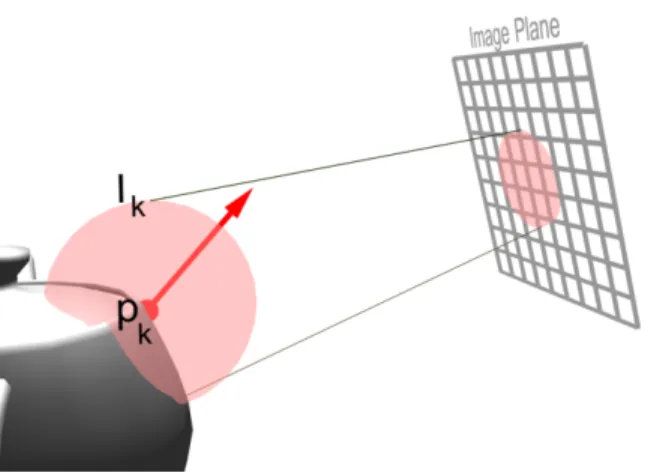
Given a camera, the irradiance splatting splats the sphere Ik onto the image plane (Fig-ure 8.1).
In practice, this splatting is implemented within a vertex shader, where the record properties are stored in the attributes of each vertex of a quadrilateral (−1,−1), (1,−1), (1,1), (−1,1). Note that, while splatting a single point on the screen is also feasible, graphics hardware have a limited maximum point size in pixels, which may complicate the splatting of records with a large zone of influence.
The vertex attributes contain all the fields contained in the record: the position, the surface normal, the harmonic mean distance to the surrounding environment, the irradiance value and the translation/rotation gradients. For the sake of efficiency, the inverse squared harmonic mean is also passed in a vertex attribute.
The weighting function (Equation 8.2) is evaluated for each point visible through pixels covered byIk. Then, the weight is checked against the accuracy value (Equation 8.3). For each
Algorithm 2Pseudo-code for irradiance splatting: Vertex Shader uniform float a;
attribute vec4 recordPosition; attribute vec4 recordNormal; attribute vec3 irradiance; attribute vec3 rotGradR; attribute vec3 rotGradG; attribute vec3 rotGradB; attribute vec3 posGradR; attribute vec3 posGradG; attribute vec3 posGradB; attribute float harmonicMean; attribute float sqInvHarmonicMean;
// Compute the record position in camera space
vec4 camSpacePosition = ModelViewMatrix * recordPosition;
// Compute the splatted sphere of influence in camera space
vec4 splatSphereBox(a*harmonicMean, a*harmonicMean, 0.0, 0.0);
// Compute the actual corners of the box in screen space
vec4 topRight = ProjectionMatrix*( camSpacePosition + splatSphereBox); topRight /= topRight.w;
vec4 bottomLeft = ProjectionMatrix*( camSpacePosition - splatSphereBox); bottomLeft /= bottomLeft.w;
// Deduce the projected vertex position
vec2 delta = topRight.xy - bottomLeft.xy; outputVertex = vec4(
bottomLeft.x + inputVertex.x*delta.x, bottomLeft.y + inputVertex.y*delta.y, 0.0
1.0);
Algorithm 3Pseudo-code for irradiance splatting: Fragment Shader
// Texture containing hit positions
uniform sampler2D hitPositions;
// Texture containing hit normals
uniform sampler2D hitNormals;
// Texture containing hit diffuse
uniform sampler2D hitColors;
// Target accuracy
uniform float a;
// Squared target accuracy
uniform float squaredA;
// Determine the texture coordinate for fetching scene // information from the textures
vec2 textureCoord = vec2(pixelCoord.x,pixelCoord.y);
// Retrieve the corresponding hit position and surface normal
vec3 hitPos = texture2D(hitpos, textureCoord).xyz; vec3 hitNormal = texture2D(hitnorm, textureCoord).xyz;
// Calculate the vector between the hit position and the record
vec3 diff = hitPos-position;
// Estimate the weighting function // Distance factor
float sqrDistance = dot(diff, diff);
float e1 = sqrDistance * sqInvHarmonicMean;
// Normal divergence factor
float e2 = 0.2 * (1.0 - dot(normal , hitNormal));
// First rejection test
if(( e1+e2>squaredA )) discard;
// Evaluate the inverse of the weighting function
float invWeight = (sqrt(e1) + sqrt(e2));
// As the weighting function is infinite at the record // location, perform clamping on the inverse weight
invWeight = max(EPSILON, invWeight);
// Test the final weight against a
if (a<invWeight ) discard;
// From this point, the record is known as usable for // interpolation at the pixel position
Figure 8.1: The sphere Ik around the position pk of the record k is splatted onto the image plane. For each point within the sphere splat, the contribution of recordk is accumulated into the irradiance splat buffer.
pixel passing this test, the algorithm computes the contribution of record k to the outgoing radiance estimate( Algorithm 3).
The outgoing radiance contribution Lo at a point pas seen through a pixel is obtained by evaluating the rendering equation:
Lo(p, ωo) =
Z
H
Li(p, ωi)f(ωo, ωi) cos(θi)dωi (8.5)
whereωiandωoare respectively the incoming and outgoing directions. Li(p, ωi) is the radiance incoming atpfrom directionωi. f(ωo, ωi) is the surface BRDF evaluated for the directionsωi andωo. In the case of irradiance caching, we only consider diffuse interreflections. Therefore, Equation 8.5 simplifies to:
Lo(p) =ρd
Z
H
Li(p, ωi) cos(θi)dωi=ρdE(p) (8.6)
whereρd is the diffuse surface reflectance, andE(p) is the irradiance at pointp. Therefore, the contribution of recordkto the outgoing radiance at pointpis
Lo=ρdEk0(p) (8.7)
where Ek0(p) is the irradiance estimate of record k at point p, obtained through the use of irradiance gradients [WH92, KGBP05].
Note that this splatting approach can be used with any weighting function containing a distance criterion. In this chapter we focused on the weighting function defined in [WRC88], although the function proposed in [TL04] could be employed as well.
8.2
Reducing the Record Count in Interactive
Applica-tions
When computing an irradiance cache in the context of interactive or realtime applications, the number of records must be kept as low as possible to reduce the computation time. However, when a low number of records are used to render an image, circle-shaped artifacts appear at
Algorithm 4Pseudo-code for computing irradiance contribution
// Compute the actual weight
float weight = 1.0 / invWeight;
// Fetch the diffuse reflectance
vec3 hitColor = texture2D(hitColors, textureCoord).xyz;
// Compute the position gradient component
vec3 diffDotPosGradient = vec3( dot(diff, posGradientRed), dot(diff, posGradientGreen), dot(diff, posGradientBlue) );
// Compute the rotation gradient component
vec3 normalsCrossProduct = cross(normal, hitNormal); vec3 nCrossNiDotRotGradient = vec3(
dot(normalsCrossProduct, rotGradientRed), dot(normalsCrossProduct, rotGradientGreen), dot(normalsCrossProduct, rotGradientBlue) ); FragmentColor.rgb = weight*(hitColor.xyz/π)*( irradiance + diffDotPosGradient + nCrossNiDotRotGradient ); FragmentColor.a = weight;
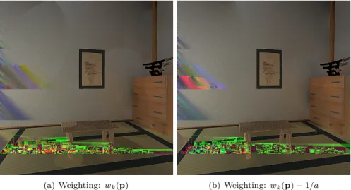
the edge of the zone of influence of the records. This is due to Equation 8.3, in which the contribution of a record is considered null if thew(P)<1/a. The contribution is then abruptly cut at the edge of the zone of influence of the records, yielding the circles. This issue can be simply addressed by subtracting 1/a to the original weighting function proposed in [WRC88]. The record contribution now decreases to 0, yielding a smooth transition with the zones of influence of nearby records (Figure 8.2). Furthermore, the visual impact of potential errors due to over/underestimation of gradients can also be reduced.
8.3
Cache Miss Detection
The rendering process of irradiance caching requires the generation of a number of irradiance records to obtain a reasonable estimate of the indirect lighting for each point visible from the camera. Therefore, even though the values of the records are view-independent, their locations are determined according to the current viewpoint.
Usually, the irradiance cache records are stored in an octree for fast lookups. For a given pixel of the image, a ray is traced in the scene to find the point p visible through this pixel. At this point, the octree is queried to determine whether a new record is required. If yes, the actual indirect lighting is computed atp: a record is created and stored in the cache. Otherwise the cache is used to compute a satisfying estimate if the indirect lighting using interpolation. Since each visible point is processed only once, a newly created record cannot contribute to the indirect lighting of points for which the indirect lighting has already been computed or estimated. Therefore, unless an appropriate image traversal algorithm is employed, artifacts may be visible (Figure 8.3(a)). The traversal typically relies on hierarchical subdivision of the image to reduce and spread the errors. Artifact-free images can only be obtained in two passes: in the first pass,
(a) Weighting: wk(p) (b) Weighting: wk(p)−1/a
Figure 8.2: Indirect lighting computed using 89 irradiance records (a= 0.8) using the original and the new weighting function.
the records required for the current viewpoint are generated. In the second pass, the scene is rendered using the contents of the cache.
On the contrary, the irradiance splatting algorithm is based on the independent splatting of the records. The contribution of a record is splatted onto each visible point within its zone of influence, even though the points have been previously checked for cache miss (Figure 8.3(b)). Therefore, this method avoids the need of a particular image traversal algorithm without harming the rendering quality. For the sake of efficiency and memory coherence, a linear traversal of the image is recommended. Note that, however, any other image traversal algorithm could be used. Once the algorithm has determined where a new record has to be generated, the irradiance value and gradients must be computed by sampling the hemisphere above the new record posi-tion. The following section details a simple method for hemispherical sampling using graphics hardware in the context of 1-bounce global illumination computation.
8.4
GPU-Based Hemisphere Sampling
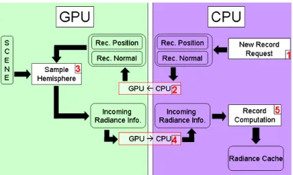
In the method described hereafter, the incoming irradiance associated with a record is generated using both the GPU and CPU. First, the GPU performs the actual hemisphere sampling. Then, the CPU computes the corresponding irradiance value.
8.4.1
Hemisphere Sampling on the GPU
In the context of global illumination, the visibility tests are generally the bottleneck of the algo-rithms. We propose to leverage the power of graphics hardware to speed up the computation. In the classical hemi-cube method [CG85], 5 rendering passes are necessary for full hemisphere sampling. For the sake of efficiency, we preferred a 1-pass method similar to [SP89, LC04]: using a virtual camera placed at the record location, the rasterization engine samples the hemisphere above the record to compute the radiances incoming from each direction. However, as shown in Figure 8.4, using a single rasterization plane cannot account for the radiances incoming from grazing angles. To compensate for the incomplete hemisphere coverage, Larsenet al. [LC04] divide the obtained irradiance by the plane coverage ratio. A more accurate method consists in virtually stretching border pixels to fill the remaining solid angle (Figure 8.4). This method
(a) Octree-based 1 pass (b) Octree-based 2-pass/Splatting 1-pass
Figure 8.3: Upper row: the irradiance records 1, 2, 3, 4 and their respective zones of influence. We consider the use of a sequential traversal of the image for determining the pixels for which a new record is needed. In the classical, octree-based method, a newly created record cannot contribute to pixels which have already been examined. Therefore, discontinuities appear in the contribution zone of the records, yielding artifacts. Those artifacts are illustrated in the upper row: record 1 is created at the point visible through the first pixel, and used for estimating the indirect lighting in the next 3 pixels. When record 2 is created at the point visible through the fifth pixel, its contribution is not propagated to the previous pixels, hence creating a discontinuity. A second rendering pass is needed to generate an image without such discontinuities. Using the irradiance splatting method, each record contributes to all possible pixels, avoiding the need of a second rendering pass. Lower row: the indirect lighting obtained using these methods.
generally yields more accurate results than the approach of Larsenet al. (Table 8.1). Further-more, a key aspect of this method is that the directional information of the incoming radiance remains plausible. Therefore, unlike in [LC04], the indirect glossy lighting could also be rendered correctly if radiance caching is used. A typical aperture size of the virtual camera is twice the aperture of the standard hemicube, that is approximately 126 degrees.
Plane [LC04] Border
sampling stretching
RMS Error 18.1% 10.4% 5.8%
Table 8.1: RMS error of 10000 irradiance values computed in the Sibenik Cathedral scene (Fig-ure 8.9). The border stretching method yields more accurate results than previous approaches, while preserving the directional information of the incoming radiance. The reference values are computed by full hemisphere sampling using Monte Carlo integration.
The GPU-based hemisphere sampling requires a proper shading of the visible points, account-ing for direct lightaccount-ing and shadowaccount-ing. This computation is also carried out by the graphics hard-ware using per-pixel shading and shadow mapping. We recommend using uniform shadow maps
[Wil78]: unlike perspective shadow maps [SD02] or shadow volumes [Hei91], uniform shadow maps are view-independent: in static scenes the shadow map is computed once and reused for rendering the scene from each viewpoint. Therefore, the algorithm reuses the same shadow map to compute all the records, hence reducing the shading cost. Furthermore, the incoming radiances undergo a summation to compute the irradiance. This summation is equivalent to a low-pass filter which blurs out the aliasing artifacts of the shadow maps, hence providing inexpensive, high quality irradiance values.
Once the hemisphere has been sampled, the algorithm computes the actual irradiance record.
Figure 8.4: The hemisphere sampling is reduced to the rasterization of the scene geometry onto a single sampling plane. Since this plane does not cover the whole hemisphere, we use a border compensation method to account for the missing directions. Border pixels are virtually stretched to avoid zero lighting coming from grazing angles, yielding more plausible results.
8.4.2
Irradiance Computation
Figure 8.5: New record computation process. The numbers show the order in which the tasks are processed.
As shown in [LC04] the irradiance is defined as a weighted sum of the pixels of the sampling plane. This sum can be calculated either using the GPU and automatic mipmap generation [LC04], or using frame buffer readback and CPU-based summation (Figure 8.5). In the case of irradiance caching, a record contains the irradiance, the rotational and translational gradients, and the harmonic mean distance to the objects visible from the record location. Such values can typically stored within 22 floating-point values. Hence the method proposed by Larsen
Figure 8.6: The irradiance splatting requires per-pixel information about geometry and materials: the hit point, local coordinate frame, and BRDF.
textures. Even with the latest graphics hardware, this solution turns out to be slower than a readback and CPU-based summation. Furthermore, using a PCI-Express-based graphics card and the asynchronous readbacks provided by OpenGL Pixel Buffer Objects, the pipeline stalls introduced by the readback tend to be very small. However, due to the fast evolution of graphics hardware, the possibility of using GPU-based summation should not be neglected when starting an implementation.
8.5
Global Illumination Rendering
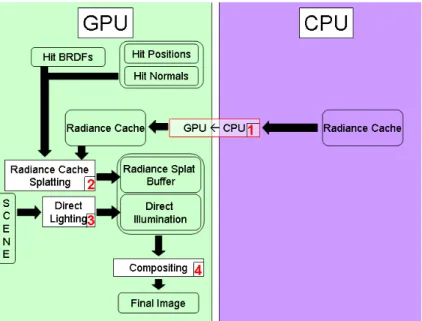
The final image is generated in five main steps (Algorithm 5). Given a camera, the first step consists in obtaining per-pixel information about viewed objects: their position, local coordinate frame and BRDF (Figure 8.6).
In the second and third steps, the rendering process determines where new irradiance records are necessary to achieve the user-defined accuracy of indirect illumination computation. In Step 2, each existing record (possibly computed for previous frames) is splatted onto the splat buffer. Step 3 consists in reading back the irradiance splat buffer into the CPU memory. In Step 4, the algorithm traverses the irradiance splat buffer to determine where new irradiance records are required to achieve the user-defined accuracy (Cache miss detection). For each pixel (x, y) in the irradiance splat buffer, the cumulated weight is checked against the accuracy valuea:
SP LAT BU F F(x, y).w≥a (8.8) If a pixel (x, y) fails this test, the existing cache records are insufficient to achieve the required accuracy. Therefore, a new record is generated at the location visible from pixel (x, y), and is splatted by the CPU onto the irradiance splat buffer (Figure 8.7).
Once SP LAT BU F F(x, y).w≥a for every pixel, the data stored in the cache can be used to display the indirect illumination according to the accuracy constraint. At that time in the algorithm, the irradiance cache stored on the CPU memory differs from the cache stored on the GPU: the copy on the GPU represents the cache before the addition of the records described above, while the copy on the CPU is up-to-date.
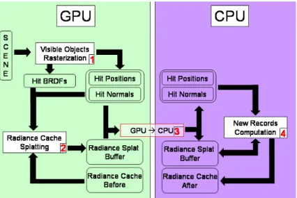
The last rendering step is the generation of the final image using the cache contents (Fig-ure 8.8). The irradiance cache on the GPU is updated, then the irradiance splatting algorithm is applied on each newly generated cache record. Hence the irradiance splat buffer contains the cumulated record weight and outgoing radiance contribution of all the irradiance records. Then,
Algorithm 5Global illumination rendering //Step 1
Generate geometric and reflectance data of objects viewed through pixels (GPU) Clear the splat buffer
//Step 2
for allcache recordsdo
//The irradiance cache is empty for the first image,
//and non empty for subsequent images
Algorithm 1: splat the records onto the irradiance splat buffer (GPU)
end for
//Step 3
Read back the irradiance splat buffer from GPU to CPU //Step 4
for allpixels (x, y) in the irradiance splat bufferdo if SP LAT BU F F(x, y).w < athen
Compute a new incoming radiance record at corresponding hit point (GPU/CPU) Apply Algorithm 1: splat the new record (CPU)
end if end for
//Step 5
for allcache recordsdo
Apply Algorithm 1: splat all the newly generated records (GPU)
end for
//Normalize the irradiance splat buffer (GPU)
for allpixels (x, y) in the irradiance splat bufferdo
SP LAT BU F F(x, y).Lo/=SP LAT BU F F(x, y).w
end for
Combine the irradiance splat buffer with direct lighting (GPU)
Figure 8.7: The irradiance cache filling process. The numbers show the steps defined in Algorithm 5. During this process, the irradiance cache stored on the CPU is updated whereas the copy on the GPU remains untouched.
Figure 8.8: The final rendering task. The numbers show the processing order described in steps 4 and 5 of Algorithm 5.
the cumulated contribution at each pixel is divided by cumulated weight. This process yields an image of the indirect lighting in the scene from the current point of view. Combined with direct lighting, this fast method generates a high quality global illumination solution.
8.6
Implementation Details
This section gives technical information about the implementation of irradiance splatting. The rendering algorithm is based on deferred shading: the information on visible points is generated in a first pass by rasterizing the scene geometry. This information is used as the input of the irradiance splatting. Using this method, the most costly operations are only performed once for each pixel of the final image.
As shown in Figures 8.7 and 8.8, this rendering algorithm makes intensive use of the GPU computational power. The required base information (Figure 8.6) is generated by rasterizing the scene geometry on the GPU using a dedicated shader. Using multiple render targets, this shader renders all the necessary information in a single rendering pass. Figure 8.6 shows that this step includes the storage of per-pixel BRDF. In the case of irradiance caching, this information is the diffuse reflectance of the material (i.e. one RGB value). During splatting, the reflectance is combined with the irradiance contributions of the records.
The irradiance splatting can be performed either using the GPU or the CPU. Both are necessary, depending on the current context as explained hereafter. The irradiance splatting on the GPU is performed by drawing a quadrilateral and a dedicated vertex shader described above. Then, the splatting fragment shader processes each fragment so that its value represents the weighted contribution of the record. The fragment is accumulated in the irradiance splat buffer using the floating-point blending capabilities provided by graphics hardware. The final normalization (i.e. the division by the cumulated weight) is performed using a fragment shader in an additional pass for the final display.
The cache miss detection is performed by traversing the irradiance splat buffer sequentially using the CPU. Consequently, the GPU-based splatting cannot be used efficiently during the record addition step: this would require to read back the irradiance splat buffer from the GPU
memory after the computation and splatting of each new record. The CPU implementation is designed the same way as for the GPU. Figure 8.6 shows that the irradiance splatting requires information about the visible objects. This information is computed on the GPU, then read back to the main memory once per frame. The overhead introduced by the data transfer from GPU to CPU turns out to be very small using PCI-Express hardware.
Once all necessary records are computed and splatted onto the irradiance splat buffer, the final picture containing both direct and indirect lighting has to be generated. The direct lighting computation is straightforwardly carried out by the GPU, typically using per-pixel lighting and shadow maps [Wil78, BP04]. To reduce the aliasing of shadow maps without harming the performance, we use high definition shadow maps (typically 1024×1024) with percentage-closer filtering [RSC87] using 16 samples. Hence the same shadow map can be used for both the record computation and the rendering of direct lighting in the final image. Note that higher quality images could be obtained using view-dependent shadowing methods such as shadow volumes for the visualization of the direct lighting in the final image.
The normalization of the irradiance splat buffer and the combination with direct lighting are finally performed in a single fragment shader which displays the final image.
8.7
Results
Note: the images and timings have been generated using an nVidia Quadro FX 3400 PCI-E and a 3.6 GHz Pentium 4 CPU with 1 GB RAM.
8.7.1
High Quality Rendering
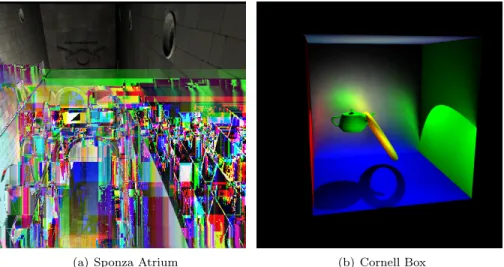
This section details non-interactive high quality global illumination computation. First, we com-pare the results obtained with our GPU-based renderer with the well-known Radiance software [War94] in the context of irradiance caching.
We have compared the rendering speed of the Radiance software and our renderer in diffuse environments: the Sibenik Cathedral and the Sponza Atrium (Figure 8.10). The images are rendered at a resolution of 1000×1000 and use a 64×64 resolution for hemisphere rasterization. The results are discussed hereafter, and summarized in Table 8.2.
a) Sibenik Cathedral This scene contains 80K triangles, and is lit by two light sources. The image is rendered with an accuracy parameter of 0.15. At the end of the rendering process, the irradiance cache contains 4076 irradiance records. The irradiance splatting on the GPU is performed in 188 ms. The Radiance software rendered this scene in 7 min 5 s while our renderer took 14.3 s, yielding a speedup of about 30×.
b) Sponza Atrium This scene contains 66K triangles and two light sources. Using an accuracy of 0.1, this image is generated in 13.71 s using 4123 irradiance records. These records are splatted on the GPU in 242.5 ms. Using the Radiance software with the same parameters, a comparable image is obtained in 10 min 45 s. In this scene, our renderer proves about 47×faster than the Radiance software.
8.7.2
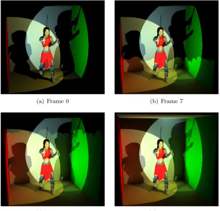
Interactive Global Illumination
An important aspect of the irradiance caching algorithm is that the values of the records are view-independent. In a static scene, records computed for a given viewpoint can be reused for other camera positions. Therefore, the irradiance splatting approach can also be used in the context of interactive computation of global illumination using progressive rendering. The direct lighting being computed independently, the user can walk through the environment while the irradiance cache is filled on the fly. Figure 8.11 shows sequential images of Sam scene
(a) Radiance (b) Our renderer
Figure 8.9: The Sibenik Cathedral scene (80K triangles). The images show first bounce global illumination computed with Radiance (a) and our renderer (b) (Model courtesy of Marko Dabrovic)
(a) Sponza Atrium (b) Cornell Box
Figure 8.10: Images obtained with our renderer. The Sponza Atrium (66K triangles) is only made of diffuse surfaces (Model courtesy of Marko Dabrovic). The Cornell Box (1K triangles) contains a glossy back wall.
Sibenik Cathedral Sponza Atrium
Triangles 80K 66K
Accuracy 0.15 0.1
Radiance time (s) 425 645
Our renderer time (s) 14.3 13.7
Speedup 29.7 47.1
Table 8.2: Rendering times obtained using Radiance and irradiance splatting for high quality rendering of diffuse environments. Each image is rendered at resolution 1000×1000.
(63K triangles) obtained during an interactive session with an accuracy parameter of 0.5 and resolution 512×512. The global illumination is computed progressively, by adding at most 100 new records per frame. Our renderer provides an interactive frame rate (between 5 and 32 fps) during this session, allowing the user to move even though the global illumination computation is not completed. This method has been used for interactive walkthroughs in diffuse and glossy environments such as theSibenik Cathedral and theCastle.
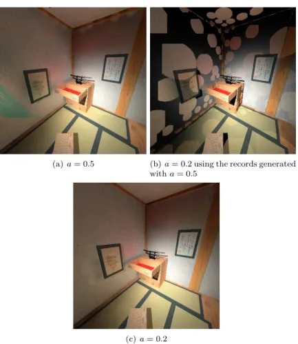
In this context, the irradiance splatting also proves useful for adjusting the value of the user-defined accuracy parametera. In the classical irradiance caching method, the structure of the octree used to store the records is dependent ona. Therefore, the octree has to be regenerated for each new value ofa. Using this approach the size of each splat is computed for each frame on the GPU, hence allowing the user to tune the value ofainteractively to obtain the desired visual quality (Figure 8.12).
(a) Frame 0 (b) Frame 7
(c) Frame 11 (d) Frame 14
Figure 8.11: A progressive rendering session for interactive visualization of theSam scene (63K triangles). Our renderer computes at most 100 new records per frame, hence maintaining an interactive frame rate (5 fps) during the global illumination computation. When the irradiance cache is full, the global illumination solution is displayed at 32 fps.
8.8
Conclusion
This chapter presented a reformulation of the irradiance caching algorithm by introducing irradi-ance splatting. In this method, the sphere of influence of each record is splatted onto the image plane. For each pixel within the splatted sphere, a fragment shader computes the contribution and weight of the record to the indirect lighting of the corresponding point. The record weight
(a)a= 0.5 (b)a= 0.2 using the records generated witha= 0.5
(c)a= 0.2
Figure 8.12: The irradiance splatting method allows for the dynamic modification of the user-defined accuracy valuea, hence easing the parameter tuning process.
and weighted contribution are accumulated into the irradiance splat buffer using floating-point alpha blending. The final indirect lighting of visible points is obtained by dividing the weighted sum of the records by the cumulated weights in a fragment shader. Using this approach, each record contributes to all possible pixels, hence simplifying the cache miss detection algorithm. By avoiding the need of complex data structures and by extensively using the power of graphics hardware, the irradiance splatting allows for displaying global illumination in real-time.
Another speedup factor is the use of both GPU and CPU to compute the values of the irradiance records. While the GPU performs the costly hemisphere sampling, the CPU sums up the incoming radiances to compute the actual values and gradients of the records. This method requires many data transfers from the GPU to the CPU. Even though classical architectures such as AGP [Int02] would have introduced a prohibitive bottleneck [CHH02], the new PCI-Express 16×port [PCI03] provides transfer rates up to 8GB/s. Compared to AGP, the pipeline stalls are drastically reduced, making this method usable even in the case of on-the-fly computation of global illumination for interactive rendering.
[BP04] Michael Bunnell and Fabio Pellacini. GPU Gems: Shadow map antialiasing, pages 185–192. Addison Wesley, 1 edition, 2004.
[CG85] Michael Cohen and Donald P. Greenberg. The Hemi-Cube: A Radiosity Solution for Complex Environments. InProceedings of SIGGRAPH, volume 19, pages 31–40, August 1985.
[CHH02] Nathan A. Carr, Jesse D. Hall, and John C. Hart. The ray engine. InProceedings of the ACM SIGGRAPH/EUROGRAPHICS conference on Graphics hardware, pages 37–46. Eurographics Association, 2002.
[Hei91] Tim Heidmann. Real shadows, real time. Iris Universe, 18:23–31, 1991. [Int02] Intel Corporation. AGP v3.0 Specification. 2002.
[KGBP05] Jaroslav Kˇriv´anek, Pascal Gautron, Kadi Bouatouch, and Sumanta Pattanaik. Im-proved radiance gradient computation. InProceedings of SCCG, pages 149–153, 2005. [LC04] Bent Dalgaard Larsen and Niels Jorgen Christensen. Simulating photon mapping for real-time applications. In A. Keller and H. W. Jensen, editors, Proceedings of Eurographics Symposium on Rendering, pages 123–131, June 2004.
[PCI03] PCI-SIG. PCI-Express v1.0e Specification. 2003.
[RSC87] W.T. Reeves, D.H. Salesin, and R.L. Cook. Rendering antialiased shadows with depth maps. InProceedings of SIGGRAPH, volume 21, pages 283–291, August 1987. [SD02] Marc Stamminger and George Drettakis. Perspective shadow maps. In Proceedings
of SIGGRAPH, July 2002.
[SP89] Francois Sillion and Claude Puech. A General Two-Pass Method Integrating Specular and Diffuse Reflection. InProceedings of SIGGRAPH, volume 23, pages 335–344, July 1989.
[TL04] Eric Tabellion and Arnauld Lamorlette. An approximate global illumination system for computer-generated films. InProceedings of SIGGRAPH, August 2004.
[War94] Gregory J. Ward. The RADIANCE Lighting Simulation and Rendering System. InComputer Graphics Proceedings, Annual Conference Series, 1994 (Proceedings of SIGGRAPH, pages 459–472, 1994.
[WH92] Gregory J. Ward and Paul Heckbert. Irradiance Gradients. InProceedings of Euro-graphics Workshop on Rendering, pages 85–98, Bristol, UK, May 1992.
[Wil78] Lance Williams. Casting curved shadows on curved surfaces. In Proceedings of SIGGRAPH, pages 270–274, 1978.
[WRC88] Gregory J. Ward, Francis M. Rubinstein, and Robert D. Clear. A Ray Tracing Solution for Diffuse Interreflection. InProceedings of SIGGRAPH, volume 22, pages 85–92, August 1988.