Feature extraction using MPEG-CDVS and Deep Learning with application to robotic navigation and image classification

(1)

04 August 2020

POLITECNICO DI TORINO

Repository ISTITUZIONALE

Feature extraction using MPEG-CDVS and Deep Learning with application to robotic navigation and image classification / PORTO BUARQUE DE GUSMAO, Pedro. - (2017).

Original

Feature extraction using MPEG-CDVS and Deep Learning with application to robotic navigation and image classification

Publisher:

Published

DOI:10.6092/polito/porto/2665943 Terms of use:

Altro tipo di accesso

Publisher copyright

(Article begins on next page)

This article is made available under terms and conditions as specified in the corresponding bibliographic description in the repository

Availability:

This version is available at: 11583/2665943 since: 2017-02-23T23:32:22Z Politecnico di Torino

(2)

Doctoral Program in Electronic and Communications Engineering (28thcycle)

Feature Extraction Using

MPEG-CDVS and Deep Learning

with Application to Robotic

Navigation and Image Classification

By

Pedro Porto Buarque de Gusmão

******

Supervisor(s):

Prof. Enrico Magli

Doctoral Examination Committee:

Prof. Carla Fabiana Chiasserini, Politecnico di Torino Prof. Matteo Cesana, Politecnico di Milano

Prof. Sergio Saponara, Università degli Studi di Pisa Politecnico di Torino

(3)

Declaration

I hereby declare that, the contents and organization of this dissertation constitute my own original work and does not compromise in any way the rights of third parties, including those relating to the security of personal data.

Pedro Porto Buarque de Gusmão 2017

* This dissertation is presented in partial fulfillment of the requirements forPh.D. degreein the Graduate School of Politecnico di Torino (ScuDo).

(4)

(5)

Acknowledgements

The research presented in this thesis has been supported by TIM, former Telecom Italia. Besides thanking my supervisor Prof. Enrico Magli, I would also like to thank my colleagues at the TIM Visible Lab, Skjalg Lepsøy, Gianluca Francini and Massimo Balestri for all the help they provided me and all the good times we have shared. I must also thank my good friend Stefano Rosa for the help he gave me regarding the mechanical aspects of robotics and for the insightful discussions shared with a cup of coffee.

Finally, this work would not have been possible without the support received from my friends, my family and from my girlfriend, Elisabetta Bichiri.

(6)

The main contributions of this thesis are the evaluation of MPEG Compact Descriptor for Visual Search in the context of indoor robotic navigation and the introduction of a new method for training Convolutional Neural Networks with applications to object classification.

The choice for image descriptor in a visual navigation system is not straightfor-ward. Visual descriptors must be distinctive enough to allow for correct localization while still offering low matching complexity and short descriptor size for real-time applications. MPEG Compact Descriptor for Visual Search is a low complexity image descriptor that offers several levels of compromises between descriptor dis-tinctiveness and size. In this work, we describe how these trade-offs can be used for efficient loop-detection in a typical indoor environment. We first describe a probabilistic approach to loop detection based on the standard’s suggested similarity metric. We then evaluate the performance of CDVS compression modes in terms of matching speed, feature extraction, and storage requirements and compare them with the state of the art SIFT descriptor for five different types of indoor floors.

During the second part of this thesis we focus on the new paradigm to machine learning and computer vision called Deep Learning. Under this paradigm visual fea-tures are no longer extracted using fine-grained, highly engineered feature extractor, but rather using a Convolutional Neural Networks (CNN) that extracts hierarchical features learned directly from data at the cost of long training periods.

In this context, we propose a method for speeding up the training of Convolutional Neural Networks (CNN) by exploiting the spatial scaling property of convolutions. This is done by first training apre-trainCNN of smaller kernel resolutions for a few epochs, followed by properly rescaling its kernels to thetarget’s original dimensions and continuing training at full resolution. We show that the overall training time of a

(7)

vi

convolutions during early stages of learning. Moreover, by rescaling the kernels at different epochs, we identify a trade-off between total training time and maximum obtainable accuracy. Finally, we propose a method for choosing when to rescale kernels and evaluate our approach on recent architectures showing savings in training times of nearly 20% while test set accuracy is preserved.

(8)

List of Figures

2.1 Modern representation of SLAM problem. . . 4 2.2 Pinhole camera model. . . 6 3.1 SIFT detection: Keypoints are defined as extrema in the scale-space

difference-of-Gaussian function both locally and in scale. . . 14 3.2 SIFT descriptor generation: A 16x16 pixel grid is center at the

detected keypoint. For each 4x4 subregion the descriptor generates an 8-bin orientation histograms. . . 15 3.3 MPEG Compact Descriptor for Visual Search pipeline. . . 17 4.1 The first row corresponds to original classic approach to object

detection. The second row represents classic approach to object classification. Bottom row represent the Deep Learning approach where each feature level is learned. . . 25 4.2 Usual representation of a feedforward neural network and its

associ-ated artificial neuron model. . . 26 4.3 Basic structure of a Convolutional Neural Network. A number of

aternating convolutional and pooling layers is applied to the input for feature extraction followed by a sequence of one or more fully-connected layers. . . 27 4.4 Convolutional Layer: Each kernel performs channel-wise 2D

convo-lutions to produce a single channel in the output set of feature-map. 28 4.5 Commonly used activation functions. . . 29

(13)

xii List of Figures

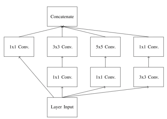
4.6 Inception module. . . 32

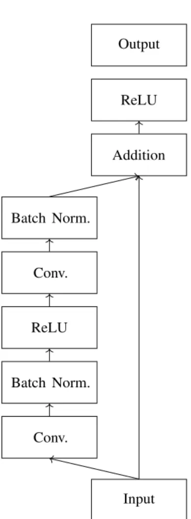
4.7 Residual block architecture. . . 33

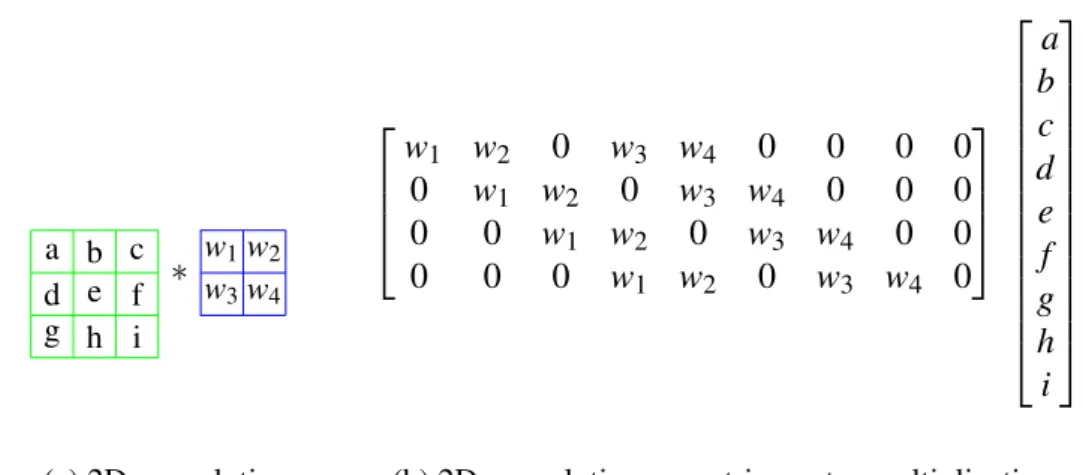
5.1 2D convolution using matrix-vector multiplication. The concept can be extended for multi-channels inputs and kernels using concatenation. 39 6.1 Robot viewpoint and relative coordinate frame. . . 48

6.3 ROS Nodes for MPEG-CDVS Visual SLAM system. . . 50

6.4 Different types of floorings commonly found in indoor environments. Names were assigned according to the flooring’s visible attributes. . 51

6.5 Average number of extracted local descriptors per image for each type of flooring. . . 52

6.6 Visual representation oflocal scorefor different flooring types. . . . 55

6.7 Visual representation oflocal scorefor the Printed Wood floor using different compression modes. . . 56

6.8 Visual representation of SIFT for different floor types . . . 57

6.9 Cumulative loop probability for printed wood floor. . . 59

6.10 Path comparison using visual odometry. . . 61

6.11 Paths optimized using LAGO. . . 63

6.12 Map and path generated with a laser scanner and Gmapping algorithm. 66 7.1 Training starts with apre-trainnetwork of smaller convolution ker-nels and input images. After a number of epochs, kerker-nels are resized to thetarget’s resolution and training continues as scheduled. . . 68

7.2 Visual representation of the interface between convolutional and fully-connected layers. Feature-maps from a convolutional layer are first vectorized before entering a fully-connected layer, whose weights are usually represented in matrix form. The number of input must be selected according to the new feature-map spatial resolution ( ˜W,_H˜_{) and the number of output neurons}_n_out _{is kept invariant. . . .} ₇₂

(14)

7.3 Rescaling weights in fully-connected layer back totarget’s dimen-sions. Each column in the fully-connected weight matrix is reshaped to match thepre-trainfeature-map dimensions. Rescaling is applied in the same fashion as regular convolutional kernels and weights are then vectorized to thetarget’s new weight matrix. . . 73 7.4 Accuracy as function of epochs obtained using both original

OverFeat-fastof input resolution 231_×231 and itspre-traincounterpart having 147_×147 input resolution. . . 76 7.5 Accuracy as function time obtained using both original OverFeat-fast

of input resolution 231_×231 and itspre-train counterpart having 147_×147 input resolution. . . 77 7.6 Effects of rescaling kernels at different epochs. Lower and upper

horizontal lines define the maximum accuracies obtained with pre-trainandtargetnetworks, respectively. . . 78 7.7 Accuracy as a function of epochs when training is allowed to

con-tinue using current learning rules for a few extra epochs. Learning rule is updated as soon as there is a drop in test accuracy. . . 80 7.8 Accuracy as a function of time when training is allowed to continue

using current learning rules for a few extra epochs. Learning rule is updated as soon as there is a drop in test accuracy. . . 81 7.9 Accuracy curves obtained using ResNet-34 as a function of epochs.

Lower and upper horizontal lines define the best accuracies obtained for the new baseline networks. . . 82 7.10 Accuracy curves obtained using ResNet-34 as a function of time.

Lower and upper horizontal lines define the best accuracies obtained for the new baseline networks. . . 82

(15)

List of Tables

3.1 Maximum descriptor length in bytes for each mode of compression. 18 3.2 Number of selected transformed dimensions used by each mode of

compression. . . 19 6.1 Average extraction times per image in milliseconds for each CDVS

mode of compression and SIFT. . . 53 6.2 Average matching times per image in milliseconds for each CDVS

mode of compression and SIFT. . . 54 6.3 Hypothesized values for local score loop detection. . . 59 6.4 Experiemtal threshold values for local score loop detection. . . 62 6.5 Relative pose errors between starting and final position for both

visual odometry and VSLAM. . . 64 6.6 Storage requirement for all 7154 images and total matching time

between last sequence image and all previous ones. . . 64 7.1 Suggested kernel resolution conversions with relative resize factors

and bounds. . . 70 7.2 Architecture description of Pre-train network based on Overfeat-fast.

Values in bold indicate differences with respect to original model. . 75 7.3 Effect of resizing kernels on storage requirements, accuracy and

(16)

7.4 Final accuracy and training times for resized networks after a total of 55 epochs. Lower and upper bound accuracies are set bypre-train

andtargetnetworks, respectively. . . 79 7.5 Best accuracy and total training times for resized networks with extra

training. . . 80 7.6 Best accuracy and training times for ResNet-34. Training is reduced

by 33.7 hours when upscaling two epochs before changing learning rate. . . 83

(17)

Chapter 1

Introduction

Visual features play a fundamental role in all computer vision tasks. They are intended to encode fundamental aspects in an image that are useful for solving specific problems such as face recognition, object classification, robotic localization, etc. Each of these tasks comes with a set of requirements such as response time constraints, accuracy and limited computational resources. Very often a compromise between those three must be attained, which is reflected in the choice of visual feature being used. It is also true, however, that some of these tasks share similar underlying requirements and visual features used for solving one problem could also be used for solving the other. Such similarity can be found between the tasks of large scale object recognition and robotic visual localization, and it is one of the subjects of this thesis.

In robotic navigation, an indoor robot that navigates throughout an environment using images from camera for orientation must compare what it is currently viewing with previously seen landmarks in order to estimate its motion and current position. Such landmarks, commonly referred to as visual features, must be distinctive and of fast comparison for reliable localization and motion estimation. In a seemingly different application, systems that perform image search over based on visual content, known as Content-Based Image Retrieval (CBIR) systems, must also compare a query image of an object against a database and return only the ones that effectively contain the object. Besides being accurate, CBIR response time must also be short not sacrifice the so called user-experience.

(18)

The similarity between requirements in these two problems suggests the use of similar solutions. Very recently, the Moving Picture Experts Group (MPEG) has defined a new industry standard for CBIR known as Compact Descriptors for Visual Search (MPEG CDVS) [1]. The standard specifies various modes of compression that offer trade-offs between descriptor distinctiveness and size and also suggests specific metrics to quantify similarity between images. The first part of this thesis is concerned with the use of this new visual descriptor on the context of robotic navigation.

On the one hand, if it is true that similar tasks may share similar solutions, on the other hand, problems that look similar at first might as well have very differ-ent requiremdiffer-ents. This is the case for the tasks of object recognition and object classification. The former requires the identification of one specific object such as “Mole Antonelliana", while the latter must be able to encode the broader semantic definitions such as “landmark". The difficulty in solving the latter problem lies in fact class “landmark" represents a semantic definition, which encodes countless variations in visual aspects, while the “Mole Antonelliana" is, to some extent, unique.

For many years, however, these two problems were approached using the same visual features which has led to very limited performances in classification tasks. Fortunately enough, in the past few years, the field of computer vision has witnessed a shift of paradigm called Deep Learning, where visual features are no longer de-signed by computer vision experts but rather they are learned directly from data. This approach has defined new state-of-the-art in image classification and was made possible due to the recent availability of large training datasets and the use of GPUs for massive parallel computation. However, benefits of learning task-oriented fea-tures from large datasets come at the cost of long training periods of computationally demanding neural networks, that take weeks to produce desirable results. The second part of this thesis is dedicated to the development of a novel training technique de-signed to reduce training times of Convolutional Neural Networks (CNN), a family of networks especially developed to learn features for object classification.

(19)

Chapter 2

Simulataneous Localizantion and

Mapping

In robotic navigation, the problem of generating a representation of the robot’s environment while estimating its relative pose is called Simultaneous Localization and Mapping (SLAM). The difficulty in solving SLAM problems lies in its own formulation: a robot’s pose must be referred to a map, while the details of a map are measured from relative poses. Moreover, in order to perform measurements and navigation, robots rely on physical sensors and actuators which are limited in precision. Given these inherited uncertainties, modern formulations of SLAM define this problem as a probability function of the robot’s pose p_t and map’s attributem

conditioned to a sequence of observationso_1:_t, i.e.P(p_t,m_t_|o_1:_t).

The definition of pose is usually given by a set of coordinates and direction; however, the precise definition of a map’s attributes and observations depend on the particular configuration of environment and sensors being used. When maps are associated to higher-level tasks such as path planning and collision avoidance, it must contain physical information about objects such as position and volume. However, the ultimate use of a map is to provide spatial reference to the robot, so that map attributes require precise positioning and unique identifiers. The observations, on the other hand, are a collection of signals obtained from sensors and signals applied to actuators. Signals applied to an actuator usually have a direct meaning in SLAM, such as "move forward 10 cm". On the other hand, information coming from sensors such as cameras and laser-scanner, must first be analyzed and associated to elements

(20)

in the environment, in a process calleddata association, so that it can be useful for estimating pose and the map’s attributes.

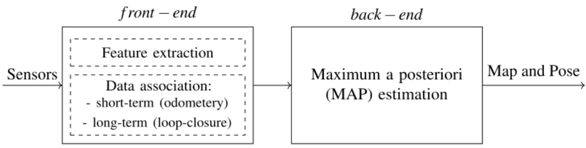
This current formulation of the SLAM problem is summarized in Figure 2.1 adapted from [2], which divides the SLAM problem into two blocks. Thefront-end

is responsible for acquiring data and using it for motion estimation (odometry) and place recognition (loop-detection), while the second block is responsible for generat-ing an optimized representation of the map and robot’s path given all observations. This work is mainly concerned withfront-end block of SLAM that uses a single camera as sensor to produce odometry and loop-closure from visual features. We shall describe these components with detail and briefly describe the back-end. For an extensive and up-to-date overview of SLAM, the interested reader is referred to [2].

f ront₋end Sensors Feature extraction Data association: - short-term (odometery) - long-term (loop-closure) Maximum a posteriori (MAP) estimation back₋end

Map and Pose

Fig. 2.1 Modern representation of SLAM problem.

2.1

Visual Odometry

Visual Odometry (VO) is the process of estimating a robot’s egomotion, i.e. its displacement relative to a static scene, using information provided by one or more cameras attached to it. The term was first used by Srinivasanet al.in [3] and derives from wheel encoder odometry, a process commonly used by ground vehicles which counts the number of revolutions a wheel performs in order to estimate a cumulative displacement. Visual Odometry infers motion from sequences of images, which makes it insensitive to wheel drifting, although it does require the environment to have sufficient visual texture and illumination.

(21)

2.1 Visual Odometry 5

Monocular and Stereo VO

VO can be classified as either monocular or stereo depending on the number of cameras being used and on their particular setup. Stereo VO can directly retrieve the 3D positions of points in the environment through triangularisation, which is usually done using multiple cameras having known relative position [4–8], but can also be achieved using a single sliding camera that registers the scene from different viewpoints each time the robot stops [9]. Monocular VO, on the other hand, estimates motion using just one camera that takes just one picture at each position [10–12]. This approach can only estimate displacements up to a scaling factor. This apparent disadvantage can be overcome when using other sources of information such as measuring known objects in the image, or by including additional sensors like laser-scanner.

Visual features

Methods for estimating motion using monocular VO can be appearance-based, feature-based [13, 12, 14] or even a combination of these two. Appearance-based methods use pixel intensity from the entire image in order to estimate motion, while feature-based methods infer displacements from just a few interest points (also known as keypoints) that appear in consecutive images. The process of choosing which points should be used for motion estimation is called keypoint detection, while the process of finding similar keypoints across a sequence of images is called feature matching. The exact procedures with which features are detected and extracted depend on the feature detector and descriptor being used.

Keypoint detectors generally found in literature can be classified as either blob detectors or corner detectors. A corner is defined as an intersection of edges while a blob is small region in the image that differs from immediate neighbors in all directions in terms of illuminate intensity. Corners are usually faster to extract and better localized spatially; however, blobs are usually more distinctive and better localized in scale.

Important characteristics of a feature detectors in the field of robotics include: good spatial and scale localization, which improves motion estimation; repeatabil-ity, so that the same points are found in consecutive images; robustness to noise, compression artifacts and blur, so that low cost cameras can be used; and of fast

(22)

p f C Y Z f Y / Z y Y x X x p image plane camera centre Z principal axis C X

Fig. 2.2 Pinhole camera model.

detection so that will it not limit the speed of the robot. Desired properties for feature descriptors include: robustness to change in viewpoint and illumination so that should these conditions changes the overall feature vector will remain nearly the same; distinctiveness, so that interest point will not mismatch producing wrongfully associated data; small data footprint so that large maps can be generated using limited hardware; and fast extraction and matching times, again not to impose limits to the robot’s mobility.

In this work, we are primarily concerned with feature-based Monocular Visual Odometry for indoors, planar environment. We shall we describe the process by which features that have already been matched between consecutive frames can be used for motion estimation. A broader overview on Visual Odometry is found in [15, 16].

2.1.1

Camera Model and Calibration

Estimating 3D motion from just a set of matching pixels requires a mapping between 3D world coordinates to 2D image pixel coordinates. The most commonly used method for doing this is by first using the pinhole camera model [17] followed by a change in coordinate systems.

Under the pinhole model, light emitted from 3D points pass through theimage planeand meet at the camera center. Thez₋axis in this camera coordinate system is called theprincipal axis and intersects the image plane perpendicularly at the

principal point. A representation of this model may be seen in Figure 2.2 extracted from [17].

(23)

2.1 Visual Odometry 7

Intrinsic Parameters

The pinhole model makes two strong assumptions that might not always be true. It assumes that the origin of the image plane is at the principal point and that pixels in the camera sensors are squares. The first issue can be corrected by considering an offset of(p_x,p_y), while the second issue can be adapted by considering different values of focal distances αxand αyfor each axis. These parameters are known as

the camera’s intrinsic parameters and are used to transform 3D points from camera’s coordinate points to 2D points in pixel coordinates as seen in (2.1).

s    u v 1   =    αx 0 px 0 αy py 0 0 1       x_cam y_cam z_cam    (2.1) Extrinsic Parameters

Depending on the camera’s position and on the robot’s motion constraints, represent-ing 3D points in the camera’s coordinates might not be the most appropriate choice. In fact, in our work we extract visual features from the floor plane so that points in our setup will have world coordinatez_w=0, which in turn allows us to reduce our problem to a planar homography as described in [18].

s    u v 1   = K[R|T]      x_w y_w z_w 1      (2.2)

However, for general motion models, a rotation matrixR_∈SO(3)and a trans-lation column vectorT _∈_R3are usually needed, which make up for the camera’s extrinsic parameters. The complete transformation is represented in (2.2) withK

being the camera’s intrinsic parameters matrix.

Distortion Coefficients

Finally, due to manufacturing processes, lenses may display distortions that are not modeled by the pinhole camera but which can influence the correct 2D-3D mapping.

(24)

Radial distortion is generated by the curvature of the lens and it causes straight lines in the edges of the images to appear curved. Tangential distortion, on the other hand, occurs when the image plane is not aligned with the lens.

Fortunately, the problem of camera distortion has been throughly investigated [19–21] and many are the software available that are able correctly estimate these parameters from a sequence of patterned images such as chessboards. In this work we have used the computer vision camera calibration toolbox from MATLAB to retrieve the sets of intrinsic and extrinsic parameters along with distortion coefficients.

2.1.2

Motion Model

In our scenario, a robot carrying a fixed camera moves though an unknown en-vironment acquiring a sequence of pictures at discrete times k. For each pair of consecutive imagesI_k₋₁andI_k we perform feature extraction and matching, which results into two sets ofN matching coordinate pairs. Precise description of how matching is performed is postponed until the next chapter. We combine these pixel coordinates with the camera’s intrinsic and extrinsic parameters and produce the sets

P_k₋₁andP_k each containing the 3D coordinates for theNmatching pairs.

By defining Pb_k−₁ and Pb_k to be the centroids of sets P_k−₁ and P_k respectively, we follow the approach for rotation and translation estimation from sets of points described in [22] and apply Singular Vector Decomposition (SVD) on the correlation matrixE. E= N

∑

i=1 (P_ki₋Pbk)(Pki₋1−Pbk₋1)T (2.3) [U,S,V] =SV D(E) (2.4)

Rotation matrix and translation vector between successive frames are then ob-tained as follows:

(25)

2.2 Loop-Closure 9

R_k₋₁_,_k=VUT (2.5)

T_k₋₁_,_k=−(R_k₋₁_,_kPb_k) +Pb_k₋₁ (2.6) The set of all R_k₋₁_,_k and T_k₋₁_,_k are then used as odometry constraints to the SLAM problem.

2.2

Loop-Closure

Loop-closure detection consists in identifying points in the path that have already been visited by the robot. Loop-closure improves visual odometry in two ways: first, pose estimation obtained by simply accumulating odometry inherently accumulates also measurement errors, which in turn makes the approach unreliable over long trajectories. In this sense, correctly identifying previously seen scenario improves the robot’s belief regarding its pose and map attributes. Second, visual odometry by itself is unable to construct globally consistent maps. Since VO only compares features between consecutive frames, it is bound to represent loops as distinct places.

In Visual SLAM, the process of detecting loops is very similar to Visual Odome-try with the exception that features being matched are not extracted from consecutive frames but rather they are compared to a larger pool of features from the robot’s expected vicinity. In the worse case scenario, known as the kidnapped robot, the robot is moved from its position by an external agent and comparison between features must be done with the entire dataset.

Loop detection also produces relative poses represented by a rotation matrix and a translation vector; however, these loop-closure constraints are relative to past poses as inR_k_,_k₋_N andT_k_,_k₋_N.

2.3

Maximum a Posteriori Optimization

Algorithmic approaches to solve the optimization part of the SLAM problem are usu-ally divided into three classes: particle-filtering [23], Gaussian filter-based methods [24], and graphical approaches [25–28]. In this work we chose to use a graphical

(26)

approach to SLAM known as Linear Approximation for Pose Graph Optimization (LAGO) [28].

LAGO solves the SLAM optimization problem by allowing relative observations obtained from visual odometry and loop-closure to define a graphs of constraints. In this graph, poses are defined as nodes, while relative motion between poses are represented by the graph’s edges. LAGO assumes that observations are independent and affected by zero-mean Gaussian noise for both rotation and translation.

(27)

Chapter 3

Visual Feature Descriptors

In the previous chapter we have seen how visual features play an important role in Visual SLAM for both motion estimation and loop detection. As a matter of fact, visual features were first used to solve visual navigation [9] and the closely related problem of structure from motion (SfM) [29, 30], i.e. to reconstruct a 3D scene and camera trajectory from a sequence of images.

The problem of recognizing specific objects in a scene came later and became known in computer vision as object recognition. Early attempts to solve this problem would first model the query object using 3D primitives such lines, ellipses and vertex and then try to match those primitives to the candidate image [31, 32]. A second approach, which gained much attention during the 1990s, was to generate a global signature vector from the image based on its luminance such as color [33] and grey scale [34] histograms. The global approach, however, did not perform well when the query object was only partially visible in the dataset, which led to the development of feature based object detection [35]. In this approach, instead of using statistics over the entire image, specific points in an image were chosen and signature vectors were extracted for each one of them. The object recognition problem was then casted as whether or not two sets of features from different images contained enough intersection.

Characteristics inherent to the task of object recognition impose constraints to feature detectors and descriptors similar to those from Visual SLAM. Desired characteristics for feature detector includes: scale invariance for recognizing objects at different distances; repeatability so that pictures taken from different angles

(28)

provide the same keypoints; and robustness to noise and image compression so that pictures of the same object taken from different cameras is still able to match. On the other hand, required properties of visual descriptors include robustness to change in viewpoint and illumination and highly distinctive feature vectors. Differently from VSLAM, object recognition cannot rely on any temporal correlation between images, which make the last two requirements even more important. Moreover, although the primary concerns of object recognition systems are precision and recall, the need for both fast extraction and match increases as object recognition is applied to real world cases using large datasets.

In this chapter we describe two visual descriptors that were originally designed for solving the problem of object recognition and whose properties make of them good contenders for Visual SLAM. We first describe the Scale Invariant Feature Transform (SIFT), a hallmark in visual features and is still considered the reference among feature detector and descriptor. Next, we describe the MPEG Compact Descriptor for Visual Search, the recently finished standard for feature detection, description and compression designed for Content Based Image Retrieval. Finally, we give a brief overview of other visual features found in literature which have also been used for Visual SLAM.

3.1

Scale Invariant Feature Transform (SIFT)

The Scale Invariant Feature Transform (SIFT) is an object recognition algorithm developed by David Lowe [36, 37] that describes both a feature detector and a feature descriptor. SIFT has been used in a variety of computer vision applications including panoramic image stitching[38], hand posture recognition [39], and Visual SLAM [40]. It was designed to be invariant to rotation, translation and robust against change in illumination and viewpoint.

3.1.1

SIFT Keypoint Detection

The SIFT feature detector defines a keypoint as a local extremum in a difference-of-Gausssian function (DoG). Theoretical foundation for this approach relies on the scale-space theory [41–43], which represents an image I(x,y) at a scaleσ by its convolution with a 2D gaussian kernel of varianceσ2as in (3.1).

(29)

3.1 Scale Invariant Feature Transform (SIFT) 13

L(x,y,σ) =G(x,y,σ)∗I(x,y) (3.1)

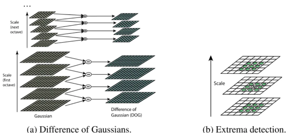
D(x,y,σ) =L(x,y,kσ)−L(x,y,σ) (3.2) The difference-of-Gaussian function is obtained by successively subtracting adjacent scale-space representations of the same image that differ by a constant factork>1 in scale as seen in (3.2). In this context, an octave is said to be completed every time the current scale is doubled with respect to the original scale. At the end of each octave the image is downsized and the process is carried on forming a pyramid representation as seen in Figure 3.1a extracted from [37]. Once the pyramid of DoG is available, the algorithm identifies the local maxima and minima in both scale and in space, performing a total of 26 comparison per point as seen in Figure 3.1b, obtained from the original article. In its original formulation, the number of scales used for searching these extrema was set to three, so that a total of five DoG representations were necessary for finding extrema over these central scales, which in turn requires six scale-space representation of images for each octave.

The precise locations of these extrema are further refined by fitting a 3D quadratic surface to the local points, which was shown to improve matching and keypoint stability [44]. Finally, unstable keypoints having low contrast or belonging to edges are eliminated.

It is worth mentioning that the difference-of-Gaussian gives an approximation to the scale-normalized Laplacian of Gaussianσ2∇2Gfunction whose minima and maxima have been verified experimentally to give more stable features with respect to other detectors such as Hessian and Harris [45].

3.1.2

SIFT Feature Extraction

SIFT descriptor achieves rotation invariance by assigning a dominant orientation for each keypoint. This is done by first extracting magnitude and angle of the gradients inL(x,y,σ)closest to the extremum found, as seen in (3.3) and (3.4) respectively. A 36-bin orientation histogram is then generated by quantizing the angles with steps of 10° and weighing each sample by the gradient’s magnitude and a gaussian-weighted mask centered around the extremum. The bin containing the maximum weighted

(30)

Scale (first octave) Scale (next octave) Gaussian Difference of Gaussian (DOG) . . .

Figure 1: For each octave of scale space, the initial image is repeatedly convolved with Gaussians to produce the set of scale space images shown on the left. Adjacent Gaussian images are subtracted to produce the difference-of-Gaussian images on the right. After each octave, the Gaussian image is down-sampled by a factor of 2, and the process repeated.

In addition, the difference-of-Gaussian function provides a close approximation to the scale-normalized Laplacian of Gaussian,σ2_∇2_{G, as studied by Lindeberg (1994). Lindeberg}

showed that the normalization of the Laplacian with the factorσ2_{is required for true scale}

invariance. In detailed experimental comparisons, Mikolajczyk (2002) found that the maxima and minima ofσ2_∇2_G_{produce the most stable image features compared to a range of other}

possible image functions, such as the gradient, Hessian, or Harris corner function. The relationship betweenDandσ2_∇2_G_{can be understood from the heat diffusion}

equa-tion (parameterized in terms ofσrather than the more usualt=σ2_):

∂G ∂σ=σ∇

2_G.

From this, we see that∇2_G_{can be computed from the fi nite difference approximation to}

∂G/∂σ, using the difference of nearby scales atkσandσ: σ∇2_G₌∂G ∂σ≈ G(x, y, kσ)−G(x, y, σ) kσ−σ and therefore, G(x, y, kσ)−G(x, y, σ)≈(k−1)σ2 ∇2_G.

This shows that when the difference-of-Gaussian function has scales differing by a con-stant factor it already incorporates theσ2_{scale normalization required for the scale-invariant}

6

(a) Difference of Gaussians.

Scale

Figure 2: Maxima and minima of the difference-of-Gaussian images are detected by comparing a pixel (marked with X) to its 26 neighbors in 3x3 regions at the current and adjacent scales (marked with circles).

Laplacian. The factor(k−1)in the equation is a constant over all scales and therefore does not influence extrema location. The approximation error will go to zero askgoes to 1, but in practice we have found that the approximation has almost no impact on the stability of extrema detection or localization for even signifi cant differences in scale, such ask=√2.

An effi cient approach to construction ofD(x, y, σ)is shown in Figure 1. The initial image is incrementally convolved with Gaussians to produce images separated by a constant factorkin scale space, shown stacked in the left column. We choose to divide each octave of scale space (i.e., doubling ofσ) into an integer number,s, of intervals, sok = 21/s_.

We must produces+ 3images in the stack of blurred images for each octave, so that fi nal extrema detection covers a complete octave. Adjacent image scales are subtracted to produce the difference-of-Gaussian images shown on the right. Once a complete octave has been processed, we resample the Gaussian image that has twice the initial value ofσ(it will be 2 images from the top of the stack) by taking every second pixel in each row and column. The accuracy of sampling relative toσis no different than for the start of the previous octave, while computation is greatly reduced.

3.1 Local extrema detection

In order to detect the local maxima and minima ofD(x, y, σ), each sample point is compared to its eight neighbors in the current image and nine neighbors in the scale above and below (see Figure 2). It is selected only if it is larger than all of these neighbors or smaller than all of them. The cost of this check is reasonably low due to the fact that most sample points will be eliminated following the fi rst few checks.

An important issue is to determine the frequency of sampling in the image and scale do-mains that is needed to reliably detect the extrema. Unfortunately, it turns out that there is no minimum spacing of samples that will detect all extrema, as the extrema can be arbitrar-ily close together. This can be seen by considering a white circle on a black background, which will have a single scale space maximum where the circular positive central region of the difference-of-Gaussian function matches the size and location of the circle. For a very elongated ellipse, there will be two maxima near each end of the ellipse. As the locations of maxima are a continuous function of the image, for some ellipse with intermediate elongation there will be a transition from a single maximum to two, with the maxima arbitrarily close to

7

(b) Extrema detection.

Fig. 3.1 SIFT detection: Keypoints are defined as extrema in the scale-space difference-of-Gaussian function both locally and in scale.

sum of magnitudes defines the keypoint’s orientation which, along with images coordinatesx,yand scaleσ, completely defines a keypoint. However, if the second highest weight sum of gradient magnitude is over 80% of the maximum value, a second keypoint is defined, so that a single extremum can generate more than one keypoint. m(x,y) = q (L(x+1,y)₋L(x₋1,y))2+ (L(x,y+1)₋L(x,y₋1))2 (3.3) θ(x,y) =arctanL(x,y+1)−L(x,y−1) L(x+1,y)−L(x₋1,y) (3.4)

For each one of these detected keypoints, the SIFT descriptor will then generate a 128-dimension vector to be used during matching. This is done by considering image’s gradients at a 16x16 pixel neighborhood centered around the keypoint’s location and scale and rotated relative to the keypoint’s orientation. Much like when defining the keypoint orientation, the gradient’s magnitudes are weighted using a circular gaussian-weighted mask centered at the keypoint value as depicted in Figure 3.2a. However, instead of defining a global histogram of orientations, the descriptor divides the 16x16 neighborhood into 4x4 subregions of 4x4 pixels. For each subregion an 8-bin orientation histogram is generated as seen in Figure 3.2b. These 16 histograms are then concatenated into a 128-dimension vector, and finally the descriptor vector is unit normalized after all dimensions have been clamped at

(31)

3.1 Scale Invariant Feature Transform (SIFT) 15

(a) Weighted Gradients (b) Histogram Gradients

Fig. 3.2 SIFT descriptor generation: A 16x16 pixel grid is center at the detected keypoint. For each 4x4 subregion the descriptor generates an 8-bin orientation histograms.

0.2. This is an upper bound empirically found to reduce the effects of non-linear illumination.

3.1.3

SIFT Feature Matching

In the context of object recognition, an object present in a query imageqis said to be found in a candidate imagedif a certain number of features inqcorrectly match those ind. Matching of SIFT features is done by evaluating the pairwiseℓ2distances

between all feature vectors in the query image and all feature vectors in the candidate image. Each keypoint inqis then initially associated to the closest keypoint ind.

The existence of similar feature vectors in either set of features may lead to erroneous feature association. In order reduce the number of incorrect matches generated from similar features vectors in d the distance to the second closest keypoint is also taken under consideration. If the ratio between the distance to the closest and the distance to the second closet keypoint indis larger than 0.8 these features are no longer considered a match.

As in the case of Visual Odometry, the number of incorrect matches can be further reduced by selecting subsets of matching features that agree on a particular hypothesis of the visual transformation. In its original formulation SIFT uses the generalized Hough Transform [46] to find cluster of matched features that agree on change in scale, pixel coordinates and feature orientation. Other common approaches to robust parameter estimation for object recognition include the already mentioned

(32)

Random Sample Consensus (RANSAC) [47] and the Least Median of Squares (LMedS)[48].

3.2

MPEG Compact Descriptor for Visual Search

The ubiquity of digital cameras in devices connected to the Internet such as cell-phones, laptops and tablets has made these accessories the ideal platforms for de-veloping augmented reality and visual search applications, such as Google Goggles, Bing Vision, and Amazon Flow.

The existence of such applications, however, imposes new challenges to Content-Based Image Retrieval (CBIR) system, which must search over large datasets and respond with correct results within just a few seconds in order not to compromise the so called user experience. Moreover, visual search applications must also be bandwidth efficient since typical use cases include a user sending a query image or visual descriptors over limited Internet connection. In this scenario, it has been shown that sending locally extracted visual features instead of sending the entire image can significantly reduce the amount of data exchanged with the remote server [49, 50].

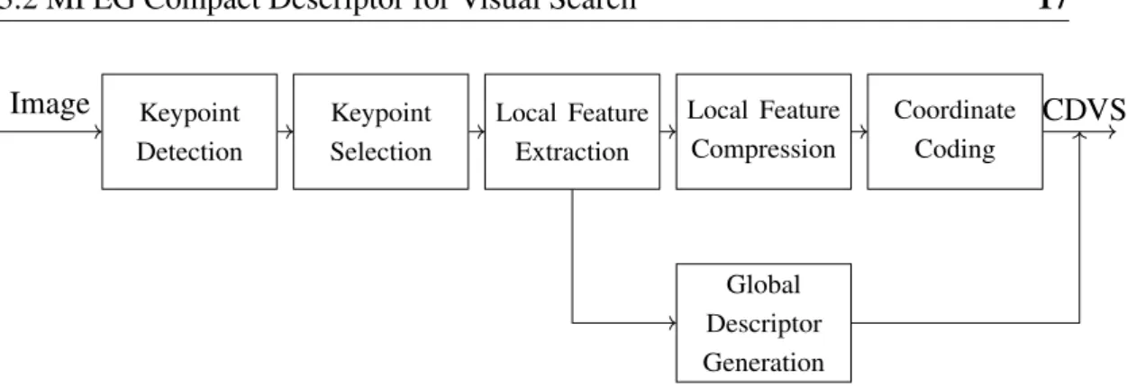
In response to these needs the Moving Picture Experts Group has recently com-pleted a new standard for image retrieval known as MPEG Compact Descriptor for Visual Search (CDVS) [1] designed specifically to allow for efficient and interop-erable visual search applications. An overview of the process by which features are detected, extracted and compressed according to the standard is represented in Figure 3.3. In this section we will briefly describe the key aspects of each block and highlight the optimization techniques developed for efficient image retrieval. A recent and complete overview of the standard and its history can be found in [51].

3.2.1

Image Preprocessing

In general, high resolution images are not required for correct object recognition and, most of the times, the use of large images just increases processing times. For these reasons, CDVS requires that input images have both horizontal and vertical dimension of at most 640 pixels. If one of the image’s dimensions is greater than

(33)

3.2 MPEG Compact Descriptor for Visual Search 17 Keypoint Detection Image _Keypoint Selection Local Feature Extraction Local Feature Compression Coordinate Coding CDVS Global Descriptor Generation

Fig. 3.3 MPEG Compact Descriptor for Visual Search pipeline.

this value, then the image must be resized, keeping the original aspect ratio, so that the largest of the two dimensions be equal to 640 pixels.

3.2.2

Keypoint Detection

Similarly to the SIFT detector, CDVS interest points are found using the scale-space representation of images. However, differently from SIFT, CDVS searches for points of maxima and minima using a Laplacian-of-Gaussian approach instead of difference-of-Gaussians. Moreover, CDVS approximates the Laplacian-of-Gaussian (LoG) function by using a low-degree polynomial known as ALP (A Low-degree Polynomial) as seen in (3.5) and (3.6)

ALP(x,y,σ) =σ3 3

∑

k=0 a_kF_k+σ2 3

∑

k=0 b_kF_k+σ 3

∑

k=0 c_kF_k+ 3

∑

k=0 d_kF_k (3.5) F_k=σ_k2L(x,y,σk)∗f (3.6)

where f is the discrete Laplacian operator matrix anda_k,b_k,c_kandd_kare coefficients defined by the standard. CDVS also defines procedures to refine the keypoint’s coordinate position to sub-pixel precision; to remove duplicated keypoints extracted at different octaves; and to assign an orientation to each keypoint.

When compared to SIFT feature detector, ALP detects extrema using a smaller number of pixel-neighborhood comparison. ALP first finds local extrema over the scale-space through the polynomial’s first derivative and then it compares each extremum with only 8 spatial neighbors. Also, as seen in (3.5), ALP requires only 4 image filtering operations per octave. Besides being a faster approximation of a

(34)

Table 3.1 Maximum descriptor length in bytes for each mode of compression. Compression mode 1 mode 2 mode 3 mode 4 mode 5 mode 6 Descriptor Length 512 B 1024 B 2048 B 4096 B 8192 B 16 386 B

LoG, the ALP detector has also been shown to retrieve more repeatable key points than the SIFT keypoint detector [52].

3.2.3

Keypoint Selection

Differently from the SIFT descriptor, CDVS does not generate an unbounded set of feature vectors for each detected keypoint. Instead, the CDVS feature extraction generates a bitstream that includes a subset of local features whose total length in bytes is upper-bounded according to one of the modes of compression listed in Table 3.1.

This upperbound implicitly limits the number of descriptors generated by an image and thus poses the question of which subset of keypoints should be used for extracting feature descriptors. Statistical studies on the probability of correctly matching pairs of local features [53] have helped answer this question by defining a measure of relevance for each keypoint. This measure is a function of the following keypoint characteristics:

• Scale where the keypoint was found.

• Keypoint response to the ALP feature detector. • Keypoint spatial distance to the center of the image.

• Ratio of the squared trace of the Hessian to the determinant of the Hessian, obtained during subpixel refinement.

• Second derivative of the scale-space function with respect toσ.

An indirect benefit of feature selection is that, by limiting the number of local fea-tures available in a CDVS bitstream, it reduces the time required for both extraction and matching of visual descriptors.

(35)

3.2 MPEG Compact Descriptor for Visual Search 19

Table 3.2 Number of selected transformed dimensions used by each mode of compression. Compression mode 1 mode 2 mode 3 mode 4 mode 5 mode 6

Number of dimensions 20 20 40 64 80 128

3.2.4

Local Feature Extraction

CDVS uses the SIFT descriptor as a starting point for its local descriptors. For each selected keypoint on the previous step, a 128 dimension vector is generated by computing the histograms of gradients relative to the keypoint’s orientation. The standard follows typical SIFT implementations [54] where each component of this vector is quantized to integer values between 0 and 255.

3.2.5

Local Feature Compression

Not all of SIFT dimensions will contribute to the final CDVS local feature. The standard first alternately applies two sets of linear transformations to each histograms of SIFT subregions (Figure 3.2b). According to the compression mode being used, the compression algorithm selects a specific subset of the transformed components to compose the local feature. The number of selected transformed components is reported in Table 3.2.

In order to allow for interoperability between modes, the order with which these components are selected was chosen so that the set of components of a more compressed mode is always a subset of the set of components of a less compressed mode.

Once the transformed components have been selected, each component is quan-tized to three values namely₋1, 0, and 1 and finally encoded into 10,0, and 11. The quantization levels for each component are defined in the standard’s normative lookup tables.

Coordinate Coding

The next step in the feature compression pipeline is to efficiently encode the coor-dinates of each keypoint. Coorcoor-dinates are usually represented using floating-point

(36)

precision, which becomes the bottleneck once the feature vectors have been quan-tized. CDVS uses a location histogram coding scheme [55] to identify clusters of features and efficiently make use of arithmetic coding.

3.2.6

Global Descriptor Generation

CDVS also defines a global descriptors which gives a general representation of the entire image based on the statistics of local features. This is obtained by first selecting up to 250 local features to whom reduce dimensionality using Principal Component Analysis (PCA). It then generates a Fisher Vector [56] representation using a 512 component Gaussian Mixture Model. CDVS further quantizes the global descriptor as to allow for fast Hamming-distance comparison [57].

3.2.7

CDVS Feature Matching

Local Features

Comparison between local features is performed with ℓ1-norm using XOR and

lookup tables, which is much faster thanℓ2-norm used by SIFT.

CDVS also considers the distance ratio r between the closest match and the second closest one, and defines a matchingscorefor each matching pair based on this distance ratio as seen in (3.7).

β =cosπr

2 (3.7)

Should more than one point from one image be associated to the same point in the other image, then whichever match scored lowest according to (3.8) is removed from the set of matching pairs. Based on this definition, the standard also suggests a metric of image similarity known aslocal scoredefined as the sum of the scores of all matching pairs.

local score=

N

∑

i=1

(37)

3.3 Other Visual Features 21

Geometric Consistency Check

The standard also describes a non-normative geometric consistency check algorithm called DISTRAT. The algorithm defines a goodness-of-fit test whose null hypothesis is based on the spatial distribution of incorrectly matched features. The algorithm has been shown to be many time faster than other robust parameter estimators such as RANSAC [58].

Global Descriptor

The similarity score between two global descriptors is referred to asglobal score

and it is a weighted correlation between the these descriptors. Theglobal scorecan be calculated efficiently using XOR and lookup tables. Since the global descriptor ignores the spatial positions of features in an image, its value for metric robotic navigation is very limited, hence it was not used in this work.

3.3

Other Visual Features

A plethora of visual detectors and descriptors has been suggested in the literature in the past 20 years. Here we give a brief overview of the most relevant ones to the field of robotic navigation. For a more complete survey of the subject we refer the reader to the works in [59, 15, 60].

• Harris: A popular corner detector that locally analyses the autocorrelation function of the image[61]. It defines the structure tensor in (3.9) wherew(u,v)

is a circular gaussian window.

A=

∑

u

∑

v w(u,v) " I_x2 I_xI_y I_xI_y I_y2 # (3.9)

A point in the image is defined to be a corner if the two eigenvalues ofAare large. In order to avoid having to calculate these values, Harris suggests using (3.10) with the tunable factork.

(38)

• Shi-Tomasi:A corner detector similar to Harris, but whose metric for detec-tion is the lowest among the eigenvalues ofA[62]. When compared to Harris, this metric is found to be more robust to affine transformation.

• FAST:The Features from Accelerated Segment Test [63] relies finds corners by searching for arcs around a pixel. This test allows for and average of just 3.8 pixel comparisons for each candidate.

• GLOH:The Gradient Location and Orientation Histogram [60] is an extension to SIFT, which uses a log-polar grind and PCA to reduce the dimensionality of the final descriptor.

• SURF:The Speeded Up Robust Features [64] is both a feature detector and descriptor developed to be a faster alternative to SIFT. It approximates the determinant of Hessian blob detector using Haar wavelet which can be ef-ficiently implemented using the integral image technique described in [65]. The feature descriptor is generated using Haar wavelet responses around the detected points, which can also be computed with integral images.

• CenSurE:The Center Surround Extremas [66] is a fast blob detector that computes the extrema of center-surround filters over multiple scales using the image’s original resolution for each scale. Center-surround filters are very coarse approximations of the Laplacian of Gaussian operator. The name derives from the high contrast between central and peripheral regions of the filter.

• BRIEF:The Binary Robust Independent Elementary Features [67] is a binary string feature descriptor whose individual bits are obtained by comparing the brightness of pairs of points around the keypoint position. Feature matching is fast as it is performed using Hamming distance.

• BRISK:The Binary Robust Invariant Scalable Keypoints[68] defines scale-space FAST-based detector which allows for rotation invariance in combination with a binary descriptor.

(39)

Chapter 4

Deep Learning for Object

Classification

In previous chapters we have described how visual features originally developed for object recognition and later optimized for large scale image retrieval can be used in the context of metric SLAM. This interoperability was possible mainly because these two tasks shared the same underlying assumption where places and objects are unique, rigid entities.

Unfortunately, this same assumption does not hold for the more general task of image classification where an image must be labeled according to a finite set of classes such asdog,human,airplane, etc. The difficulty in solving this task lies in the fact that labels encode semantics not immediately related to isolated image patches. In fact, classification can be interpreted as a complex function which must analyze the image as a whole and discard irrelevant information. For example, an image of a dog should be classified as a dog regardless of the dog’s race, pose or color; and a chair should be correctly classified regardless of its precise shape, and material. Early attempts to solve the problems of non-rigid deformations and intra-class variability include the use feature aggregation methods such as bag-of-visual-words [69, 70], and Fisher Vector [71, 72].

The bag-of-visual-words represents each image as a histogram of its quantized visual features. Usually Principal Component Analysis (PCA) is applied on a large amount of feature vectors obtained from a large dataset of images. K-means is then used over the dimensionality reduced features in order to generated a fixed dictionary.

(40)

Finally each feature in an image is represented using this dictionary and the entire image is represented as a histogram of occurrences. The Fisher Vector approach, on the other hand, first obtains a Gaussian Mixture Model (GMM) from a large number of feature vectors that will represent a global generative model of the features. Each image is then represented by the gradient of the log-likelihood of its set of features on the GMM, which in turn measure how individual parameters of the GMM should change to better accommodate the image’s feature distribution.

At this point we notice that both strategies rely on the extraction of visual features that were developed separately from the aggregation mechanism. In fact, the strategy of building intermediate representations on top of predefined features was so commonly used that famous object classification challenges like the ImageNet Large Scale Visual Recognition Challenge (ILSVRC) 2010 would provide“vector quantized SIFT features suitable for a bag of words" in order to “facilitate easy participation"1.

In this chapter we describe a family of Artificial Neural Networks, known as Convolutional Neural Networks (CNN), which have become the standard approach in object classification in past few years due to their great performance in solving such task. These networks reflect a new paradigm to machine learning known as Deep Learning, whose objective is tolearnhierarchical set of features directly from data and it is inspired by the early discoveries about the visual cortex [73]. We invite the interested reader to refer to the first chapters of [74] for a more thorough introduction to the Deep Learning, while a collection of important historical events in Deep Learning is reported in [75].

4.1

Artificial Neural Networks

An Artificial Neural Network (ANN) is a computational structure composed of interconnected elementary units called Artificial Neurons originally introduced by McCulloch and Pitts [76]. Their model of a neuron consisted of a set of identical weights, a fixed threshold, binary inputs and output, and an inhibitory signal. Under this model, a neuron would output 1 only if the inhibitor signal were inactive and the

1_{“Features."}_{Large Scale Visual Recognition Challenge 2010 (ILSVRC2010).}_{Stanford Vision} Lab. Web. 14 Jan. 2017

(41)

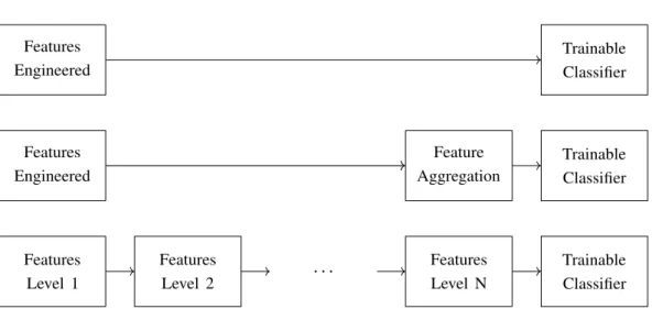
4.1 Artificial Neural Networks 25 Features Level 1 Features Level 2 . . . Features Level N Trainable Classifier Features Engineered Feature Aggregation Trainable Classifier Features Engineered Trainable Classifier

Fig. 4.1 The first row corresponds to original classic approach to object detection. The second row represents classic approach to object classification. Bottom row represent the Deep Learning approach where each feature level is learned.

weighted sum of inputs were greater than the fixed threshold. If either one of these conditions were not met, the neuron would output zero.

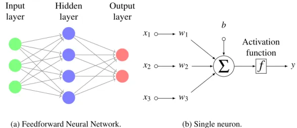
Rosenblatt’s perceptron [77] later improved this model by removing the inhibitor signal; allowing weights and bias to have different real values for each input; and finally, by providing an algorithm for learning those parameters. Today’s model of artificial neuron carries most of the perceptron’s characteristics except for its activation function, which no longer needs to be a binary threshold. A modern artificial neuron is depicted in Figure 4.2b, while examples of commonly used activation functions nowadays are seen in Figure 4.5.

The directed graph formed by the connections of neurons defines the network’s architecture. According to the presence or absence of cycles in such graph, an ANN architecture can be classified as either recurrent or feedforward neural network. Cycles in a network create a dependency of the current output on the values of previous inputs, which makes recurrent neural networks most useful when applied to long sequences that have some degree of temporal correlation, such as audio and text. Feedforward neural networks, on the other hand, are more suited for applications where sequences of inputs can be considered to be independent.

As we shall see, Convolutional Neural Networks for object classification are essentially feedforward ANNs, as seen in Figure 4.2a, but whose connections have been constrained to mimic the ones from the optic nerves to the visual cortex.

(42)

Hidden layer Input layer Output layer

(a) Feedforward Neural Network.

x₂ w₂

Σ

f

Activation function y x₁ w₁ x3 w3 b (b) Single neuron.

Fig. 4.2 Usual representation of a feedforward neural network and its associated artificial neuron model.

4.2

Convolutional Neural Networks

Convolution Neural Networks as known today has its roots in the handwritten character recognition system developed by Fukushima [78] known as neocognitron. Inspired by the structure of the mammalian visual cortex [73], the neocognitron was a hierarchical, multi-layered artificial neural network composed of alternating layers of simple cells (S-cells) and complex cells (C-cells). Each neuron in an S-cell layer is responsible for detecting a particular pattern in the previous layer and produce a “cell-plane" map containing the 2D position where the pattern was found. Layers containing C-cells were designed to provide a certain degree of shift invariance and activated if features in its vicinity were active.

Based on these ideas, Yann Lecun developed the LeNet-5 network for handwrit-ten digits classification [79] consisting of two alternating sequences of convolutional layers and pooling layers, followed by three fully-connected layers. The significance of LeNet-5 for the development of CNNs is twofold: First, it serves as the basic structure for most CNNs architectures, i.e. sequences of alternating layers of convo-lution and pooling followed by a few fully-connected layers, as seen in Figure 4.3, where the depth of a network is defined as the number of these non-linear layers; and second, it showed that CNNs could be trained using the efficient gradient-based learning method known as the backpropagation algorithm. In this section we will fo-cus on describing in depth each of the layers mentioned above, while the description of the backpropagation algorithm is postponed until the next chapter.

(43)

4.2 Convolutional Neural Networks 27

Conv. Pool Conv. Pool . . . FC FC

Fig. 4.3 Basic structure of a Convolutional Neural Network. A number of aternating convolu-tional and pooling layers is applied to the input for feature extraction followed by a sequence of one or more fully-connected layers.

4.2.1

Convolutional layers

Convolutional layers are the essential building-blocks in a CNN that are responsible for extracting features based on the principles ofshared weightsandlocality.

In a convolutional layer, inputs and outputs are arranged as sequences of 2D maps. Each neuron associated to an output is connected only to a small spatial neighborhood of all input maps. These local connections account forlocality in CNNs and forces features to represent spatial information.

Oftentimes features that meaningful in one region of the image are also mean-ingful over all parts of the image. This leads to the idea of shared weight, where neurons associated to the same output 2D map share the same set of weights. In this way, each output map is associated to a feature (set of weights) maps the spatial position where the feature was found, leading to the termfeature-map.

The number of maps in each sequence is referred to aschannels, much like the channels in color image. In fact, if the convolutional layer in question is the one immediately connected to input images, the number of input channels of the layer will be three for RGB images and one for gray scale images.

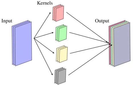
A closer look at the implementation of shared-weights and locality reveals that the output of a convolutional layer can be obtained by convolving the input with the set of shared weights, hence the name convolutional layer. Under this interpretation, each set of local weights is referred to as akerneland each kernel must have the same number of channels as the input signal. Finally we observe that, convolutions are performed only on thevalidspatial region of input maps, and that they may use strides different from one for computational purposes at the cost of loosing spatial resolution. This means that, considering square input maps of side

I, a kernel with spatial resolutionK, and a stride ofS, the final side of the output mapsO= (I₋K)/S+1 . In order to avoid continuous loss of spatial resolution

(44)

it is common practice to spatially pad the boarders of input maps. A common representation of Convolutional layers is seen in Figure 4.4.

Input

Kernels

Output

Fig. 4.4 Convolutional Layer: Each kernel performs channel-wise 2D convolutions to produce a single channel in the output set of feature-map.

4.2.2

Activation Functions

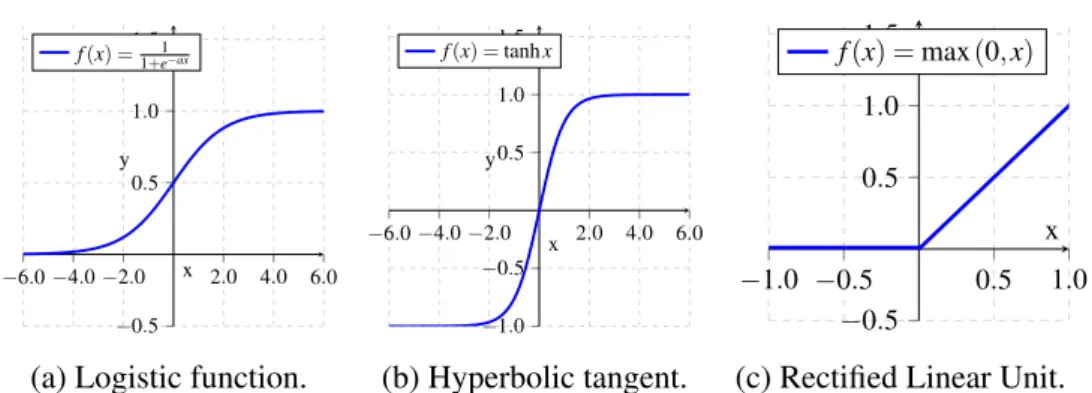
Although the modern definition of Artificial Neuron encompasses the use of activa-tion funcactiva-tions, common implementaactiva-tions of CNNs usually define them as separate layers. In Deep Learning, the activation function applied to the pre-activation stage of each neuron (weighted sum of inputs) need be non-linear. This allows for the network to represent complex function such as the “XOR" problem. The choice of non-linear activation function influences the network’s performance and are still subject of research today [80]. Following are the most commonly used activations in literature:

• Logistic function: The logistic function belongs to a family of “S" shaped functions known as sigmoid functions and it was the most commonly used activation function until recent years. It outputs values from 0 to 1 and it is a strictly increasing, differentiable function which shows near-linear behavior around zero and saturation over the extremes. As we shall see in the next chapter, linearity is important during training.

(45)

4.2 Convolutional Neural Networks 29 −6.0−4.0−2.0 2.0 4.0 6.0 −0.5 0.5 1.0 1.5 x y f(x) = 1 1+e−ax

(a) Logistic function.

−6.0−4.0−2.0 2.0 4.0 6.0 −1.0 −0.5 0.5 1.0 1.5 x y f(x) =tanhx (b) Hyperbolic tangent. −1.0 ₋0.5 0.5 1.0 −0.5 0.5 1.0 1.5 x y f(x) =max(0,x)

(c) Rectified Linear Unit. Fig. 4.5 Commonly used activation functions.

• Hyperbolic Tangent:For CNNs having many layers, the fact that the logistic function is not a zero-mean function will eventually cause later layers to work on the saturation region of the function [81]. This can be avoided by using the hyperbolic tangent which has zero mean and also belongs to the sigmoid function family and thus has the same desirable features.

• Rectified Linear Unit (ReLU):This is today’s most used and recommended activation function. It is a piecewise linear function that outputs 0 for negative values of pre-activation and the pre-activation value itself otherwise [82],[83, 84]. The rectified linear unit is not differentiable at the origin, but in practice this is not a problem.

4.2.3

Pooling Layer

Hubel and Wiesel’s notion of “complex cells" where the outputs of spatially close features are combined in order to achieve shift invariance and robustness to noisy input has been incorporated in what today is known as pooling layers. Common pooling layers usually act only on the spatial dimensions of feature maps so that the number of input and output channels in a pooling layer is the same. The importance of pooling operation in computer vision has been thoroughly investigated [85] and current state of the art networks use implement one of the following pooling schemes:

• Average pooling:Outputs the average over a small kernel window throughout the entire image. It was very common in the past for its simplicity.

(46)

• Max-pooling:Outputs the maximum value of a small kernel window through-out the entire image. It is by far today’s most used pooling layer.

• Fractional Max-Pooling:Much like convolutional layers, pooling-layers can be used with integer strides to produce subsampled feature maps. In order to reduce the loss in resolution cased by integer strides, the work in [86] proposes