Thank 7KH50 RXWSXWV 50,75 Citatio See th Version Copyri Link to you for do 0,75HVHDUF VRI50,78 5HVHDUFK5H on: is record i n: ght Statem o Published wnloading FK5HSRVLWR QLYHUVLW\UHV HSRVLWRU\KWWSUHVHDUFKEDQNUPLWHGXDX in the RMI ment: © d Version: this docum RU\LVDQRSH VHDUFKHUV IT Researc ment from HQDFFHVVG ch Reposit the RMIT R GDWDEDVHVK ory at: Research R KRZFDVLQJW Repository WKHUHVHDUF FK
PLEASE DO NOT REMOVE THIS PAGE
Lee, E, Fung, I, Tam, V and Arashpour, M 2014, 'A fully autonomous kernel-based online learning neural network model and its application to building cooling load prediction', Soft Computing, vol. 18, no. 10, pp. 1999-2014.
https://researchbank.rmit.edu.au/view/rmit:27367
Accepted Manuscript
Springer-Verlag Berlin Heidelberg 2013
A fully autonomous kernel-based online learning neural
network model and its application to building cooling load
prediction
E.W.M. Lee∙I.W.H. Fung∙V.W.Y. Tam∙M. Arashpour
Abstract
Building cooling load prediction is critical to the success of energy-saving measures. While many of the computational models currently available in the industry have been developed for this purpose, most require extensive computer resources and involve lengthy computational processes. Artificial neural networks (ANNs) have recently been adopted for prediction, and pioneering works have confirmed the feasibility of this approach. However, users are required to predetermine an ANN model’s parameters. This hinders the applicability of the ANN approach in actual engineering problems, as most engineers may be unfamiliar with soft computing. This paper proposes a fully autonomous kernel-based neural network (AKNN) model for noisy data regression prediction. No part of the model’s mechanism requires human intervention; rather, it self-organises its structure according to the training samples presented. Unlike the other existing autonomous models, the AKNN model is an online learning model. It is particularly suitable for online steps-ahead prediction. In this paper, we benchmark the AKNN model’s performance according to other ANN models. It is also successfully
E.W.M. Lee ()∙I.W.H. Fung
Department of Civil and Architectural Engineering, City University of Hong Kong, Kowloon Tong, Hong Kong
E-mail: [email protected] V.W.Y. Tam
School of Computing, Engineering and Mathematics, University of West Sydney, Locked Bag 1797, Perth, NSW 2751, Australia
M. Arashpour
applied to predicting the cooling load of a commercial building in Hong Kong. The occupancy areas and concentration of carbon dioxide inside the building are successfully adopted to mimic the building’s internal cooling load. Training data was adopted from actual measurements taken inside the building. Its results show reasonable agreement with actual cooling loads.
Keywords: Artificial neural network, building cooling load, kernel regression.
1 INTRODUCTION
Data regression is a major task of artificial neural network (ANN) models. Traditional ANN models (e.g., multilayer perceptron (MLP) (Rosenblatt, 1962), radial basis function (Broomhead & Lowe, 1988), general regression neural network (Specht, 1991), etc.) are widely adopted in different industrial applications. However, one major shortcoming of these models is that the user is required to determine the network structure and/or parameters via trials. In addition, the models can only be used as offline training models. In other words, a model’s structure cannot be updated by a single new training sample alone. Rather, it must be updated by a new training sample together with all of the training samples used previously, which greatly decreases the model’s applicability. Realising this limitation, Saad and Solla (1995) developed the online learning version of the MLP model by adopting the error function as an activation function of the neuron. Further, Freeman and Saad (1997) proposed an online RBF model. While these traditional ANN models were upgraded to online learning (Saad, 1998), they were not developed to operate in a noisy environment. The Nadaraya-Watson estimator (Nadaraya, 1964; Nadaraya-Watson, 1964) shown in Equation (1) is one of the most widely adopted templates for kernel-based regression model development, where
( ) = ( /ℎ) is the kernel function with a smoothing parameter ℎ, and and are the centre and label of the kernel, respectively.
( ) =∑∑ ( − )
( − ) (1)
Until now, many kernel-based regression models (Cai, 2001; Lee et al., 2004; Meinicke et al., 2005; An et al., 2011; Kramer & Gieseke, 2012) have been developed based on the Nadaraya-Watson estimator. Such kernel-based regression and classification models have also been widely adopted in building engineering (Chen et al., 2012; Yuen et al., 2006). The powerful general regression neural network (GRNN) model (Specht, 1991) also adopts the Nadaraya-Watson estimator. As it treats each training sample as a kernel, its major shortcoming is the huge model structure required in the case of a large-sized training batch. However, this limitation can be overcome by the introduction of a clustering pre-processor. Various clustering processors (Bezdek, 1980; Kohonen, 1990; Carpenter et al., 1991) have been proposed to cluster training samples into a smaller number of kernels. In our previous work (Lee et al., 2004), the GRNN model was also modified, and an online learning version known as the GRNNFA model was developed by implementing Fuzzy ART (Carpenter et al., 1991) as the pre-processor for the online clustering of the samples into a smaller number of kernels. The clustering is only carried out in the input domain of the samples. This leads to the GRNNFA’s major deficiency, i.e., it ignores the correlation between the input and output domains in the clustering process. Further, similar to other online learning models, the GRNNFA model’s performance is subject to the choice of parameters in the Fuzzy ART model and the initial width of a newly created kernel.
Kernel width estimation is crucial to the performance of kernel machines. Researchers have developed different heuristics to determine kernel widths. Based on work by Nakayama et al. (2002), Kitayama et al. (2012) developed a simple radial basis function (RBF) expression to determine the width of each kernel: = , ( ) ⁄ ( − 1) / , where is the width of kernel , , is the maximum distance from the centre of kernel to the most remote sample in the training dataset and and are the total number of kernels and the dimension of the space, respectively. While this expression greatly simplifies kernel estimation, kernels are assumed to be spherical in shape, and the estimation does not take into account the information of other kernels. Hence, it is not an optimised approach. Further, the user predefines the number of kernels, restricting the model to operating in offline mode only. Zhou et al. (2011) recently applied Bayesian information criteria together with differential evolution to detect the optimum number of kernels of an RBF and its global kernel width. While the result was encouraging, the model is restricted to offline learning. Singh and Príncipe (2012) developed an online kernel-width tuning approach that adaptively adjusts kernel widths to minimise the difference between the probability density distribution estimated by Parzen kernels and the actual distribution. Kullback-Leibler divergence is adopted to measure the difference in the distributions. Although this is an online training model, it is not an incremental growth model, and the user is required to predefine the number of kernels. Cervellera et al. (2012) recently improved the efficiency of kernel models by introducing the N-local neighbouring approach to tuning kernel width according to the neighbouring samples. This significantly decreases the time required to optimise the kernel width, and prediction accuracy is retained.
None of these recently developed kernel models are fully autonomous. Each has its own model parameters that require user tuning. This creates a hurdle for users who are unfamiliar with soft computing in using ANN models. Recently, Ferreira and Alves da Silva (2011) proposed an autonomous neural network model combining the automatic input selection developed from chaos theory and the training of MLP and relevance vector machine (RVM) models by Bayesian inference. The priori probabilities of the hyper-parameters of the model are described by non-informative gamma distributions and iteratively estimated by the principle of evidence maximization. Ferreira and Alves da Silva (2012) also applied the RVM model for short-term electrical loading forecasting. Their approach does not require human intervention in model training. However, it is an offline learning model. That is, when a new sample is available, the model should be trained again not only by this new sample but together with all of the previous collected samples. It restricts the model to be applied in online forecasting.
We propose a kernel-based incremental growth neural network model to overcome this hurdle. It is a fully autonomous ANN online learning model that does not require users to predefine any model structure or parameter.
The structure of this paper is as follows. Section 2 details the mechanism of the proposed autonomous kernel-based neural network (AKNN) model. The performance of the AKNN model is benchmarked in Section 3. Section 4 applies the AKNN model to predicting the cooling load of a commercial building in Hong Kong. Section 5 concludes the paper.
2 DEVELOPMENTOFTHEAKNNMODEL
The AKNN model is designed to be an online learning model. It is also an incremental growth model with a structure that grows autonomously according to training sample information. When a sample = , (where ∈ ℝ and ∈ ℝ are the respective input vector and scalar output of the sample ) is presented to the model, it is clustered according to the criteria of our proposed two-tier clustering approach to one of the model’s numbers of kernels (i.e., ). The kernels are designed to be correlated hyper-ellipsoidal Gaussian in shape (i.e., no restriction is imposed on the covariance terms) as follows, where and are the position vector and covariance matrix of the kernel , respectively.
( ) = 1
(2 )( )/ / −
1
2 − ( − )⊺ (2)
If none of the kernels satisfies the clustering criteria, a new kernel is created to code the new sample by our proposed nearest-neighbour approach. A probability density function in the joint input and output space is established by applying the Parzen density estimator (Parzen, 1962) to the kernels. In the course of model training, the probabilistic density function changes dynamically in response to the training sample presentation. For model prediction, the model’s output is determined by evaluating the expected conditional mean of the probability density function in terms of the input vector. The AKNN model’s mechanism is described as follows.
2.1 Model initialisation
The AKNN model is initialised to create kernels for the clustering process. It requires two training samples (e.g., and ), which are the centres of two initial kernels:
and . The widths of the two kernels are identical and taken to be half of the Euclidean distance between the centres of two kernels that are initially hyper-spherical in shape, as shown in Equation (3).
= =| − |
2 ∙ (3)
When a new sample is presented to this initialised model, the model tries to cluster it into either of the existing kernels according to our developed two-tier approach as follows.
2.2 The two-tier clustering approach
This clustering approach consists of two tiers. Any sample to be clustered into either of the model’s existing kernels must pass through this two-tier test.
2.2.1 Nomination
The first tier is called nomination. When a new sample = , is presented to the AKNN model, it nominates one of the total numbers of the existing kernels (i.e., ) to which the new sample is to be clustered using the Bayesian approach. When the sample is presented to the AKNN model, kernel (i.e. , 1 ≤ ≤ ) is nominated by Equation (4), in which the value of ( ) is practically neglected because it is a constant. The value of is approximated by = ∑ , where is the number of training samples clustered into kernel .
= ,where = | ( ) (4)
The second tier is called confirmation. The nominated kernel is further examined by the second tier of clustering before confirmation. It is believed that when a sample is clustered into a kernel, the kernel’s information after including the sample should be clear and any uncertainty should be reduced. The uncertainty of kernel is represented by the differential entropy (Ahmed & Gokhale, 1989) of kernel , which can be determined by Equation (5).
= (2 ) . (5)
The nominated kernel is said to be confirmed if the condition in Equation (6) is satisfied. That is, the uncertainty of kernel is reduced after the inclusion of the new sample.
< (6)
If the clustering is confirmed, kernel is updated to include the new sample according to Equation (7), where , and are the number of samples, centre and covariance matrix of , respectively. The superscripts old and new represent the state of the variables before or after the inclusion of the new sample, respectively. This kernel update is a classical approach which retains the statistical integrity of kernels.
= + 1 = − 1 + = − 1 + − ⊺ − + − 1 − ⊺ − (7)
If the nominated kernel does not satisfy condition (6), kernel is reset; that is, the value of is set to zero and the next kernel is nominated again by Equation (4).
2.3 Kernel creation
During the AKNN model’s two-tier clustering process, if none of the existing kernels satisfies both conditions (5) and (6) in response to the presentation of a new training sample , the model creates a new kernel ( , , ) to code this new training sample. In some clustering approaches (Lim & Harrison, 1997; Lee et al., 2004; Singh & Markou, 2004), the new sample is taken as the kernel centre, , and an initial uniform width is manually assigned to the created kernel as described in Equation (8). However, this approach creates hurdles for the actual online operation of the model, as all of the training samples should be used in the trials to determine the appropriate kernel width.
= 1 =
= (8)
An approach that adopts the nearest neighbour concept is proposed to determine the kernel width autonomous of the nearest kernel’s information. Similar to other clustering approaches, the initial widths of new kernels are assumed to be uniform. The improved probabilistic neural network (PNN) developed by Cain (1990) also assumed that all kernels are hyper-spherical in shape but different in kernel widths. He proposed that the probability density estimate at a point should be significantly influenced by more than one sample but not by a large number of them. Therefore, the larger the number of samples and the denser these points, the smaller the kernel width must be for best performance. Therefore, the kernel width of a class is continuously updated and taken to be proportional to the average minimum distance between samples in the same class. By this approach, the width of each kernel no longer represents the variance of the samples of the same class. Applying this ‘adjusted’ kernel width to the PNN model
for Bayesian classification may defeat the integrity of the overall Bayesian approach. In our model, we propose to initialize the width of a new created kernel by Equation (9) that the initial kernel width is taken to be the shortest distances from the new sample s
to the widths of the nearest existing hyper-ellipsoidal Gaussian kernels. In the online learning process, the kernel width is updated by Equation (7). It is a classical approach which retaining the overall integrity of the Bayesian approach.
= min min − where − − ⊺ = 1 and = 1,2, ⋯ , (9)
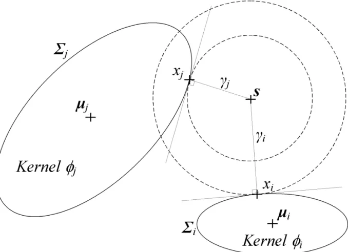
Fig. 1 provides an example. Assume that there are only two kernels in the domain. Points and are the tangent points of the new hyper-spherical kernel and the existing hyper-ellipsoidal kernels and , respectively. In this example, is the minimum shortest distance from the new kernel to the existing kernels. Therefore, the value of is taken to be the uniform width of the new kernel. The Lagrange multiplier is adopted to determine the width of new kernel . Assume that is the new sample and taken to be the centre of the new kernel, that and are the respective centre and width of existing kernel and that is the tangent point of the new kernel and existing kernel . The objective is to minimise the width of the new kernel tangential to the width of the existing kernel , as described in Equation (10).
Maximise − − − ⊺with constraint − − ⊺= 1 (10)
According to Equation (10), the Lagrange function Λ is set in Equation (11) according to the preceding criteria, where is the Lagrange multiplier.
The extremes of function Λ can be obtained by ∇Λ = 0 (i.e., ∇ Λ = 0 and ∇ Λ = 0). By evaluating ∇ Λ = 0, we arrive at Equation (12).
− = − − (12)
By evaluating ∇ Λ = 0, we arrive at Equation (13).
− − ⊺ = 1 (13)
Equation (14) is obtained by putting Equation (12) into Equation (13).
− − − − ⊺= 1 (14)
Equation (14) is simplified to Equation (15), from which the two possible values of can be obtained.
= ± − (15)
The two possible values of correspond to the shortest and longest distances from the new sample to the kernel . The two possible locations of can be obtained from Equation (12), and the shortest distance from the new sample to the kernel can also be obtained. A similar approach is applied to obtain the shortest distances
from the new sample to all of the existing kernels. The minimum shortest distance (i.e., min ) is taken as the initial uniform width of the new kernel.
2.4 Model prediction
In a regression task, the predicted result can be approximated by the expected conditional mean of a given input vector , which can be evaluated from the joint continuous probability density function ( , ) by Equation (16), where and are the input vector and scalar output of the underlying function , respectively.
( ) = ( , )
( , ) (16)
Parzen (1962) proposed a nonparametric estimation of probability density function ( , ) from the information of available samples using the kernel approach. The probability density function can be approximated by Equation (17), where the kernel, ( ), is defined in Equation (2).
( , ) = 1 ( , ) (17)
By applying Equation (17) to Equation (16), the expected conditional mean can be estimated by Equation (18).
( ) =∑ ( , )
∑ ( , ) (18)
The integral at the denominator of Equation (18) can be evaluated by Equation (19).
( , ) = ( ) (19)
The integral at the numerator of Equation (18) can be evaluated by the probabilistic approach as follows. Let ( ) = arg max ( , ) be the mean of the distribution ( , ) at location . The numerator of Equation (18) can then be evaluated as follows.
( , ) = − ( ) + ( ) ( , )
= − ( ) ( , ) + ( ) ( , )
= 0 + ( ) ( )
By putting Equations (19) and (20) back into Equation (18), the expected conditional mean can be evaluated by Equation (21).
( ) =∑ ( ) ( )
∑ ( ) (21)
The value of ( ) in Equation (21) can be obtained by putting the value of into kernel . The value of ( ) can be evaluated by setting the derivative of ( ) in Equation (21) in terms of zero. The result is shown in Equation (22).
( ) = , −
∑ − ,
,
(22)
where , are the elements in the last row of the inverse of covariance matrix as follows. = , , ⋯ , , , ⋯ , ⋮ ⋮ ⋱ ⋮ , , ⋯ , (23)
The expected conditional mean can then be evaluated by Equations (21) and (22).
3 EXPERIMENTALSTUDY
3.1 Noise-corrupted sine curve
We adopted the noise-corrupted sine curve benchmarking problem (Lee, 2011) to evaluate the AKNN model’s performance. A clean sine curve = ( ) was created within the domain [0,2 . One hundred samples were randomly extracted from the sine curve, with Gaussian noise (0,0.2) added into the sample output. These 100 noise-corrupted samples were used as the AKNN model’s training samples. The trained model was applied to reconstruct the sine curve. Test samples were extracted from the clean
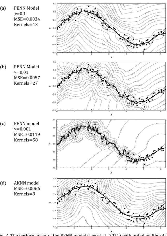
sine curve, with sample inputs taken from = 0 to 2 with step 0.01. The test samples numbered 629 in total. The trained model was applied to the 629 samples to obtain the 629 predicted outputs. The model’s performance was quantified using the mean squared error (MSE) of the 629 predicted values and sample outputs. Four tests were conducted. In the first three tests, the probabilistic-entropy-based neural network (PENN) model (Lee, 2011) was applied to reconstruct the sine curve according to the three different settings of the initial uniform kernel width (i.e., 0.1, 0.01 and 0.001). The AKNN model was adopted in the fourth test to reconstruct the sine curve. The results of the four tests were compared with the clean sine curve, and the MSEs were evaluated to compare the performances of the PENN and AKNN models as shown in Fig. 2. The PENN model’s performances with different initial kernel width settings (i.e., 0.1, 0.01 and 0.001) are depicted in Fig. 2(a)-(c). As the AKNN model does not require any model parameters, only one predicted result was produced, as shown in Fig. 2(d). The MSE of the AKNN model’s prediction is 0.0066, which is lower than that of the PENN model with an initial width of 0.001 (i.e., 0.0119), but higher than the original PENN model with initial widths of 0.1 and 0.01 (i.e., 0.0034 and 0.0057, respectively). For the PENN model, we can see that the trials must be carried out to achieve the optimum setting of the initial uniform kernel width. The AKNN model eliminates this deficiency, dynamically determining the kernel width according to the information of its neighbouring kernels. Fig. 2(d) demonstrates the ability of the AKNN model in the task of noisy data regression. Although the AKNN model is not the best model to use in this benchmarking problem, it can reasonably reconstruct the sine curve, is fully autonomous and requires no human intervention in the model training. The AKNN model also created a lower number of kernels compared with that of the PENN models with different initial kernel widths.
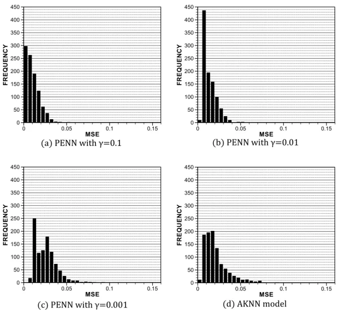
As both the PENN and AKNN models are online training models, their performances are sensitive to the order in which samples are presented in the model training. Therefore, we further investigated their performances using the statistical approach as follows. In each of the four tests, 1,000 trials were carried out using the same dataset; however, the model training samples were presented in a random order. After the trials, 1,000 MSEs were obtained from each test. Fig. 3 shows the distributions of the MSEs in the 1,000 trials in each test. Given that the 1,000 MSEs were bounded by a range [0, ∞), they were assumed to follow a log-normal distribution. To statistically evaluate the performances of the four tests, a left-tailed 95% confidence limit of the log-normal distribution of each test was evaluated. These are listed in Table 1, representing the models’ maximum MSEs with a 95% confidence level. It is shown that the AKNN model’s result (i.e., 0.0484) is higher than that of the PENN model with γ = 0.1 and 0.01 (i.e., 0.0275 and 0.0292, respectively) but lower than that of the PENN model with γ = 0.001 (i.e., 0.0484). In terms of this benchmarking problem, the AKNN model neither outperformed nor underperformed the PENN model. However, the AKNN model is fully autonomous; it does not require any trial to determine its parameter. Further, the AKNN model creates the minimum number of kernels.
3.2 Chaotic time series prediction
The chaotic time series used in this experimental study was created by the following Mackey-Glass differential delay equation (Mackey & Glass, 1977), of which (0) = 1.2 and = 17 for 0 ≤ ≤ 2000 and ( ) = 0 for < 0. The fourth-order Runge-Kutta method was used to obtain the system’s numerical solution.
( ) = 0.2 ( − )
1 + [ ( − ) − 0.1 ( ) (24)
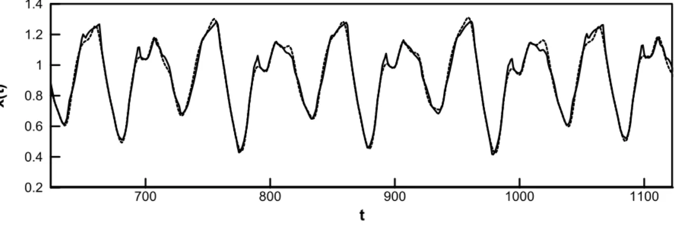
One thousand samples were extracted from = 124 to 1,123. The samples are plotted in Fig. 4 for illustration. The samples from = 124 to 623 (i.e., the first 500 samples) were used as training data, and the samples from = 624 to 1,123 (i.e., the remaining 500 samples) were used as testing samples. As this is a time series, the training samples were presented sequentially to the AKNN model.
The AKNN model created 14 kernels after the model training. The prediction on the testing samples is shown in Fig. 5. The predicted time series reasonably approximates the overall profiles of the original time series. However, minor deviations can be found at the peaks of the time series. The AKNN model’s performance is quantified by the root mean square error (RMSE) defined as follows, where and are the target and predicted values, respectively.
= ∑ ( − )
500 (25)
Table 2 compares the RMSE obtained by other models addressing the same benchmarking problem (Lee & Kim, 1994; Kim & Kim, 1997). The AKNN model’s RMSE is 0.026, which is higher than the genetic fuzzy predictor ensemble (Kim & Kim, 1997) but lower than the other models shown in Table 2. This indicates that while the AKNN model is not the best model, it performs reasonably well. However, it should be noted that among the models in Table 2, the AKNN model is the only one without parameters, and requires no human intervention in defining its structure and training.
4 APPLICATIONTOBUILDINGCOOLINGLOADPREDICTION
A cooling load is the quantity of heat energy that must be removed from a building to maintain the thermal comfort of the building’s occupants. It consists of two components: external and internal loads. The external load is the heat load resulting from meteorological factors (e.g., outdoor ambient temperature, humidity, sunshine, etc.), and the internal load is contributed by the building’s occupants and their ancillary activities (e.g., body temperature, lighting and operation of equipment, etc.). By predicting a building’s cooling load, a centralised air-conditioning system can optimise its operation (e.g., the operation sequencing of the chillers, intake of fresh air, etc.) to achieve the system’s optimum energy consumption.
In general, the main stream of energy analysis uses a forward approach in which energy predictions are based on a physical description of a building’s system, such as its geometry, the building’s construction details and the equipment and operation schedule of the heating, ventilation and air-conditioning (HVAC) systems. Most of the current energy analysis software such as BLAST (1992), DOE (2005), TRNSYS (2006) and ENERGYplus (2011) adopt this forward approach. However, establishing a simulation model is very time consuming and resource intensive, especially for complex mixed-purpose buildings with unregulated operating schedules. A number of pioneering researchers have alternatively used intelligent models for simulations and predictions in the field of building services engineering. Yuen et al. (2006) used the ANN approach to predict the temperature and velocity of hot gases passing through the doorway of a fire compartment. Soyguder and Alli (2009) applied a fuzzy inference system to predict the fan speeds and energy consumptions of HVAC systems. Kreider and Rabl (1994) used an MLP model to predict the pre-retrofit energy consumption of a building, which
they compared with the measured energy consumption of a retrofitted building. Yalcintas and Akkurt (2005) used a multilayered MLP to mimic the total chiller plant power of a 42-storey commercial building in downtown Honolulu, Hawaii. Yezioro et al. (2008) applied an MLP model with a Levenberg-Marquardt training algorithm to predict heating/cooling load consumption. Although these pioneering studies confirmed the feasibility of the ANN approach, all of the models require users to pre-define their structures and establish training parameters, which presents major hurdles.
4.1 Case study of a commercial building in Hong Kong
The building in the first case study is a prestigious high-rise commercial building located in the centre of Hong Kong. Its tenants include many multinational financial companies from around the world. The building has a floor area of more than 180,000 m2, and a curtain wall acts as its envelope. In this study, we applied the AKNN model to
predict the building’s cooling load. The model’s output was the cooling load, and its inputs were the external and internal load factors. We considered outdoor temperature, relative humidity, rainfall, wind speed, bright sunshine duration (i.e., the total time the sun’s intensity exceeded a predetermined threshold of brightness) and global solar radiation as the external load factors, and occupancy area and rate as the internal load factors. The occupancy area represented the total operating floor area of the building at any given hour according to the operating schedules submitted by the tenants. The occupancy rate reflected the number of occupants inside the building at any given hour. Because it is impractical to directly count the number of occupants inside a building, especially when dealing with some of the mega buildings in Hong Kong, we mimicked the occupancy rate pattern by estimating the concentration of carbon dioxide (CO2)
consumption of the primary air unit (PAU), which is a machine that drives fresh air into a building if the indoor CO2 concentration is high. The expected external and internal
loads that contributed to the building’s cooling load are summarised in Table 3.
Fig. 6 shows a typical profile of the commercial building’s cooling load in September and October 2008. From 4:00 on 6 September 2008 to 0:00 on 20 October 2008, a total of 1,053 samples were collected every hour. For the purposes of model training and evaluating the AKNN model’s performance, the first 80% of the samples (i.e., the 842 samples taken from 4:00 on 6 September 2008 to 5:00 on 11 October 2008) were used for network training, and the remaining 20% (i.e., the 211 samples taken from 6:00 on 11 October 2008 to 0:00 on 20 October 2008.) were hidden during the network training phase and kept in reserve as a testing set to evaluate the performance of the trained network. The result of the prediction is shown in Fig. 7. The AKNN model created only three kernels during the training phase. It was able to capture the general behaviour of the cooling load, showing it to be high during the day and low at night. Although prediction errors were still observed in the peaks and troughs of the profile, the irregularity of the building’s cooling load on 18 and 19 October 2008 was reasonably approximated by the AKNN model. The RMSE of the prediction is 856.14 kW. We further compare the performance of the AKNN model with the GRNN and Gaussian mixture (GM) models, as their structures are similar.
In the GRNN model, the samples were arranged as training, validation and test sets. The 211 testing samples (i.e., 20%) were the same as those used in the AKNN model prediction. The other 842 samples (i.e., 80%) used in the AKNN model’s training phase were randomly divided into training and validation sets at a 75% to 25% ratio, respectively. Therefore, the numbers of training and validation samples were 632 and
210, respectively. The GRNN model recruited each training sample as the centres of its kernels. Therefore, 632 kernels were created. All of the kernels were assumed to be identically spherical in shape. The global kernel width was determined by a genetic algorithm to achieve the best fit to the validation samples. The trained GRNN model was applied to the test samples. The prediction result is shown in Fig. 8, and the corresponding RMSE is 922.96 kW. Fig. 8 also shows the prediction result.
The AKNN model clustered the samples via its online training approach. To benchmark the AKNN model’s performance, the GM model was chosen for comparison. The GM model is an offline training model used for sample clustering. It clusters available samples into a predefined number of hyper-ellipsoidal Gaussian kernels using an expectation-maximisation (EM) algorithm. The same 211 samples used in the aforementioned tests were used as testing samples. The other 842 samples were clustered into the kernels of the GM model using an EM algorithm. For easy comparison, the number of kernels in the GM model was taken to be the same as that in the AKNN model (i.e., three kernels). Upon completion of the sample clustering, a prediction of the test samples was carried out by evaluating the expected conditional mean, as shown in Section 2.4. The prediction result is shown in Fig. 9, and the RMSE of the prediction is 429.53 kW. Fig. 9 also shows the result predicted by the GM model.
Due to the limited number of samples, cross validation approach is adopted to further evaluate the performances of the AKNN, GRNN and GM model. The procedures are detailed as follows. The total 1,053 samples used in the above evaluation are also used in this approach. In the first trial, we reserve 200 samples taken from the 1st sample to
the 200th sample as the testing samples. The other 853 samples are used to train the
200 testing samples to evaluate the first RMSE of the prediction. In the second trial, the next 200 samples taken from the 2nd sample to the 201st sample are reserved as the
testing samples and the other 853 samples are used for model training. The trained model is applied to the 200 samples to evaluate the second RMSE error. The process continues until the RMSE of the last 200 samples is obtained. Therefore, there are 854 RMSEs obtained upon the completion of this cross-validation approach. Fig. 10 shows the distribution of the RMSEs obtained from the AKNN, GM and GRNN models. They overlap with each other. It demonstrates their different performances in this case study. The maximum RMSE of the AKNN, GM and GRNN models are 1382kW, 786kW and 1093kW respectively. It shows that the performance of the GM is the best. Although the AKNN model shows higher prediction error than the GRNN model, the number of kernels created by the AKNN model (i.e., 3 kernels) was much less than that created by the GRNN model (i.e., 853 kernels). Although the GM model performs better than the other 2 models, the GM model adopts an offline learning approach (i.e., EM algorithm) which restricts its application for online forecasting. Also, the user must predetermine its number of kernels of the GM model.
4.2 Case study of a commercial building in Shanghai, China
This case study intends to determine the performance of the AKNN model in a different period. The data were collected from a prestigious super-high-rise commercial building in Shanghai, China with an aggregated floor area of 200,000 m2. The building’s envelope
comprises curtain walls. The AKNN model was adopted to predict the building’s cooling load based on meteorological factors including solar radiation, solar angles, outdoor dry bulb temperature and relative humidity. Data were collected every 15 minutes from 0:00 on 11 January 2013 to 10:15 am on 10 March 2013. Of the 5,610 samples collected,
the last 1,122 samples (i.e., 20% of the total) were reserved as test samples for evaluating the performance of the model trained by the 4,488 samples (i.e., 80% of the total). Similar to the previous case study, the AKNN, GRNN and GM models were adopted.
As the AKNN has no user-defined model parameters, the first 80% of the available samples were directly fed into the AKNN model without any model tuning. The AKNN model created 11 kernels. The trained AKNN model was applied to the remaining 20% of the available samples. The prediction result is shown in Fig. 11, and the corresponding RMSE is 129.8368 kW.
Similar to the previous case study, the first 80% of the available samples (i.e., the first 4,488 samples) were randomly divided into training and validation sets at a 75% to 25% ratio (i.e., 3,366 samples and 1,122 samples), respectively. The GRNN model recruited every sample of the training set as the kernel centres, thus creating 3,366 kernels. The GA tuned the global kernel width to achieve the minimum validation error. The trained GRNN model was applied to the remaining 20% of the available samples. The prediction result is shown in Fig. 12, and the corresponding RMSE is 178.16 kW. In the GM model training, the number of kernels was set at 11, the same as that created by the AKNN model. Similar to the GRNN model training, the 3,366 samples were used to form the 11 kernels using the EM algorithm. The GA then trained the kernel widths to achieve the minimum validation error. The trained GM model was applied to the remaining 20% of the available samples to evaluate its performance. The prediction result is shown in Fig. 13, and the corresponding RMSE is 128.15 kW.
In this case study, it is clear that the three models performed similarly to the way they performed in the previous case study. In terms of accuracy, the AKNN model performed better than the GRNN model but worse than the GM model. However, the AKNN model does not require any model parameter tuning. Further, the number of kernels it created was much less than that created by the GRNN model. In terms of applicability, the AKNN model is more user-friendly and able to produce a reasonable prediction result. Nonetheless, the AKNN model’s kernel width tuning is not an optimal approach. Rather, it involves a linear combination of Gaussian kernels, which may restrict the applicability of the model to linear problems.
Similar to the last case study, cross validation was also applied to further evaluate the performances of the AKNN, GRNN and GM models in this case study. The procedures are the same as the last case study. Total 5,610 samples are used and the number of test samples is taken to be 1,000 samples. At the end of the cross-validation, there are 4,611 RMSE obtained from each model. The results are plotted in Fig. 14. It is observed from this figure that the three distributions overlap with each other. The maximum RMSE of the AKNN, GM and GRNN models are respectively 135kW, 220kW and 185kW. It shows that the performance of the AKNN model, in this case study, is reasonably better than the other 2 models. However, it should be noted that the AKNN model does not require any pre-definition of model structure or parameter. In contrast, the GM model requires the user to pre-define the number of kernels of the model. Also, the number of kernels created by the AKNN model (i.e. 6 to 7 kernels) is much lower than that of the GRNN model (i.e. 4610 kernels) since it recruits every training sample as its kernel.
5 CONCLUSION
Cooling loads are important factors in a building’s energy management. Traditional approaches require extensive computer resources and lengthy computation time. Although pioneering works have demonstrated the feasibility of applying ANNs to predicting a building’s cooling load, users are required to determine the ANN model parameters on their own. This is the major hindrance to the ANN approach. This paper proposes a fully autonomous, kernel-based ANN model that does not require users to determine the initial uniform kernel width via trials. A kernel creation scheme adopts the nearest-neighbour approach to determine kernel widths. A Lagrange multiplier is applied to determine the shortest distance from the centre of a new kernel to the width of the nearest existing neighbouring kernel. We benchmarked the AKNN model’s performance with the PENN model via the noise-corrupted sine curve benchmarking problem. The results show that the AKNN model’s performance is comparable with that of the original PENN model. However, the AKNN model has the benefit of being fully autonomous and requiring no human intervention. A Mackey-Glass time series benchmarking problem was also applied to test the AKNN model’s performance. The results show that the AKNN outperforms most of the models discussed in studies by Lee and Kim (1994) and Kim and Kim (1997). In applying the AKNN model to building cooling load prediction, actual data were collected from an ultra-high-rise building in Hong Kong for training. The AKNN model was applied to predict the building’s cooling load, and it reasonably captured the cooling load’s profile, performing comparably with the GM and the GRNN modes. The AKNN also has its own limitations. The main deficiency of the present AKNN is the non-optimal selection of the kernel spread and the linear combination approach that it uses for modeling the underlying process. This confines its applicability to certain category of problems and limits its application to
problems that require non-linear modeling. However, the main advantage of the AKNN model is that it requires no user-set parameters; indeed, it is a fully autonomous model. No prior trial is required to determine the optimum setting of the initial kernel width before actual application. This is extremely useful for engineers who are unfamiliar with soft computing techniques. The online learning feature of the AKNN also facilitates the real-time or steps ahead time series predictions.
6 ACKNOWLEDGEMENT
This research was fully supported by a grant from the City University of Hong Kong (Project No. 7008028).
7 REFERENCES
Ahmed NA, Gokhale DV (1989) Entropy expression and their estimators for multi-variate distribution. IEEE Transactions on Information Theory 35(3):688-692. An SH, Heo G, Chang SH (2011) Detection of process anomalies using an improved
statistical learning framework. Expert Systems with Applications 38:1356-1363. Bezdek JB (1980) A convergence theorem for the fuzzy ISODATA clustering algorithms.
IEEE Transaction on Pattern Analysis and Machine Intelligence PAMI-2:1-8.
BLAST (1992) BLAST 3.0 User Manual. BLAST Support Office Department of Mechanical and Industrial Engineering, University of Illinois Urbana-Champaign, USA.
Broomhead DS, Lowe D (1988) Multi-variable functional interpolation and adaptive networks. Complex Systems 2:321-355.
Cai Z (2001) Weighted Nadaraya-Watson regression estimation. Statistics & Probability Letters 51:307-318.
Carpenter GA, Grossberg S, David BR (1991) Fuzzy ART: Fast stable learning and categorization of analog patterns by an adaptive resonance system. Neural Networks 4:759-771.
Cervellera C, Gaggero M, Macciò D (2012) Efficient kernel models for learning and approximate minimization problems. Neurocomputing 97:74-85.
Chen CS, Cheung MY, Wu YW (2012) Seismic assessment of school buildings in Taiwan using the evolutionary support vector machine inference system. Expert Systems with Applications 36(4):4102-4110.
DOE (2005) DOE release 2.2.2005. Hirsch, J. J. & Associate, Lawrence Berkeley National Laboratory Simulation Research Group, Berkeley, California, USA.
EnergyPlus (2011) EnergyPlus Manual Version 7.0. U.S. Department of Energy.
Ferreira VH, Alves da Silva AP (2011) Chaos theory applied to input space representation of autonomous neural network-based short-term load forecasting models, Sba Controle & Automação 22(6): 585-597.Ferreira VH, Alves da Silva AP (2012) Autonomous kernel based models for short-term load foresting. Journal of Energy and Power Engineering 6: 1984-1993.
Frederick MA (1996) Neuroshell 2 Manual, Ward Systems Group Inc., Maryland.
Freeman JA, Saad D (1997) Dynamics of on-line learning in radial basis function networks. Physical Review E 56(1):907-918.
Kim D, Kim C (1997) Forecasting time series with genetic fuzzy predictor ensemble. IEEE Transactions on Fuzzy Systems 5(4):523-535.
Kitayama S, Kita K, Yamazaki K (2012) Optimization of variable blank holder force trajectory by sequential approximate optimization with RBF network. The International Journal of Advanced Manufacturing Technology 61(9):1067-1083. Kohonen T (1990) The self-organizing map. Proceedings of the IEEE 78(9):1464-1480.
Kramer O, Gieseke F (2012) Evolutionary kernel density regression. Expert Systems with Applications 39:9246-9254.
Kreider JF, Rabl A (1994) Heating and Cooling of Buildings Chapter 8, McGraw–Hill, New York.
Lee EWM, Lim CP, Yuen RKK, Lo SM (2004) A hybrid neural network model for noisy data regression. IEEE Transactions on Systems, Man and Cybernetics – Part B 34(2):951-960.
Lee EWM (2011) An incremental adaptive neural network model for online noisy data regression and its application to compartment fire studies. Applied Soft Computing 11:827-836.
Lee SH, Kim I (1994) Time series analysis using fuzzy learning. Proceedings of International Conference on Neural Information Processing, Seoul, Korea:1577-1582.
Lim CP, Harrison RF (1997) An incremental adaptive network for on-line supervised learning and probability estimation. Neural Networks 10(5):925-939.
Mackey MC, Glass L (1977) Oscillation and chaos in physiological control systems. Science 197:287-289.
Meinicke P, Klanke S, Memisevic R, Ritter H (2005) Principal surfaces from unsupervised kernel regression. IEEE Transactions on Pattern Analysis and Machine Intelligence 27(9):1379-1391.
Nadaraya EA (1964) On estimating regression. Theory of Probability and its Applications 9:141-142.
Nkayama H, Arakawa M, Sasaki R (2002) Simulation-based optimization using computational intelligence. Optimization and Engineering 3:201-214.
Parzen E (1962) On estimation of a probability density function and mode. Annual Mathematical Statistics 33:155-167.
Rosenblatt F (1962) Principles of neurodynamics. Spartan Books. New York.
Saad D, Solla SA (1995) Exact solution for on-line learning in multilayer neural networks. Physical Review Letters 74(21):4337-4340.
Saad D (1998) On-line learning in neural networks. Cambridge University Press.
Sigh A, Príncipe JC (2011) Information theoretic learning with adaptive kernels. Signal Processing 91:203-213.
Singh S, Markou M (2004) An approach to novelty detection applied to the classification of image regions. IEEE Transactions on Knowledge and Data Engineering 16(4):396-407.
Soyguder S, Alli H (2009) Predicting of fan speed for energy saving in HVAC system based on adaptive network based fuzzy inference system. Expert Systems with Applications 36(4):8631-8638.
Specht DF (1991) A general regression neural network. IEEE Transaction on Neural Networks 2(6):568-576.
TRNSYS (2006) TRNSYS 17 Manual. Solar Energy Laboratory, University of Wisconsin, Madison, Wisconsin, USA.
Watson GS (1964) Smooth regression analysis. The Indian Journal of Statistics – Series A 26:359-372.
Yalcintas M, Akkurt S (2005) Artificial neural networks applications in building energy predictions and a case study for tropical climates. International Journal of Energy Research 29(10):891-901.
Yezioro A, Dong B, Leite F (2008) An applied artificial intelligence approach towards assessing building performance simulation tools. Energy and Buildings 40(4):612-620.
Yuen RKK, Lee EWM, Lo SM, Yeoh GH (2006) Prediction of temperature and velocity profiles in a single compartment fire by an improved neural network analysis. Fire Safety Journal 41(6):478-485.
Zhou P, Li D, Wu H, Cheng F (2011) The automatic model selection and variable kernel width for RBF neural networks. Neurocomputing 74:3628-3637.
LIST OF FIGURES
Fig. 1 The initial uniform width of a new kernel is proposed as the shortest distance from a new sample s to its neighbouring kernels. In this example, the shortest distances from the new sample to the kernels and are and ,
respectively. As < , the width of the new kernel is taken to be .
Fig. 2 The performances of the PENN model (Lee et al., 2011) with initial widths of 0.1, 0.01 and 0.001 are shown in (a), (b) and (c), respectively. The performance of the AKNN model is shown in (d).
Fig. 3 The The distributions of the 1,000 MSEs of the PENN model with initial widths of 0.1, 0.01 and 0.001 are shown in (a), (b) and (c), respectively. The distribution of the 1,000 MSEs of the AKNN model is shown in (d
Fig. 4 Mackey-Glass time series from = to 1,123. The first 500 samples (i.e., =124 to 623) were used as training samples and the remaining 500 samples (i.e., t=624 to 1,123) were used as testing samples for evaluating the performance of the AKNN model.
Fig. 5 The dotted line is the Mackey-Glass time series from t = 624 to 1,123. The solid line is the time series predicted by the AKNN model, and the dashed line is the original time series.
Fig. 6. The overall profile of the cooling load of the commercial building under investigation. The data were collected hourly from 4:00 on 6 September 2008 to 0:00 on 20 October 2008. The time series data within the shaded timeframe (i.e., from 4:00 on 6 September 2008 to 5:00 on 11 October 2008) were used
for model training. The trained model is used to predict the time series in the un-shaded timeframe.
Fig. 7 Prediction of the cooling load of the commercial building in Hong Kong. The hidden line is the building’s actual cooling load. The solid line is the result predicted by the AKNN model. The RMSE of the prediction is 856.14 kW.
Fig. 8 Prediction of the cooling load of the commercial building in Hong Kong. The hidden line is the building’s actual cooling load. The solid line is the result predicted by the GRNN model. The RMSE of the prediction is 922.96 kW.
Fig. 9 Prediction of the cooling load of the commercial building in Hong Kong. The hidden line is the building’s actual cooling load. The solid line is the result predicted by the GM model. The RMSE of the prediction is 422.53 kW.
Fig. 10 Result of cross-validation on the AKNN, GM and GRNN models in the prediction of the cooling load of the commercial building in Hong Kong.
Fig. 11 Prediction of the cooling load of the commercial building in Shanghai. The hidden line is the building’s actual cooling load. The solid line is the result predicted by the AKNN model. The RMSE of the prediction is 129.84 kW.
Fig. 12 Prediction of the cooling load of the commercial building in Shanghai. The hidden line is the building’s actual cooling load. The solid line is the result predicted by the GRNN model. The RMSE of the prediction is 178.16 kW.
Fig. 13 Prediction of the cooling load of the commercial building in Shanghai. The hidden line is the building’s actual cooling load. The solid line is the result predicted by the GM model. The RMSE of the prediction is 128.15 kW.
Fig. 14 Result of cross-validation on the AKNN, GM and GRNN models in the prediction of the cooling load of the commercial building in Shanghai.
LIST OF TABLES
Table 1 Left-tailed 95% confidence limits of the distributions built on the results of the four tests. The maximum MSE of each test is indicated with a 95% confidence level.
Table 2 Benchmarking results of the Mackey-Glass chaotic time series prediction problem. The models are listed in ascending order of RMSE. Other than the result of the AKNN model, the results were obtained from Lee and Kim (1994) and Kim and Kim (1997).
Fig. 1. The initial uniform width of a new kernel is proposed as the shortest distance from a new sample s to its neighbouring kernels. In this example, the shortest distances from the new sample to the kernels and are and , respectively. As < , the width of the new kernel is taken to be .
Fig. 2. T 0.01 an model i (a) (b) (c) (d) The perform nd 0.001 ar is shown in PENN Mo γ=0.1 MSE=0.0 Kernels= PENN Mo γ=0.01 MSE=0.0 Kernels= PENN mo γ=0.001 MSE=0.0 Kernels= AKNN mo MSE=0.0 Kernels= mances of re shown in n (d). odel 0034 =13 odel 0057 =27 odel 0119 =58 odel 0066 =9 the PENN m n (a), (b) an model (Lee nd (c), resp e et al., 201 pectively. T 11) with in he perform nitial width mance of th s of 0.1, e AKNN
Fig. 3. The distributions of the 1,000 MSEs of the PENN model with initial widths of 0.1, 0.01 and 0.001 are shown in (a), (b) and (c), respectively. The distribution of the 1,000 MSEs of the AKNN model is shown in (d).
MSE FR E Q U E NCY 0 0.05 0.1 0.15 0 50 100 150 200 250 300 350 400 450 MSE FR E Q U E NCY 0 0.05 0.1 0.15 0 50 100 150 200 250 300 350 400 450 MSE FR E Q U E NCY 0 0.05 0.1 0.15 0 50 100 150 200 250 300 350 400 450 MSE FR E Q U E NCY 0 0.05 0.1 0.15 0 50 100 150 200 250 300 350 400 450
(a) PENN with γ=0.1 (b) PENN with γ=0.01
Fig. 4. Mackey-Glass time series from = to 1,123. The first 500 samples (i.e., =124 to 623) were used as training samples and the remaining 500 samples (i.e., t=624 to 1,123) were used as testing samples for evaluating the performance of the AKNN model.
t
x(
t)
200 400 600 800 1000 0.2 0.4 0.6 0.8 1 1.2 1.4Fig. 5. The dotted line is the Mackey-Glass time series from t=624 to 1,123. The solid line is the time series predicted by the AKNN model, and the dashed line is the original time series. t x( t) 700 800 900 1000 1100 0.2 0.4 0.6 0.8 1 1.2 1.4
Fig. 6. The overall profile of the cooling load of the commercial building under investigation. The data were collected hourly from 4:00 on 6 September 2008 to 0:00 on 20 October 2008. The time series data within the shaded timeframe (i.e., from 4:00 on 6 September 2008 to 5:00 on 11 October 2008) were used for model training. The trained model is used to predict the time series in the un-shaded timeframe.
. Date in Year 2008 B u ilding C ooling Loa d (k W ) 13/09 20/09 27/09 04/10 11/10 18/10 0 1000 2000 3000 4000 5000 6000 7000
Fig. 7. Prediction of the cooling load of the commercial building in Hong Kong. The hidden line is the building’s actual cooling load. The solid line is the result predicted by the AKNN model. The RMSE of the prediction is 856.14 kW.
Date in Year 2008 B u ilding C o o ling Loa d (k W ) 12/10 13/10 14/10 15/10 16/10 17/10 18/10 19/10 20/10 0 1000 2000 3000 4000 5000 6000
Fig. 8. Prediction of the cooling load of the commercial building in Hong Kong. The hidden line is the building’s actual cooling load. The solid line is the result predicted by the GRNN model. The RMSE of the prediction is 922.96 kW.
Date in Year 2008 B u ilding C ooling L oa d (k W ) 12/10 13/10 14/10 15/10 16/10 17/10 18/10 19/10 20/10 0 1000 2000 3000 4000 5000 6000
Fig. 9. Prediction of the cooling load of the commercial building in Hong Kong. The hidden line is the building’s actual cooling load. The solid line is the result predicted by the GM model. The RMSE of the prediction is 422.53 kW.
Date in Year 2008 B u ild ing C ool ing L o a d (k W ) 12/10 13/10 14/10 15/10 16/10 17/10 18/10 19/10 20/10 0 1000 2000 3000 4000 5000 6000
Fig. 10. of the c . Result of cooling load cross-valid d of the com dation on th mmercial b he AKNN, G building in H GM and GR Hong Kong RNN models g. s in the preediction
Fig. 11. Prediction of the cooling load of the commercial building in Shanghai. The hidden line is the building’s actual cooling load. The solid line is the result predicted by the AKNN model. The RMSE of the prediction is 129.84 kW.
Date/Month in 2013 B u ilding C ooling L oa d (k W )
27/Feb 01/Mar 03/Mar 05/Mar 07/Mar 09/Mar
0 500 1000 1500 2000 2500 3000 3500
Fig. 12. Prediction of the cooling load of the commercial building in Shanghai. The hidden line is the building’s actual cooling load. The solid line is the result predicted by the GRNN model. The RMSE of the prediction is 178.16 kW.
Date/Month in 2013 B u ilding C ooling L oa d (k W )
27/Feb 01/Mar 03/Mar 05/Mar 07/Mar 09/Mar
0 500 1000 1500 2000 2500 3000 3500
Fig. 13. Prediction of the cooling load of the commercial building in Shanghai. The hidden line is the building’s actual cooling load. The solid line is the result predicted by the GM model. The RMSE of the prediction is 128.15 kW.
Date/Month in 2013 B u ilding C o oling L oa d (k W )
27/Feb 01/Mar 03/Mar 05/Mar 07/Mar 09/Mar
0 500 1000 1500 2000 2500 3000 3500
Fig. 14. of the c . Result of cooling load cross-valid d of the com dation on th mmercial b he AKNN, G building in S GM and GR Shanghai.
Table 1. Left-tailed 95% confidence limits of the distributions built on the results of the four tests. The maximum MSE of each test is indicated with a 95% confidence level.
Test Model Left-tailed 95%
confident limit of MSE
1 PENN model (γ=0.1) 0.0275
2 PENN model (γ=0.01) 0.0292
3 PENN model (γ=0.001) 0.0510
Table 2. Benchmarking results of the Mackey-Glass chaotic time series prediction problem. The models are listed in ascending order of RMSE. Other than the result of the AKNN model, the results were obtained from Lee and Kim (1994) and Kim and Kim (1997).
Method Prediction Error (RMSE)
ANFIS 0.0070
Back-Prop. NN 0.0200
AKNN model 0.0260
Genetic Fuzzy Predictor Ensemble 0.0264
Sixth Order Polynomial 0.0400
Linear Predictive Method 0.0550
Cascade Correlation NN 0.0600
Lee and Kim 0.0816
Min Operator 0.0904
Wang (Product Operator) 0.0907
Table 3. Various external and internal loads contributing to the building’s cooling load.
Load Factors Input Parameters Unit
External
Outdoor temperature °C
Relative humidity %
Rainfall mm/hr
Wind speed km/hr
Bright sunshine duration hr
Global solar radiation MJ/m2
Internal
Occupancy area m2