Visualization of the Animal Density in the Swiss Feed Database

(1)

Visualization of the

Animal Density in the

Swiss Feed Database

Facharbeit im Nebenfach Informatik

Mirjam Müller

Department of Informatics –Database Technology Prof. Dr. Michael Böhlen

Betreuer: Andrej Taliun

(2)

Figures

Figure 1: The three components ... 4

Figure 2: Relation between the three tables (Urech, 2013) ... 4

Figure 3: The interactions between the tree components to draw polygons ... 7

Figure 4: Screenshot of the polygons representing the communities of Switzerland ... 10

Figure 5: the canton St. Gallen and Appenzell as an example of polygon inclosing another polygon . 11 Figure 6: Time needed to get the data from the server ... 11

Figure 7: Size of the data which gets send to the server ... 11

Figure 8: Screenshot of the visualization with ST_ConvexHull() ... 12

Figure 9: Screenshot of the visualization with ST_GeometryN() ... 12

Figure 10: Screenshot of the merged communities to cantons ... 13

Figure 11: The interactions between components to visualize the density ... 14

Figure 12: Visualization of the cow density 2010 in tree classes ... 16

Figure 13: Visualization of the cow density 2010 with normalized values ... 18

Figure 14: Visualizing of the cow density in 2010 with corrected normalization ... 18

Figure 15: Histogram of the animal density ... 19

Figure 16: Screenshot of the result in the Swiss Feed database ... 20

Tables

Table 1: g_geometry ... 5

Table 2: d_density ... 5

Table 3: Geometry dataset ... 7

(4)

Introduction

Overview

The goal of this work is to visualize the animal density in the Swiss Feed Database. This should be useful for farmers, livestock owner, the government or further projects to see the animal density of productive animals allover Switzerland and to compare this information also with the nutrition availability in the same regions.

In a first step the areas to show the data should be defined. The animal density data of pigs, cows and bovines is given for each community of Switzerland. But those aren’t very useful for each scale. Furthermore there are different ways to draw those polygons, which differ in their data size. For this reason the chapter Visualizing administrative boundaries shows different possibilities to bring the different administrative boundaries onto the base map and points out their advantages and disadvantages.

In a second part Visualizing the animal density different ways of classifying and therefore coloring those areas according to an attribute value like the animal density are tested to get the best option to visualize the annual changing animal density in the most comprehensible way.

Goal of the work is an additional functional layer in the web application of the Swiss Feed Database. Users can display the layer and use it for further analysis together with existing ones.

The Swiss Feed Database

The Swiss Feed Database is a public service for companies, private farmers and research institutions. Feed data characterizes the quality of grown, imported and synthetic feed types, which originate from feed samples collected from all parts of Switzerland. (ifi, 2013) It is product of Agroscope the agricultural research institution of the Swiss federal government. (admin.ch, 2013) The Department of informatics of the University of Zürich develops this database and provides a web application which the user can display the information of the database as layers.

Previous Work

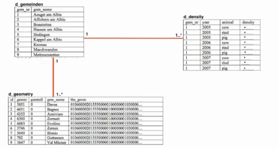
In this fort the minor subject Computer Science Lukas Urech created different additional tables to the Swiss Feed Database. (Urech, 2013) Two of the new created tables are mainly used for this work. One is called d_density and lists the density of cows, rinds and pigs in each community. The second one is called d_geometry and has stored the coordinates of the boundaries of all communities in Switzerland.

The ifi created the whole Swiss Feed Database and the framework of the webpage consisting the Google Maps API, in which the information of the tables can be illustrated in a more understanding way to the user.

(5)

Components

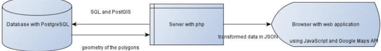
To visualize the animal density in the Swiss Feed Database three components are used. 1. A database with data of the animal density and administrative boundaries 2. Apache Server transforming with php http requests into SQL statements 3. User fronted composed of a web application running in a web browser

Figure 1: The three components

Database

The PostgeSQL database holding the data on animal density and the geodata itself is managed and administrated with pgadmin. Pgadmin is an open source product and provides a highly developed graphical user interface. (N.N., 2013)

In the database all the data which is used for the Swiss Feed Database is stored in different tables. For this work data of two of the tables are being used: d_density and d_geometry. Those two tables

are related over a third table d_gemeinden.

(6)

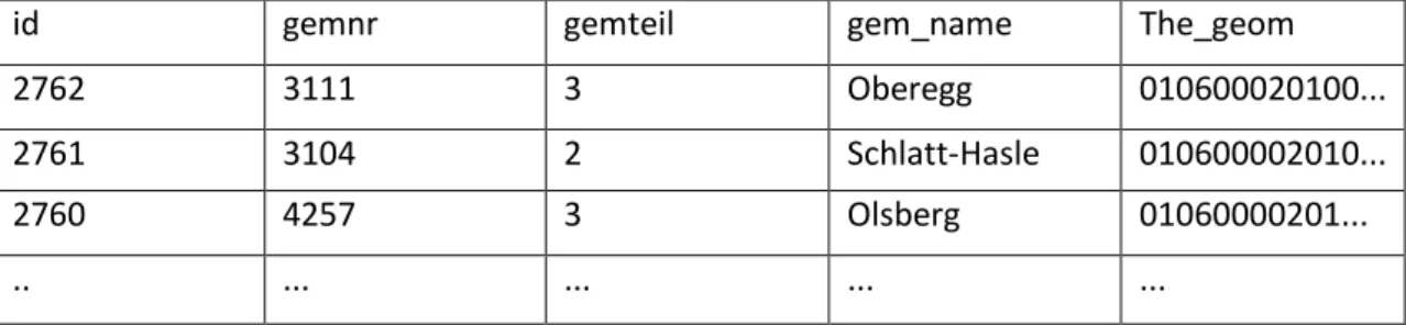
The table d_geometry has a column with a primary key id, a foreign key community number, information over enclaves of the community, the name and the geometry of the community. The field the_geom with the boundaries of the community is being used in further step to draw the features on the base map.

Table 1: g_geometry

id gemnr gemteil gem_name The_geom

2762 3111 3 Oberegg 010600020100...

2761 3104 2 Schlatt-Hasle 010600002010...

2760 4257 3 Olsberg 01060000201...

.. ... ... ... ...

The table d_density contains four columns: the gem_nr, which is the primary key, the year, the animal type and the density of that animal in the specific community and Year. These values are being used to visualize the animal density.

Table 2: d_density

gem_nr year animal density

3111 2005 cow 0.96

311 2005 pig 0.02

4257 2007 rind 0.82

.. ... ... ...

Server

Apache Tomcat is being used as web server. Apache is an open source framework to create web-based Java applications. (The apache software foundation, 2013)

The programming on the server is done with php. Php is a server based language, which can be embedded in html. It is suited for web development. (N.N., 2003) In this project php is being used to develop a CGI - script to handle the http requests from the web application turn them into SQL Queries respectively, afterwards the results from the queries is transformed into JSON documents that are processed by the web application of the Swiss Fed Database.

(7)

Browser

The user interacts with the web application over a frontend displayed in a browser. The application lets the user interact with the map: Different optional layers can be displayed and queried.

The web application uses the Google Maps API to render the features according the JSON document. Google maps API is a tool provided by Google to use different services with Google maps on your web application. In this project the AP is used to show spatial data on a Google base map.(Google, 2013) The language which is used to program the features in Google maps API s JavaScript. JavaScript is a dynamic programming language on the client side, often used for web applications, because it is easy to program and can handle different interfaces.

(8)

Visualizing administrative boundaries

The first step to visualize the animal density is to define and draw the shapes of the entities in which the density should be represented. Therefore, an interaction between the tree components has to be defined. The Server sends a query to the database to get the data out of it. The Server then

transforms this data in the right format, so that on the browser side it can be displayed and seen by the user.

Figure 3: The interactions between the tree components to draw polygons

1. Getting the data out of the database

As in the chapter Components explained that the language on the server side is php. With the help of php the data is taken out of the database. Php can use SQL and PostGIS statements to access the database. SQL is a data managing language and PostGIS is additional software, which provides functions to manage geographical data. (N.N., 2005)

To access the data from the, there is used a simple SQL-expression: SELECT the_geom

FROM d_geometry

WHERE the_geom is not null

2. The database sends the asked data

With the query above, one column with the geometry of the polygons of the communities is send back.

Table 3: Geometry dataset

The_geom

010600002015550000010000000103000.. 010600002015550000010000000103000.. ...

The information in the column the_geom is a hexadimensional number, which represents the coordinates of multiple polygons representing one community.

(9)

3. The server prepares the data to send to the browser side

The hexadimensional numbers representing the polygons of the communities are now at the server. Here they have to be prepared, so that they can be visualized on the web browser. This is done in tree steps.

a) The hexadimensional numbers have to be converted to text

b) The coordinates have to be transformed in the correct coordinate system c) The coordinates have be converted into the JSON format

To do this tree steps PostGIS provides tree function, which do those things for us.

a) The hexadimensional numbers have to be converted to a text file, so that in the next step the transformation can be done. The PostGIS function to do that step is ST_AsText().

In our case the data is a multpolygon and has following data structure:

MULTIPOLYGON(((555549 159921, 546017 148923, 544679 147056, …)))

b) Because the coordinates of the multipolygon are in the Swiss coordinate system, but Google maps in WGS 1984, they have to be transformed. This is done with the function ST_Transform().

The input to the function is the multipolygon text structure from a) and a specific code to do that transformation. In this case the code is 4326.

c) At last, the coordinates should be in a format, so that they can be compatible to JavaScript and therefore visualized with Google maps API in the web browser. The format which is used here is called JavaScript Object Notation (JSON) format. JSON is a simple programming language, which

is easy to read in many different languages and therefore used for data interchange. (“JSON,”

n.d.) To transform the query result into a response that can be used from the web application it has to be transformed into a valid JSON file. The function to do this step is ST_AsGeoJSON().

This function creates for every polygon a string which looks the following way:

{“polygon”: [[[x1, y1], [x2,y2],….]]}

For performance reasons it is not helpful to send a single JSON response for every single

geometry. Therefore, they are merged into one string, which later is also more efficient to use in JavaScript, where the data is further used. This is done with a for-loop like described in the code snippet below.

echo '({"polygons":[';

for ($i = 0; $i < $rows; $i++){ if ($i > 0) echo ',';

$row = pg_fetch_array($result, $i);

$mod_string = substr($row[0], strrpos($row[0],':') + 2);

$mod_string = substr($mod_string, 0, strlen($mod_string) - 2); echo $mod_string;

} echo ']})';

(10)

If all the three steps are combined, this leads to this php script: $query = pg_query("

SELECT st_asGeoJSON(st_astext(st_transform(the_geom, 4326))) FROM d_geometry

WHERE the_geom is not null");

$rows = pg_numrows($result); echo '({"polygons":[';

for ($i = 0; $i < $rows; $i++){ if ($i > 0) echo ',';

$row = pg_fetch_array($result, $i);

$mod_string = substr($row[0], strrpos($row[0],':') + 2);

$mod_string = substr($mod_string, 0, strlen($mod_string) - 2); echo $mod_string;

}

echo ']})';

The structure of the JSON string, which the browser side gets from the query above, is in the following structure:

{„polygons“:[[[x1-coord., y2-coord.],[x2-coord., y2-coord.],...,[xn-coord., yn-coord.]]]}

4. Drawing the polygons with JavaScript

The administrative boundaries are drawn onto the map using JavaScript. The data of the coordinates can be extracted from the JSON string which was in the previous step created in php.

var data = eval(httpObject.responseText);

for (var i = 0; i < data.polygons.length; i++){

var coords = new Array(data.polygons[i].length); for (var j = 0; j < data.polygons[i].length; j++){

coords[j] = new

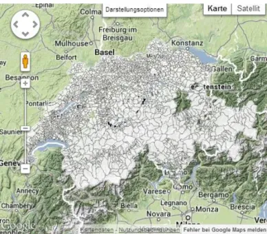
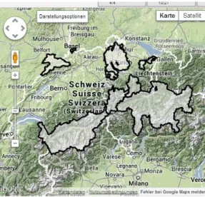
google.maps.LatLng(data.polygons[i][j][1],data.polygons[i][j][0]); In the screenshot of the output of this code all the communities of Switzerland are visualized.

(11)

Figure 4: Screenshot of the polygons representing the communities of Switzerland

5. Evaluation

The result as it is show above can now be optimized in different ways.

One problem which occurred is the visualizing of the multipolygons. Multipolygons are more difficult to visualize and therefore in this work converted to single Polygons. By converting the multipoygons to polygons data is lost. The goal is to keep this data loss as small as possible.

The user wants to see the visualization as fast as possible and therefore the data size which is sent from the server should be as small as possible.

For different scales the size of the boundaries should differ. If, for example, the user zooms to the

whole Switzerland, it’s not useful to see the boundaries of the communities, but rather of the

cantons. Multipolygons

Because the boundaries of the communities are not always single polygons, for example if they have an exclave or inclose another polygon, they are stored as multipolygons . Multipolygons are being created when several x, y coordinates describe more than one feature. This means that one entry in the field the geometry describes more than one feature. Multpolygons are more complicated to visualize and not subject of this work.

(12)

Figure 5: the canton St. Gallen and Appenzell as an example of polygon inclosing another polygon

To transform the multipolygons into polygons, there are several options. Two options provided by PostGIS are tested to the converting of the polygons: ST_ConvexHull() and ST_GeometryN(). The time needed to send the data from the server and the data size send are compared in figure 6 and 7.

Figure 6: Time needed to get the data from the server

Figure 7: Size of the data which gets send to the server

0 5 10 15 20 0 1000 2000 3000 tim e n e e d e d in se co n d s Number of polygons mit st_convexhull() mit geometryn(geom, 1) 0 5000 10000 15000 20000 25000 30000 35000 0 1000 2000 3000 d ta si ze in KB Number of boundaries mit st_convexhull() mit geometryn(geom,1)

(13)

Multipolygon to Polygon with the function ST_ConvexHull()

The principle of this function is to simplify the polygon by simplifying their shape. The shape is simplified by creating a convex geometry around all the features of the multipolygons.

The advantage of this function is that the data size is rather small, and therefore also the time needed to draw the polygons.

The disadvantage of this very simple generalization algorithm is the inaccuracy in terms of shape characteristics of the administrative units. The topology is destroyed and especially on small scale maps the cartographic representations of the polygons are useless.

Figure 8: Screenshot of the visualization with ST_ConvexHull()

Generalize a polygon using ST_GeometryN()

The principle of this function is that a 1-based single geometry is returned. The multipolygons are therefore transformed to one single polygon. Some of the vertices describing the feature area get lost, but not as much as with the function ST_ConvexHull(). Above all the natural shape of the polygon is maimed. Therefore the boundaries drawn with this function are very exact and the solution is cartographic appealing.

The disadvantage of this solution is that the data is still too big that the Google map API is able to render the features in a reasonable amount of time. Besides, those exact boundaries are not very useful for big scale map extents

(14)

Defining scale ranges to display different administrative units

In a smaller zoom level the boundary of the communities are hard to see. Therefore the communities should be aggregated, and the boundaries of the cantons should be shown. All the communities of one canton are merged and the outer boundary in then the boundary of the canton.

The function ST_Union() of Post-GIS can be used for that occasion.

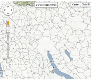
As you can see in the screenshot of the result of this union, not all the cantons are displayed. This is the same problem as described in the section Multipolygon. The cantons which are not displayed are multipolygons.

Figure 10: Screenshot of the merged communities to cantons

In a further step, there communities could also be merged to districts, so that there is one size between communities and cantons.

This method reduces the data size and time to draw the polygons for larger zoom levels and the map is better understandable for the user.

(15)

Visualizing the animal density

Now that the areas are visualized, they should be colored according to the density of the animals. The steps to do so are the same as described in the chapter Visualizing administrative boundaries, but the data and therefore the coding differs from this chapter.

Figure 11: The interactions between components to visualize the density

1. Getting the data out of the database

To get the density data out of the database, there has to be created an SQL-query, which shows the density of each animal per year and administrative unit. Because in the d_density table there is just the number and not the name of each community, the d_density and the d_geometry table need to be joined, so that we can see the density of each polygon.

SELECT d_geometry.gem_name, d_density.density, d_geometry.the_geom FROM d_density, d_geometry

WHERE d_density.gem_nr = d_geometry.gemnr

AND d_density.year ='2010' and d_density.animal='cow'

To simplify the process as an example, the query returns the density of the cows in 2010.

2. The database sends the asked data to the server

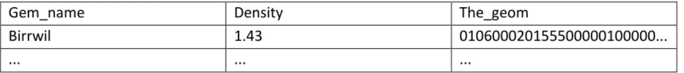
The queried result contains three columns containing the name of the community, the density of cows in 2010 and the geometry of the specific community.

Table 4: Table with communities, density and geometry

Gem_name Density The_geom

Birrwil 1.43 010600020155500000100000...

(16)

3. The server sends the data to the browser

The transformation of the density data to the JSON string is easier than with the polygons. The density has to be read by a for-loop out of the query result.

$density = '"density":['; for ($i = 0; $i < $rows; $i++){

if ($i > 0){

$density .= ','; }

$row = pg_fetch_array($result, $i); $density .= $row[2];

};

$density .= ']';

The existing string has just to be extended with the density information. echo '({';

echo $polygons; echo ',';

echo $density; echo '})';

The JSON-string, which can be created from this information is the following:

{„polygons“:[[[x1-coord., y2-coord.],[x2-coord., y2-coord.],...,[xn-coord.,

yn-coord.]]], „density“: cow_density}

4. Coloring the polygons according to their density

To color the choropleth map the livestock density is being used in a specific year. This density is defined as the number of animal per hectare. The coloring according to the density can be done in different ways. Either the density values can be grouped in different classes or the data can be normalized by defining the minimum and maximum value and coloring the values evenly between those two values.

Coloring by classes

To color the polygon by classes, the number and range of classes has to be defined. This can be done with a statistical program to analyze the data. In JavaScript classes can be defined with an if-cause. var co;

if (data.density[i]<1)co= 'rgb(0,255,0)';

else if (data.density[i]>1.0001&& data.density[i] <2)co = 'rgb(0,0,255)' ; else co ='rgb(255,0,0)';

var polygon = new google.maps.Polygon({

path: coords, fillColor: co,

(17)

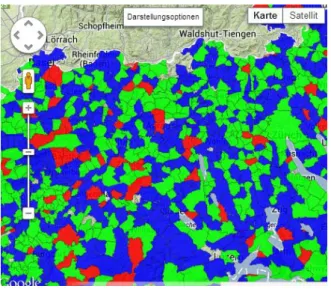
The advantage of this method is that outliers are not a big problem because they just belong to the highest class. But they classes have be defined for each dataset again, because the data never looks the same. In Figure 12 the cow density of 2010 is visualized by the code above. Red communities have a cow density over 2 cows per hectare, blue colored communities between 1 and 2 cows per hectare and green colored communities let than 1 cow per hectare.

Figure 12: Visualization of the cow density 2010 in tree classes

Coloring by normalization

A second way to visualize the density is by normalization. The coloring is done evenly distributed between the minimum and maximum density value of a dataset. The minimum and maximum value we extract with php from the dataset. At the beginning the minimum and maximum density value are set to -1. Afterwards the loop checks each value. If it is smaller than the minimum or larger than the maximum a new minimum or maximum is set.

for ($i = 0; $i < $rows; $i++){ if ($i > 0){

$density .= ','; $polygons .= ','; }

if ($min_density == -1){

if (isset($row[2])) $min_density = $row[2]; }else {

if (isset($row[2])){

if ($min_density > $row[2]) $min_density = $row[2]; }

}

if ($max_density == -1){

if (isset($row[2])) $max_density = $row[2]; }else {

if (isset($row[2])){

if ($max_density < $row[2]) $max_density = $row[2]; }

(18)

The minimum and maximum value is then sent in the JSON-string to the javascript-file in the same way also the polygons and density is sent, where the coloring is done with the following code.

var norm_density = 0.5;

if ((data.max_density - data.min_density) > 0){

norm_density = (data.density[i] - data.min_density)/(data.max_density - data.min_density);

}

var red = 0;

if (norm_density <= 0.5) red = 0;

else if (norm_density >= 0.75) red = 255;

else red = Math.round((norm_density-0.5)/0.25*255);

var green = 0;

if (norm_density >= 0.25 && norm_density <= 0.75) green = 255;

else if (norm_density < 0.25) green = Math.round(norm_density/0.25*255);

else green = Math.round((1-((norm_density-0.75)/0.25))*255);

var blue = 0;

if (norm_density <= 0.25) blue = 255;

else if (norm_density >= 0.5) blue = 0;

else blue = Math.round((1-((norm_density-0.25)/0.25))*255);

var polygon = new google.maps.Polygon({

path: coords,

strokeWeight: 0.25,

fillColor: "rgb(" + red + "," + green + "," + blue + ")",

fillOpacity: 0.85

}); polygon.setMap(map);

The advantage of this method is that once the script is defined, it can be used of every dataset. The disadvantage is that the classes are always different and if we look for example at the cow density of several years, the coloring represents not always the same density. Therefore a comparison is harder to do.

(19)

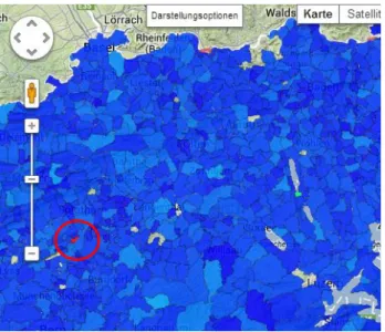
Figure 13: Visualization of the cow density 2010 with normalized values

In the screenshot above (Figure 13) most of the communities are in a bluish color because the values are close together comparing to an outliner in red. To correct this problem the outliners have to be removed and the normalization is just made for density values smaller than 4 cows/hectare. The result of this correction can be seen in Figure 14.

(20)

5. Evaluation

To evaluate which coloring method would be the best for the cow density in 2010 a histogram was crated.

Figure 15: Histogram of the animal density

The problem of the data is that most of it is between 0 and 4 cows/ha and just three values are above. If normalization is used those outliners would increase the range and the other values would all appear in one color. Therefore classing is the better solution, because the class can be defined with the help of the histogram. And the outliners would just be in the highest class. In conclusion it can be said that there are other ways to build classes. Among them there are some that respect outliers and also the fact, that most of the values are similar and therefore there is no big change in the choropleth map. For instance natural breaks analyses y Value gaps in the histogram. Where the y

– Value is the biggest, the class break is being set. Another way to have a nice color variation in the map is using quintiles. There a value has the same chance to fall into a class and therefore every class has the exact same amount of values.

animal/h a amo u n t

(21)

Result and further work

Goal of the work is an additional functional layer in the web application of the Swiss Feed Database. Users can display the layer and use it for further analysis together with existing ones.

The final result of the additional layer which the user can display in the web application of the Swiss Feed Database can be seen on the web page: www.feed-alp.admin.ch

On this web interface the user can now display by drop-down menu (1) different layers and overlay them onto the base map (2) and the animal density.

Figure 16: Screenshot of the result in the Swiss Feed database

This work shows that for rudimental requirements the above described components and workflows are sufficient. But the extend of this work was not big enough to solve all the problems occurring by visualizing the animal density in the map. There are several things which should be improved in further work.

As soon as there is more complex cartography involved or the amount of features to render onto the map are becoming bigger the architecture either reaches its limits or a lot of (CGI-) scripting is needed to create the rather complex generalization algorithms or creating Geo Queries that only queries data from a certain map extent assemble a high performance and yet cartographically appealing web application there is the possibility to server the map as a service. The under the open soure X/MIT license published UMN MapServer has the capabilities to host such services. WMS Services serve a picture file to the client whereas in a WFS Service the vector graphics are being served. The advantage of such service based architectures is, that the service one created can also be used by another piece of software for instance another web application or a smartphone application. Another improvements to do, is to develop a solution to visualize the multipolygons, so that there is no data lost by transforming them into polygons and that also enclaves and inclosed parts of

administrative regions can be displayed properly. 1

(22)

Finally, there could also being considered to create layers showing the change in animal density over time. So that region where there is a big change in the amount of animals can be detected and compared with other factors as changing in nutrition or ground properties.

(23)

References

admin.ch. (2013). Agroscope - Wir forschen für Sie! Retrieved September 19, 2013, from http://www.agroscope.admin.ch/aktuell/index.html?lang=de
Google. (2013). Google Maps API — Google Developers. Retrieved September 16, 2013, from https://developers.google.com/maps/?hl=de
ifi. (2013, May 21). The Swiss Feed Database. Retrieved August 26, 2013, from http://www.ifi.uzh.ch/dbtg/research/sfdb.html
N.N. (2013). PHP: Preface - Manual. Retrieved September 18, 2013, from http://www.php.net/manual/en/preface.php
N.N. (2005). PostGIS 2.0 Manual.
N.N. (2013). pgAdmin: PostgreSQL administration and management tools. Retrieved September 16, 2013, from http://www.pgadmin.org/
The apache software foundation. (2013). Welcome to The Apache Software Foundation! Retrieved September 16, 2013, from http://apache.org/
Urech, L. (2013). Embedding animal density information into the Swiss Feed Database (Facharbeit im Nebenfach Informatik). Universität Zürich, Zürich.