Modern statistics for spatial point processes
April 25, 2007
Jesper Møller and Rasmus P. Waagepetersen
Department of Mathematical Sciences, Aalborg University
Abstract: We summarize and discuss the current state of spatial point process theory and directions for future research, making an analogy with generalized linear models and random effect models, and illustrating the theory with various examples of applications. In particular, we consider Poisson, Gibbs, and Cox process models, diagnostic tools and model checking, Markov chain Monte Carlo algorithms, computational methods for likelihood-based inference, and quick non-likelihood approaches to inference.
Keywords: Bayesian inference, conditional intensity, Cox process, Gibbs point process, Markov chain Monte Carlo, maximum likelihood, perfect simulation, Poisson process, residuals, simulation free estimation, summary statistics.
1
Introduction
Spatial point pattern data occur frequently in a wide variety of scientific disci-plines, including seismology, ecology, forestry, geography, spatial epidemiology, and material science, see e.g. Stoyan & Stoyan (1998), Kerscher (2000), Boots, Okabe & Thomas (2003), Diggle (2003), and Ballani (2006). The classical spa-tial point process textbooks (Ripley, 1981, 1988; Diggle, 1983; Stoyan, Kendall & Mecke, 1995; Stoyan & Stoyan, 1995) usually deal with relatively small point patterns, where the assumption of stationarity is central and non-parametric methods based on summary statistics play a major role. In recent years, fast computers and advances in computational statistics, particularly Markov chain
Monte Carlo (MCMC) methods, have had a major impact on the develop-ment of statistics for spatial point processes. The focus has now changed to likelihood-based inference for flexible parametric models, often depending on covariates, and liberated from restrictive assumptions of stationarity. In short, ‘Modern statistics for spatial point processes’, where recent textbooks include Van Lieshout (2000), Diggle (2003), Møller & Waagepetersen (2003b), and Bad-deley, Gregori, Mateu, Stoica & Stoyan (2006).
Much of the literature on spatial point processes is fairly technical with ex-tensive use of measure theoretical terminology and statistical physics parlance. This has made the theory seem rather difficult. Moreover, in connection with likelihood-based inference, many statisticians may be unfamiliar with the con-cept of defining a density with respect to a Poisson process. It is our intention in Sections 3–9 to give a concise and non-technical introduction to the modern theory, making analogies with generalized linear models and random effect mod-els, and illustrating the theory with various examples of applications introduced in Section 2. In particular, we discuss Poisson, Gibbs, and Cox process mod-els, diagnostic tools and model checking, MCMC algorithms and computational methods for likelihood-based inference, and quick non-likelihood approaches to inference. Section 10 summarizes the current state of spatial point process the-ory and discusses directions for future research.
For definiteness, we mostly work with point processes defined in the plane R2, but most ideas easily extend to the general case of Rd or more abstract spaces. For ease of exposition, no measure theoretical details are given; see instead Møller & Waagepetersen (2003b) and the references therein. The com-putations for the data examples were done using theRpackagespatstat (Bad-deley & Turner, 2005, 2006) or our own programmes inCandR, where the code is available at www.math.aau.dk/~rw/sppcode. Since we shall often refer to our own monograph, please notice the comments and corrections to Møller & Waagepetersen (2003b) atwww.math.aau.dk/~jm.
2
Data examples
The following four examples of spatial point pattern data are from plant and animal ecology, and are considered for illustrative purposes in subsequent sec-tions. In each example, theobservation windowrefers to the area where points of the pattern can possibly be observed, i.e. when the point pattern is viewed
as a realization of a spatial point process (Section 3.1). Absence of points in a region, where they could potentially occur, is a source of information comple-mentary to the data on where points actually did occur. The specification of the observation window is therefore an integral part of a spatial point pattern data set.
Figure 1 shows positions of 55 minke whales (Balaneoptera acutorostrata) observed in a part of the North Atlantic near Spitzbergen. The whales are observed visually from a ship sailing along predetermined so-called transect lines. The point pattern can be thought of as an incomplete observation of all the whale positions, since it is only possible to observe whales within the vicinity of the ship. Moreover, whales within sighting distance may fail to be observed due to bad weather conditions or if they are diving. The probability of observing a whale is a decreasing function of the distance from the whale to the ship and is effectively zero for distances larger than 2 km. The observation window is therefore a union of narrow strips of width 4 km around the transect lines. The data in Figure 1 do not reflect the fact that the whales move and that the whales are observed at different points in time. However, the observations from different transect lines may be considered approximately independent due to the large spatial separation between the transect lines. More details on the data set and analysis of line transect data can be found in Skaug, Øien, Schweder & Bøthun (2004), Waagepetersen & Schweder (2006), and Buckland, Anderson, Burnham, Laake, Borchers, and Thomas (2004). The objective is to estimate the abundance of the whales, or equivalently the whale intensity. The whales tend to cluster around locations of high prey intensity, and a point process model for all whale positions (including those not observed) should take this into account. The point process model used in Waagepetersen & Schweder (2006) is described in Example 4.2 and analyzed in Examples 7.3 and 7.4.
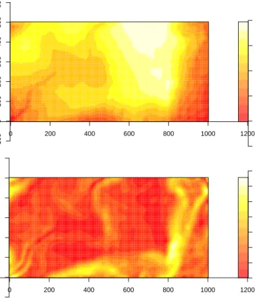
In studies of biodiversity of tropical rain forests, it is of interest to study whether the spatial patterns of the many different tree species can be related to spatial variations in environmental variables concerning topography and soil properties. Figure 2 shows positions of 3605Beilschmiedia pendula Lauraceae trees in the tropical rain forest of Barro Colorado Island. This data set is a part of a much larger data set containing positions of hundreds of thousands of trees belonging to hundreds of species, see Hubbell & Foster (1983), Condit, Hubbell & Foster (1996), and Condit (1998). In addition to the tree positions, covariate information on altitude and norm of altitude gradient is available, see Figure 3. Phrased in point process terminology, the question is whether the intensity of
Figure 1: Observed whales along transect lines. The enclosing rectangle is of dimensions 263 km by 116 km.
Beilschmiediatrees may be viewed as a spatially varying function of the covari-ates. In the study of this question, it is, as for the whales, important to take into account clustering, which in the present case may be due to tree reproduction by seed dispersal and possibly unobserved covariates. Different point process models for the tree positions are introduced in Examples 4.1 and 4.3 and further considered in Figure 9 and Examples 7.5, 8.1, 8.3, and 8.4.
Figure 2: Locations ofBeilschmiedia pendula Lauraceaetrees observed in a 1000 m by 500 m rectangular window.
Another pertinent question in plant ecology is how trees interact due to competition. Figure 4 shows positions and stem diameters of 134 Norwegian spruces. This data set was collected in Tharandter Forest, Germany, by the forester G. Klier and was first analyzed using point process methods by Fiksel (1984). The data set is an example of a marked point pattern, with points given by the tree locations and marks by the stem diameters. The discs in Figure 4 are of radii five times the stem diameters and may be thought of as
0 200 400 600 800 1000 1200 −100 0 100 200 300 400 500 600 110 120 130 140 150 160 0 200 400 600 800 1000 1200 −100 0 100 200 300 400 500 600 0 0.05 0.15 0.25 0.35
Figure 3: Altitude (upper plot) in meter and norm of altitude gradient (lower plot).
‘influence zones’ of the trees, see Penttinen, Stoyan & Henttonen (1992) and Goulard, S¨arkk¨a & Grabarnik (1996). The regularity in the point pattern is to a large extent due to forest management. From an ecological point of view it is of interest to study how neighbouring trees interact, i.e. when their influence zones overlap. It is then natural to model the conditional intensity, which roughly speaking determines the probability of observing a tree at a given location and of given stem diameter conditional on the neighbouring trees. In Example 5.1, we consider a simple model where the conditional intensity depends on the amount of overlap between the influence zones of a tree and its neighbouring trees. The spruces are also considered in Figure 10 and Example 7.1.
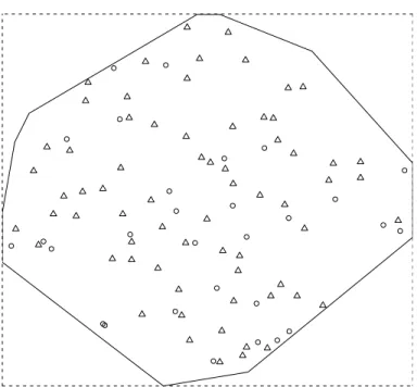
Our last data set is an example of a multitype point pattern, with two types of points specifying the positions of nests for two types of ants, Messor was-manniandCataglyphis bicolor, see Figure 5 and Harkness & Isham (1983). Note
. . . . .. . . . . . . . . . . . . . . . . . . . . . . . . . . . . . . . . . . . . . . . . . . . . . . . . . . . . . . . . . . . . . . . . . . . . . . . . . . . . . . . . . . . . . . . . . . . . . . . . . . . . . . . . . . . . . . . . .. . . . . . . . . . . . . . .
Figure 4: Norwegian spruces observed in a rectangular 56 m by 38 m window. The radii of the discs equal 5 times the stem diameters.
the rather atypical shape of the observation window. The interaction between the two types of ants is of main interest for this data set. Biological knowl-edge suggests that theMessorants are not influenced by presence or absence of Cataglyphisants when choosing sites for their nests. TheCatagplyphisants, on the other hand, feed on deadMessorsand hence the positions of Messor nests might affect the choice of sites forCataglyphis nests. H¨ogmander and S¨arkk¨a (1999) therefore specify a hierarchical model: first a model for the conditional intensity of aMessornest at a particular location given the neighbouringMessor nests, and second a conditional intensity for aCataglyphisnest given the neigh-bouring Cataglyphisnestsand the neighbouringMessor nests. Further details are given in Example 5.2, Figures 7–8, and Examples 7.2 and 8.2.
These examples illustrate many important features of interest for spatial point process analysis: clusteringdue to e.g. seed dispersal or unobserved vari-ation in prey intensity (as for the tropical rain forest trees and the whales), inhomogeneity e.g. caused by a thinning mechanism or covariates (as for the whales and tropical rain forest trees), and interaction between points, where the interaction possibly depends on marks associated with the points (as for the Norwegian spruces). The examples also illustrate different types of observation windows.
Figure 5: Locations of nests for Messor (triangles) and Cataglyphis (circles) ants. Enclosing rectangle for observation window is 414.5 ft by 383 ft.
3
Preliminaries
3.1
Spatial point processes
In the simplest case, aspatial point processXis afinite random subsetof a given bounded region S ⊂ R2, and a realization of such a process is a spatial point patternx={x1, . . . , xn} ofn≥0 points contained in S. We say that thepoint
process is defined onS, and we write x =∅ for the empty point pattern. To specify the distribution ofX, one may specify the distribution of the number of points,n(X), and for eachn≥1, conditional onn(X) =n, the joint distribution of thenpoints in X. An equivalent approach is to specify the distribution of the variablesN(B) =n(XB) for subsetsB⊆S, whereXB =X∩B.
If it is not known on which region the point process is defined, or if the process extends over a very large region, or if certain invariance assumptions such as stationarity are imposed, then it may be appropriate to consider an infinite point process onR2. We define aspatial point processXon R2 as a lo-cally finite random subset ofR2, i.e.N(B) is a finite random variable whenever
its distribution is invariant under translations inR2 respective rotations about the origin inR2. Stationarity and isotropy may be reasonable assumptions for point processes observed within a homogeneous environment. These assump-tions appeared commonly in the older point process literature, where typically rather small study regions were considered. We shall abandon them when spatial covariate information is available.
In most applications, the observation window W (see Section 2) is strictly contained in the regionS, where the point process is defined. SinceX\W is unobserved, we face a missing data problem, which in the spatial point process literature is referred to as a problem ofedge effects.
3.2
Moments
The mean structure of the count variables N(B), B ⊆R2, is summarized by themoment measure
µ(B) = EN(B), B ⊆R2. (1) In practice the mean structure is modelled in terms of a non-negativeintensity functionρ, i.e.
µ(B) =
Z
B
ρ(u) du
where we may interpretρ(u) duas the probability that precisely one point falls in an infinitesimally small region containing the locationuand of area du.
The covariance structure of the count variables is most conveniently given in terms of thesecond order factorial moment measure µ(2). This is defined by
µ(2)(A) = E 6 = X u,v∈X 1[(u, v)∈A], A⊆R2×R2, (2)
where 6= over the summation sign means that the sum runs over all pairwise different pointsu, vinX, and1[·] is the indicator function. For bounded regions
B⊆R2 andC⊆R2,
Cov[N(B), N(C)] =µ(2)(B
×C) +µ(B∩C)−µ(B)µ(C).
second order product densityρ(2), µ(2)(A) =Z 1[(u, v)
∈A]ρ(2)(u, v) dudv
whereρ(2)(u, v)dudvmay be interpreted as the probability of observing a point
in each of two regions of infinitesimally small areas duand dv and containing
uand v. More generally, for integers n ≥ 1, the nth order factorial moment measureµ(n) is defined by µ(n)(A) = E 6 = X u1,...,un∈X 1[(u1, . . . , un)∈A], A⊆R2n, (3)
with correspondingnth order product density ρ(n). From (3) we obtain
Camp-bell’s theorem E 6 = X u1,...,un∈X h(u1, . . . , un) = Z h(u1, . . . , un)ρ(n)(u1, . . . , un) du1,· · ·dun (4)
for non-negative functionsh. The nth order moment measure is given by the right hand side of (3) without6=. The reason for preferring the factorial moment measures are the nicer expressions for the product densities, cf. (6) and (16).
In order to characterize the tendency of points to attract or repel each other, while adjusting for the effect of a large or small intensity function, it is useful to consider thepair correlation function
g(u, v) =ρ(2)(u, v)/(ρ(u)ρ(v)) (5) (providedρ(u)>0 andρ(v)>0). If points appear independently of each other,
ρ(2)(u, v) = ρ(u)ρ(v) and g(u, v) = 1 (see also (6)). When g(u, v) >1 we
in-terpret this as attraction between points of the process at locations u and v, while ifg(u, v)<1 we haverepulsionat the two locations. Translation invari-anceg(u, v) =g(u−v) ofgimplies thatXissecond order intensity reweighted stationary(Baddeley, Møller & Waagepetersen, 2000 and Section 6.2.1), and in applications it is often assumed thatg(u, v) =g(ku−vk), i.e. that g depends only on the distanceku−vk. Notice that very different point process models can share the sameg function (Baddeley & Silverman, 1984, Baddeley et al., 2000, Diggle, 2003 (Section 5.8.3)).
-thinning of X is obtained by independently retaining each point u in X with probabilityπ(u). It follows easily from (4) thatπ(u1)· · ·π(un)ρ(n)(u1, . . . , un)
is thenth order product density of the thinned process. In particular,π(u)ρ(u) is the intensity function of the thinned process, whilegis the same for the two processes.
3.3
Marked point processes
In addition to each point u in a spatial point process X, we may have an associated random variable mu called a mark. The mark often carries some
information about the point, for example the radius of a disc as in Figure 4, the type of ants as in Figure 5, or another point process (e.g. the clusters in a shot noise Cox process, see Section 4.2.2). The processΦ ={(u, mu) :u ∈ X} is
called amarked point process, and indeed marked point processes are important for many applications, see Stoyan & Stoyan (1995), Stoyan & W¨alder (2000), Schlather, Riberio & Diggle (2004), Schlather (2001), Møller & Waagepetersen (2003b). For the models presented later in this paper, the marked point process model of discs in Figure 4 will be viewed as a point process inR2×(0,∞), and the bivariate point process model of ants nests in Figure 5 will be specified by a hierarchical model so that no methodology specific to marked point processes is needed.
3.4
Generic notation
Unless otherwise stated,
Xdenotes a generic spatial point process defined on a regionS⊆R2;
W ⊆S is a bounded observation window;
x={x1, . . . , xn} is either a generic finite point configuration or a realization
ofXW (the meaning ofxwill always be clear from the context);
z(u) = (z1(u), . . . , zk(u)) is a vector of covariates depending on locationsu∈
S such as spatially varying environmental variables, known functions of the spatial coordinates themselves or distances to known environmental features, cf. Berman & Turner (1992) and Rathbun (1996);
β= (β1, . . . , βk) is a corresponding regression parameter;
4
Modelling the intensity function
This section discusses spatial point process models specified by a determinis-tic or random intensity function by analogy with generalized linear models and random effects models. Particularly, two important model classes, namely Pois-son and Cox/cluster point processes are introduced. Roughly speaking, the two classes provide models for no interaction and aggregated point patterns, respectively.
4.1
The Poisson process
APoisson processX defined onS and with intensity measureµ and intensity functionρsatisfies for any bounded regionB⊆S withµ(B)>0,
(i) N(B) is Poisson distributed with meanµ(B),
(ii) conditional onN(B), the points inXB are i.i.d. with density proportional
toρ(u),u∈B.
Poisson processes are studied in detail in Kingman (1993). They play a funda-mental role as a reference process for exploratory and diagnostic tools and when more advanced spatial point process models are constructed.
Ifρ(u) is constant for allu∈S, we say that the Poisson process is homoge-neous. Realizations of the process may appear to be rather chaotic with large empty space and close pairs of points, even when the process is homogeneous. The Poisson process is a model for ‘no interaction’ or ‘complete spatial ran-domness’, since XA andXB are independent whenever A, B ⊂S are disjoint.
Moreover,
ρ(n)(u1, . . . , un) =ρ(u1)· · ·ρ(un), g≡1, (6)
reflecting the lack of interaction. Stationarity means thatρ(u) is constant, and implies isotropy ofX. Note that another Poisson process results if we make an independent thinning of a Poisson process.
Typically, a log linear model of the intensity function is considered (Cox, 1972),
logρ(u) =z(u)βT. (7)
The independence properties of a Poisson process are usually not realistic for real data. Despite of this the Poisson process has enjoyed much popularity due to its mathematical tractability.
4.2
Cox processes
One natural extension of the Poisson process is aCox processXdriven by a non-negative process Λ = (Λ(u))u∈S, such that conditional on Λ, X is a Poisson
process with intensity function Λ (Cox, 1955; Mat´ern, 1971; Grandell, 1976; Daley & Vere-Jones, 2003).
Three points of statistical importance should be noticed. First, though Λ
may be modelling a random environmental heterogeneity, X is stationary if
Λ is stationary. Second, we cannot distinguish the Cox process X from its corresponding Poisson processX|Λwhen only one realization ofXW is available,
cf. Møller & Waagepetersen (2003b, Section 5.1). Third, the likelihood is in general unknown, while product densities may be tractable. The consequences of the latter point are discussed in Sections 7 and 8.
4.2.1 Log Gaussian Cox processes
In analogy with random effect models, as an extension of the log linear model (7), take
log Λ(u) =z(u)βT+ Ψ(u) (8)
where Ψ = (Ψ(u))u∈S is a zero-mean Gaussian process. Then we call X a
log Gaussian Cox process (Møller, Syversveen & Waagepetersen, 1998). The covariance functionc(u, v) = Cov[Ψ(u),Ψ(v)] typically depends on some lower-dimensional parameter, see e.g. Example 4.1 below. To ensure local integrability of Λ(u), the covariance function has to satisfy certain mild conditions, which are satisfied for models used in practice.
The product densities are particularly tractable. The intensity function logρ(u) =z(u)βT+c(u, u)/2 (9) is log linear,g andc are in a one-to-one correspondence as
g(u, v) = exp(c(u, v))
and higher-order product densities are nicely expressed in terms of ρ and g
(Mølleret al., 1998). Another advantageous property is that we have no problem with edge effects, since XW is specified by the Gaussian process restricted to
W.
For the tropical rain forest trees in Figure 2, we consider in Example 7.5 infer-ence for a log Gaussian Cox process withz(u) = (1, z2(u), z3(u)), wherez2(u)
and z3(u) denote the altitude and gradient covariates given in Figure 3. An
exponential covariance functionc(u, v) = σ2exp(
−ku−vk/α) is used for the Gaussian process, whereσandαare positive parameters.
4.2.2 Shot noise Cox processes
Ashot noise Cox processXhas random intensity function Λ(u) = X
(c,γ)∈Φ
γk(c, u) (10)
where c ∈ R2, γ > 0, Φ is a Poisson process on R2×(0,∞), and k(c,·) is a density for a two-dimensional continuous random variable (Møller, 2003). Note that X is distributed as the superposition (i.e. union) of independent Poisson processesX(c,γ) with intensity functionsγk(c,·), (c, γ)∈Φ, where we interpret
X(c,γ) as a cluster with centre c and mean number of pointsγ. ThusX is an
example of a Poisson cluster process (Bartlett, 1964), and provides a natural model for seed setting mechanisms causing clustering, see e.g. Brix & Chadoeuf (2002). Simple formulae for the intensity and pair correlation functions of a shot noise Cox process are provided in Møller (2003).
Example 4.2. (Shot noise Cox process for minke whales) In Waagepetersen & Schweder (2006), the positions of minke whales in Figure 1 are modelled as an independent thinning of a shot noise Cox process. Lettingp(u) denote the probability of observing a whale at locationu, the process of observed whales is a Cox process driven by Λ(u) =p(u)P
(c,γ)∈Φγk(c, u). The cluster centres are assumed to form a stationary Poisson process with intensityκ, thec’s are independent of the γ’s, and the γ’s are i.i.d. gamma random variables with meanαand unit scale parameter. To handle edge effects,k(c,·) is the density ofN2(c, ω2I) restricted toc+ [−3ω,3ω]2.
A particular simple case of a shot noise Cox process is aNeyman-Scott process
X, where the centre points form a stationary Poisson process with intensityκ
and the γ’s are all equal to a positive parameter α(Neyman & Scott, 1958). If furthermorek(c,·) is a bivariate normal density with meanc and covariance matrixω2I, thenXis a(modified) Thomas process(Thomas, 1949). A
also isotropic with
g(r) = 1 + exp −r2/(4ω2)
/(4πκω2), r >0. (11)
Shot noise Cox process can be extended in various interesting ways by al-lowing the kernelkto depend on a random band-widthband replacingΦby a Poisson or non-Poisson process model for the points (c, γ, b) (Møller & Torrisi, 2005). In this paper, we consider instead an extension which incorporates co-variate information in a multiplicative way, i.e. an inhomogeneous Cox process driven by
Λ(u) = exp z(u)βT X (c,γ)∈Φ
γk(c, u) (12)
(Waagepetersen, 2007). A nice feature is that the pair correlation function of
Xis the same for (10) and (12), i.e. it does not depend on the parameterβ. Example 4.3. (Inhomogeneous Thomas model for tropical rain forest trees) In addition to the log Gaussian Cox process model for the tropical trees (Exam-ple 4.1), we consider an inhomogeneous Thomas process of the form (12),
Λ(u) = α
2πω2exp (β2z2(u) +β3z3(u)) X
c∈Φ
exp −ku−ck2/(2ω2)
where nowΦ denotes a stationary Poisson process with intensityκ. Then the intensity function is
ρ(u) =καexp (β2z2(u) +β3z3(u)) (13)
while the pair correlation function is equal to (11).
5
Modelling the conditional intensity function
Gibbs point processes arose in statistical physics as models for interacting parti-cle systems. The intensity function for a Gibbs process is unknown; instead, the Papangelou conditional intensityλ(u,x) (Papangelou, 1974) becomes the appro-priate starting point for modelling. The definition and interpretation ofλ(u,x) are given in Section 5.2 in terms of the density of a finite point process and in Section 5.4 using a more technical account for infinite point processes. The den-sity of a Gibbs point process is specified in Section 5.3. Though the denden-sity has an unknown normalizing constant, likelihood inference based on MCMC
meth-ods is easier for parametric Gibbs point process models than for Cox processes; see Section 7. While Cox processes provide flexible models for aggregation or clustering in a point pattern, Gibbs point processes provide flexible models for regularity or repulsion (Sections 5.3 and 10.3).
5.1
Finite point processes with a density
Throughout this section we assume thatS is bounded and Xis a finite point process defined on S. Moreover, Yρ denotes a Poisson process on S with
in-tensity measure µ and intensity functionρ. In particular, Y1 is theunit rate
Poisson process onS with intensity ρ ≡1. Before defining what is meant by the density ofX, we need the following useful Poisson expansion. IfF denotes any event of spatial point patterns contained inS, by (i)-(ii) in Section 4.1,
P(Yρ∈F) = ∞ X n=0 e−µ(S) n! Z Sn 1[x∈F]ρ(x1)· · ·ρ(xn) dx1· · ·dxn (14) wherex={x1, . . . , xn}.
By (14),Xhasdensityf with respect toY1 if
P(X∈F) = E [1[Y1∈F]f(Y1)] = ∞ X n=0 e−|S| n! Z Sn 1[x∈F]f(x) dx1· · ·dxn (15)
where|S|is the area ofS. Combining (3) and (15) it follows that
ρ(n)(u1, . . . , un) = Ef(Y1∪ {u1, . . . , un}) (16)
for anyn∈Nand pairwise different points u1, . . . , un ∈S. Conversely, under mild conditions,f can be expressed in terms of the product densitiesρ(n)
(Mac-chi, 1975). Furthermore, conditional onn(X) =nwith n≥1, thenpoints in
Xhave a symmetric joint density
fn(x1, . . . , xn)∝f({x1, . . . , xn}) (17)
onSn.
Apart from the Poisson process and a few other simple models such as the mixed Poisson process (Grandell, 1997), the density is not expressible in closed
form. For the Poisson processYρ, (14) gives f(x) = e|S|−µ(S) n Y i=1 ρ(xi). (18)
Thus, for a Cox process driven byΛ= (Λ(u))u∈S,
f(x) = E " exp |S| − Z S Λ(u) du Y u∈X Λ(u) # (19)
which in general is not expressible in closed form.
5.2
The conditional intensity
The usual conditional intensity of a one-dimensional point process does not ex-tend to two-dimensional point processes because of the lack of a natural ordering in R2. Instead, the Papangelou conditional intensity becomes the appropriate counterpart (Papangelou, 1974); a formal definition is given below.
Let the situation be as in Section 5.1, and suppose thatf ishereditary, i.e.
f(x)>0 andy⊂x ⇒ f(y)>0 (20) for finite point configurations x ⊂ S. This condition is usually assumed in practice.
Now, for locations u∈S and finite point configurationsx⊂S, the Papan-gelou conditional intensity is defined by
λ(u,x) =f(x∪ {u})/f(x\ {u}) (21) iff(x\ {u})>0, and λ(u,x) = 0 otherwise. The precise definition of λ(u,x) whenu∈xis not that important, and (21) just covers this case for completeness. Note thatλ(u,x) =λ(u,x\ {u}), and (20) implies thatf andλ are in a one-to-one correspondence.
For a Poisson process, the Papangelou conditional intensity is simply the intensity: iff(x)>0 is given by (18), thenλ(u,x) =ρ(u) does not depend on
x, again showing the absence of interaction in a Poisson process. Combining (16) and (20)–(21),
Recall that the conditional probability P(A|x) of an event A given X = x
satisfies P(A) = E[P(A|X)]. Thus due to the infinitesimal interpretation of
ρ(u) du(Section 3.2), it follows from (22) thatλ(u,x) dumay be interpreted as the conditional probability that there is a point of the process in an infinitesimal region containing u and of area du given that the rest of the point process coincides withx.
Often a densityf is specified by anunnormalized densityh, i.e.f ∝hwhere
his an hereditary function, for which the normalizing constant Eh(Y1) is well
defined but unknown. However,
λ(u,x) =h(x∪ {u})/h(x\ {u})
does not depend on the normalizing constant. This is one reason why inference and simulation procedures are often based on the conditional intensity rather than the density of the point process.
In practically all cases of spatial point process models, an unnormalized densityhislocally stable, that is, there is a constantK such that
h(x∪ {u})≤Kh(x) (23)
for allu∈S and finite x⊂S. Local stability implies both thathis hereditary and integrable with respect the to unit rate Poisson process. Local stability also plays a fundamental role when studying stability properties of MCMC algorithms (Section 9.2).
5.3
Finite Gibbs point processes
Consider again a finite point process Xdefined on the bounded region S and with hereditary densityf. This is aGibbs point process(also called a canonical ensemble in statistical physics) if
logλ(u,x) =X y⊆x
U(y∪ {u}) whenf(x)>0 (24)
where the function U(x) ∈ [−∞,∞) is defined for all non-empty finite point configurationsx⊂S, and we set log 0 =−∞. In statistical mechanical terms,
U is a potential.
A large selection of Gibbs point process models are given in Van Lieshout (2000) and Møller & Waagepetersen (2003b). Usually, a log linear model is
considered, where the first order potential is either constant or depends on spatial covariates
U(u)≡U({u}) =z(u)βT
and higher order potentials are of the form
U(x) =V(x)ψT
n(x), n(x)≥2
where theψn are so-called interaction parameters. Thenλis parameterized by
θ= (β, ψ2, ψ3, . . .) and is on log linear form
logλθ(u,x) = (t(x∪ {u})−t(x))θT (25) where t(x) = X u∈x z(u), X y⊆x:n(y)=2 V(y), X y⊆x:n(y)=3 V(y), . . . . (26)
Combining (21) and (24), the Gibbs process has density
f(x)∝exp X ∅6=y⊆x U(y) (27)
defining exp(−∞) = 0. Unless X is Poisson, i.e. when U(y) = 0 whenever
n(y) ≥ 2, the normalizing constant of the density is unknown. Usually for models used in practice, U(y) ≤ 0 if n(y) ≥ 2, which implies local stability (and hence integrability). This means that the points in the process repel one other, so that realizations of the process tend to be more regular than for a Poisson process. Most Gibbs models are pairwise interaction processes, i.e.
U(y) = 0 whenevern(y)≥3, and typically the second order potential depends on distance only,U({u, v}) =U(ku−vk). A hard core processwith hard core
r >0 hasU({u, v}) =−∞wheneverku−vk< r.
TheHammersley-Clifford theoremfor Markov random fields was modified to the case of spatial point processes by Ripley & Kelly (1977), stating that any hereditary density is of the form (27) and the following properties (I) and (II) are equivalent.
(I) U(x) = 0 whenever there exist two points{u, v} ⊆xsuch thatku−vk> R.
Hereb(u, R) is the closed disc with centreuand radius R. When (I) or (II) is satisfied,X is said to beMarkov withinteraction radius R, or more precisely, Markov with respect to the R-close neighbourhood relation. This definition and the Hammersley-Clifford theorem can be extended to an arbitrary sym-metric relation onS (Ripley & Kelly, 1977) or even a relation which depends on realizations of the point process (Baddeley & Møller, 1989). Markov point processes constitute a particular important subclass of Gibbs point processes, since the local Markov property (II) very much simplifies the computation of the Papangelou conditional intensity in relation to parameter estimation and simulation.
The property (I) implies a spatial Markov property. If B ⊂ S and ∂B =
{u6∈B :b(u, R)∩B 6=∅} is itsR-close neighbourhood, then the process XB
conditional onXBcdepends only onXBcthroughX∂B. The conditional process
XB|X∂B =x∂B is also Gibbs, with density
fB(xB|x∂B)∝exp X ∅6=y⊆xB U(y∪x∂B) (28)
where the normalizing constant depends onx∂B (the conditional density may
be arbitrarily defined if U(y) =−∞ for some non-empty point configuration
y⊆x∂B). The corresponding Papangelou conditional intensity is
λ(u,xB|x∂B) =λ(u,xB∪x∂B), u∈B. (29)
Example 5.1. (Overlap interaction model for Norwegian spruces) The condi-tional intensity for a Norwegian spruce with a certain influence zone should depend not only on the positions but also on the influence zones of the neigh-bouring trees, see Figure 4. A tree with influence zone given by the discb(u, mu),
whereuis the spatial location of the tree andmuis the influence zone radius, is
treated as a point (u, mu) inR3. Confining ourselves to a pairwise interaction
process, we define the pairwise potential by
U({(u, mu),(v, mv)}) =ψ|b(u, mu)∩b(v, mv)|, ψ≤0.
Hence, the strength of the repulsion between two trees (u, mu) and (v, mv) is
given by ψ times the area of overlap between the influence zones of the two trees. We assume that the influence zone radii belong to a bounded interval
M = [a, b], whereaandb are estimated by the minimal and maximal observed influence zone radii. We divide M into six disjoint subintervals of equal size, and define the first order potential by
U({(u, mu)}) =β(mu) =βk ifmu falls in thekth subinterval
where βk is a real parameter. This enables modelling the varying numbers
of trees in the six different size classes. However, the interpretation of the conditional intensity λθ((u, mu),x) = exp β(mu) +ψ X (v,mv)∈x |b(u, mu)∩b(v, mv)| (30)
is not straightforward — it is for instance not in general a monotone function of mu. On the other hand, for a fixed (u, mu), the conditional intensity will
always decrease if the neighbouring influence zones increase.
Example 5.2. (Hierarchical model for ants nests) The hierarchical model in H¨ogmander & S¨arkk¨a (1999) for the positions of ants nests is based on so-called Strauss processes with hard coresas described below.
For distancest >0, define
V(t;r) = −∞ ift≤r 1 ifr < t≤R 0 otherwise
whereRis the interaction range andr≥0 denotes a hard core distance (or no hard core ifr= 0). For the Messor nests, the Strauss process with hard core
rM is given by first and second order potentials
UM1({u}) =βM, UM2({u, v}) =ψMV(ku−vk;rM),
and no higher order interactions. The conditional intensity for a putative nest at a location uis thus zero if an existing nest occur within distance rM from
u, and otherwise the log conditional density is given by the sum ofβM andψM
times the number of neighbouring nests within distanceR. Given the pattern
xM of Messor nests, the Cataglyphisnests are modelled as an inhomogeneous
corerC between theCataglyphisnests, i.e. using potentials
UC1({u}) =βC+ψCM
X
v∈xM
V(ku−vk;rCM), UC2({u, v}) =ψCV(ku−vk;rC).
Finally, the hard cores are estimated by the observed minimum interpoint dis-tances, which are biased maximum likelihood estimates.
Using positive hard coresrM andrC may be viewed as an ad hoc approach
to obtain a model which is well-defined for all real values of the parameters
βM, βC, ψM,ψCM, andψC, whereby both repulsive and attractive interaction
within and between the two types of ants can be modelled. However, as noted by Møller (1994), the Strauss hard core process is a poor model for clustering due to the following ‘phase transition property’: for positive values of the interaction parameter, except for a narrow range of values, the distribution will either be concentrated on point patterns with one dense cluster of points or in ‘Poisson-like’ point patterns.
We use maximum likelihood estimates rM = 9.35 and rC= 2.45 (distances
are measured in ft) but in contrast to H¨ogmander & S¨arkk¨a (1999) we find it more natural to consider a model with no hard core between the two types of ants nests, i.e. to letrCM = 0. Figure 6 shows the covariate functionz2(u) = P
v∈xMV(ku−vk; 0) for the Cataglyphis model with rCM = 0. To facilitate
comparison with previous studies we fixR at the value 45 used in H¨ogmander & S¨arkk¨a (1999). Note however, that profile-pseudolikelihood computations indicate that more appropriate intra-species interaction ranges would be 15 and 30 for theMessor andCataglyphisants, respectively.
5.4
Infinite Gibbs point processes
In general it is not possible to deal with densities of infinite point processes. For example, a stationary Poisson process has a density with respect to another stationary Poisson process if and only if their intensities are equal. However, the Papangelou conditional intensityfor a point processXonR2can be indirectly defined as follows. If λ(u,x) is a non-negative function defined for locations
u∈R2 and locally finite point configurationsx⊂R2such that EX
u∈X
h(u,X\ {u}) =
Z
0 200 400 600 800 0 100 200 300 400 500 600 700 x y
Figure 6: The covariate function z2(u) = Pv∈xMV(ku − vk; 0) for the
Cataglyphismodel (light grey scales correspond to high values of z2(u)). The
dots show the locations ofCataglyphisnests.
for all non-negative functions h, then λ is the Papangelou conditional inten-sity ofX. In fact two infinite point processes can share the same Papangelou conditional intensity; this phenomenon is known in statistical physics asphase transition.
The integral formula (31) is called theGeorgii-Nguyen-Zessin formula (Geor-gii, 1976; Nguyen & Zessin, 1979), and this together with the Campbell theorem are basically the only known general formulae for spatial point processes. It is straightforward to verify (31) whenXis defined on a bounded region, so that it is a finite point process with Papangelou conditional intensity (21). Using induction we obtain theiterated GNZ-formula
E 6 = X x1,...,xn∈X h(x1, . . . , xn,X\ {x1, . . . , xn}) = Z · · · Z E[λ(x1,X)λ(x2,X∪ {x1}) · · ·λ(xn,X∪ {x1, . . . , xn−1})h(x1, . . . , xn,X)] dx1· · ·dxn (32)
for non-negative functionsh. Combining (3) and (32), we see that
ρ(n)(u1, . . . , un) = E[λ(u1,X)λ(u2,X∪ {u1})· · ·λ(un,X∪ {u1, . . . , un−1})].
(33) Notice that the iterated GNZ-formula (32) implies the Campbell theorem (4).
For instance, for a Cox process driven by Λ,
λ(u,X) = E [Λ(u)|X]. (34) However, this conditional expectation is usually unknown, and the GNZ-formula is more useful in connection with Gibbs point processes as described below.
The most common approach for defining aGibbs point processXonR2is to assume thatXsatisfies the spatial Markov property with respect to theR-close neighbourhood relation, and has conditional densities of a similar form as in the finite case. That is, for any bounded regionB⊂R2,XB|XBc depends onXBc
only through X∂B, and (28) specifies the conditional density. An equivalent
approach is to assume thatXhas a Papangelou conditional intensity, which in accordance with (28) and (29) satisfies λ(u,X) = λ(u,X∩b(u, R)), where for finite point configurationsx⊂R2 and locationsu∈R2,
λ(u,x) = exp X y⊆x U(y∪ {u}) ifu6∈x, λ(u,x) =λ(u,x\{u}) ifu∈x.
Unfortunately, (33) is not of much use here, and in general a closed form ex-pression forρ(n)is unknown whenXis Gibbs.
Questions of much interest in statistical physics are if a Gibbs process exists forλspecified by a given potentialU as above, and if the process is unique (i.e. no phase transition) and stationary (even in that case it may not be unique); see Ruelle (1969), Preston (1976), Georgii (1976), Nguyen & Zessin (1979) or the review in Møller & Waagepetersen (2003b). These questions are of less importance in spatial statistics, where the process is observed within a bounded window W and, in order to deal with edge effects, we may use the so-called border method. That is, we base inference onXW⊖R|X∂W⊖R, whereW⊖R is the
clipped observation window
W⊖R={u∈W :b(u, R)⊂W}
λ(u,x) when XW = x is observed. We return to this issue in Sections 6.1.3
and 7.2.
6
Exploratory and diagnostic tools
It is often difficult to assess the properties of a spatial point pattern by eye. A realization of a homogeneous Poisson process may for example appear clustered due to points which happen to be close just by chance. This section explains how to explore the features of a spatial point pattern with the aim of suggesting an appropriate model, and how to check and critize a fitted model. The resid-uals described in Section 6.1 are useful to assess the adequacy of the specified (conditional) intensity function in relation to a given data set. The second order properties specified by the pair correlation function and the distribution of in-terpoint distances may be assessed using the more classical summary statistics in Section 6.2.
In this section, ˆρand ˆλdenote estimates of the intensity function and the Pa-pangelou conditional intensity, respectively. These estimates may be obtained by non-parametric or parametric methods. In the stationary case, or at least if
ρis constant onS, a natural unbiased estimate is ˆρ=n/|W|. In the inhomoge-neous case, a non-parametric kernel estimate is
ˆ ρ(u) = n X i=1 k(u−xi)/ Z W k(v−u) dv (35)
where k is a kernel with finite band-width, and where the denominator is an edge correction factor ensuring thatR
Wρˆ(u) duis an unbiased estimate ofµ(W)
(Diggle, 1985). If the intensity or conditional intensity is specified by a para-metric model,ρ=ρθ or λ=λθ, andθis estimated by ˆθ(x) (Sections 7–8), we
let ˆρ=ρθˆ(x) or ˆλ=λθˆ(x).
6.1
Residuals
For a Gibbs point process with log Papangelou conditional intensity (24), the first order potential corresponds to the linear predictor of a generalized lin-ear model (GLM), while the higher order potentials are roughly analogous to the distribution of the errors in a GLM. Recently, Baddeley, Turner, Møller & Hazelton (2005) developed a residual analysis for spatial point processes based on the GNZ-formula (31) and guided by the analogy with residual analysis for
(non-spatial) GLM’s. For a Cox process, the Papangelou conditional intensity (34) is usually not expressible in closed form, while the intensity function may be tractable. In such cases, Waagepetersen (2005) suggested residuals be de-fined using instead the intensity function. Whether we base residuals on the conditional intensity or the intensity, the two approaches are very similar.
6.1.1 Definition of innovations and residuals
For ease of exposition we assume first that the point process X is defined on the observation windowW; the case whereXextends outside W is considered in Section 6.1.3.
For non-negative functionsh(u,x), define theh-weighted innovationby
Ih(B) = X u∈XB h(u,X\ {u})− Z B λ(u,X)h(u,X) du, B ⊆W. (36)
We will allow infinite values of h(u,x) if u ∈ x, in which case we define
λ(u,x)h(u,x) = 0 if λ(u,x) = 0. Baddeley et al. (2005) study in particular theraw, Pearson, and inverse-λinnovations given byh(u,x) = 1, 1/pλ(u,x), 1/λ(u,x), respectively. Note that Ih is a signed measure, where we may
inter-pret ∆I(u) =h(u,X\ {u}) as the innovation increment (‘error’) attached to a pointuinX, and dI(u) =−λ(u,X)h(u,X)duas the innovation increment at-tached to a background locationu∈W. Assuming that the sum or equivalently the integral in (36) has finite mean, the GNZ-formula (31) gives
EIh(B) = 0. (37)
Theh-weighted residualis defined by
Rˆh(B) = X u∈xB ˆ h(u,x\ {u})− Z B ˆ λ(u,x)ˆh(u,x) du, B ⊆W, (38)
where, as the functionhmay depend on the model, ˆhdenotes an estimate. This also is a signed measure, and we hope that the mean of the residual measure is approximately zero. The raw, Pearson, and inverse-λresiduals are
R(B) =n(xB)−
Z
B
ˆ
R 1/√λˆ(B) = X u∈xB 1/ q ˆ λ(u,x)− Z B q ˆ λ(u,x) du, R1/ˆλ(B) = X u∈xB 1/λˆ(u,x)− Z B 1[ˆλ(u,x)>0] du,
respectively. In order that the Pearson and inverse-λresiduals be well defined, we require that ˆλ(u,x)>0 for all u∈x. Properties of these innovations and residuals are analyzed in Baddeley, Møller and Pakes (2006).
Similarly, we define innovations and residuals based onρ, where in all expres-sions above we replaceλand ˆλbyρand ˆρ, respectively, andh(u,x) and ˆh(u,x) byh(u) and ˆh(u), respectively. Here it is required thatR
Wh(u)ρ(u) du <∞, so
that (37) also holds in this case.
6.1.2 Diagnostic plots
Baddeleyet al. (2005) suggest variousdiagnostic plotsfor spatial trend, depen-dence of covariates, interaction between points, and other effects. In particular, the plots can check for the presence of such features when the fitted model does not include them. The plots are briefly described below in the case of residuals based onλ; if we instead consider residuals based onρ, we use the same substi-tutions as in the preceding paragraph. Figures 7 and 8 show specific examples of the plots in the case of theCataglyphis nests model (Example 5.2) fitted in Example 8.2 and based on raw residuals (h≡1). The plots are corrected for edge effects, cf. Section 6.1.3.
Themark plotis a pixel image with greyscale proportional to ˆλ(u,x)ˆh(u,x) and a circle centred at each pointu∈xwith radius proportional to the residual mass ˆh(u,x\ {u}). The plot may sometimes identify ‘extreme points’. For example, for Pearson residuals and a fitted model of correct form, large/small circles and dark/light greyvalues should correspond to low/high values of the conditional intensity, and in regions of the same greylevel the circles should be uniformly distributed. The upper left plot in Figure 7 is a mark plot for the raw residuals obtained from the model fitted to the Cataglyphis nests in Example 8.2. In this case, the circles are of the same radii and just show the locations of the nests.
Thesmoothed residual fieldat locationu∈W is
s(u,x) = Pn 1k(u−xi)ˆh(xi,x\ {xi})−RWk(u−v)ˆλ(u,x)ˆh(v,x) dv R Wk(u−v) dv (39)
wherekis a kernel and the denominator is an edge correction factor. For exam-ple, for raw residuals, the numerator of (39) has meanR
Wk(u−v)E[λ(v,X)−
ˆ
λ(v,X)] dv, so positive/negative values of s suggest that the fitted model un-der/overestimates the intensity function. The smoothed residual field may be presented as a greyscale image and a contour plot. For example, the lower right plot in Figure 7 suggests some underestimation of the conditional intensity at the middle lower part of the plot and overestimation in the left and top part of the plot.
For a given covariatez : W 7→ Rand numbers t, define W(t) ={u∈ W :
z(u) ≤ t}. A plot of the ‘cumulative residual function’ A(t) = Rˆh(W(t)) is
called alurking variable plot, since it may detect ifzshould be included in the model. If the fitted model is correct, we expect A(t) ≈ 0. The upper right and lower left plots in Figure 7 show lurking variable plots for the covariates given by the y and x spatial coordinates, respectively. The upper right plot indicates (in accordance with the lower right plot) a decreasing trend in they
direction, whereas there is no indication of trend in thexdirection. The possible defects of the model indicated by the right plots in Figure 7 might be related to inhomogeneity; the observation window consists of a ‘field’ and a ‘scrub’ part divided by a boundary which runs roughly along the diagonal from the lower left to the upper right corner (Harkness & Isham, 1983). Including covariates given by an indicator for the field and the spatial y-coordinate improved somewhat the appearance of the diagnostic plots.
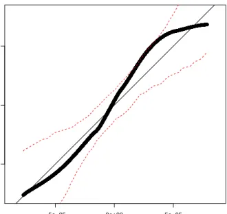
Baddeleyet al. (2005) also consider a Q-Q plotcomparing empirical quan-tiles ofs(u,x) with corresponding expected empirical quantiles estimated from
s(u,x(1)), . . . , s(u,x(n)), where x(1), . . . ,x(n) are simulations from the fitted
model. This is done using a grid of fixed locationsuj ∈W, j = 1, . . . , J. For
eachk = 0, . . . , n, where x(0) =x is the data, we sort s(k)
j =s(uj,x(k)), j =
1, . . . , Jto obtain the order statisticss([1]k)≤. . .≤s[(Jk)]. We then plots(0)[j] versus the estimated expected empirical quantilePn
k=1s (k)
[j]/n for j = 1, . . . , J. The
Q-Q plot in Figure 8 shows some deviations between the observed and estimated quantiles but each observed order statistic fall within the 95% intervals obtained from corresponding simulated order statistics.
6.1.3 Edge effects
Substantial bias and other artifacts in the diagnostic plots for residuals based on
0
200
400
600
x coordinate
−4
−2
0
1
2
cumulative sum of raw residuals
0
200
400
600
y coordinate
6
5
4
3
2
1
0
cumulative sum of raw residuals
Figure 7: Plots forCataglyphisnests based on raw residuals: mark plot (upper left), lurking variable plots for covariates given byy and xcoordinates (upper right, lower left), and smoothed residual field (lower right). Dark grey scales correspond to small values.
follows (see also Baddeleyet al., 2006b). Suppose the fitted model is Gibbs with interaction radiusR (Sections 5.3-5.4). For locationsuin W \W⊖R =∂W⊖R,
λ(u,x) may depend on points inxwhich are outside the observation windowW. Since the Papangelou conditional intensity (29) withB=W⊖Rdoes not depend
on points outside the observation window, we condition on X∂W⊖R = x∂W⊖R
and plot residuals only foru∈W⊖R. See e.g. the upper left plot in Figure 7.
For residuals based onρinstead, we have no edge effects, so no adjustment of the diagnostic tools in Section 6.1.2 is needed.
−5e−05 0e+00 5e−05
−5e−05
0e+00
5e−05
Mean quantile of simulations
data quantile
Residuals: raw
Figure 8: Q-Q plot forCataglyphisnests based on smoothed raw residual field. The dotted lines show the 2.5% and 97.5% percentiles for the simulated order statistics
6.2
Summary statistics
This section considers the more classical summary statistics such as Ripley’sK -function and the nearest-neighbour -functionG. See also Baddeley, Møller and Waagepetersen (2007) who develop residual versions of such summary statistics.
6.2.1 Second order summary statistics
Second order properties are described by the pair correlation functiong, where it is convenient if g(u, v) only depends on the distance ku−vk or at least the difference u−v (note that g(u, v) is symmetric). Kernel estimation of g
is discussed in Stoyan & Stoyan (2000). Alternatively, if g(u, v) = g(u−v) is translation invariant, one may consider the inhomogeneous reduced second moment measure(Baddeleyet al., 2000)
K(B) =
Z
B
More generally, ifg is not assumed to exist or to be translation invariant, we may define K(B) = 1 |A|E X u∈XA X v∈X\{u} 1[u−v∈B] ρ(u)ρ(v) (40)
provided thatXissecond order reweighted stationarywhich means that the right hand side of (40) does not depend on the choice ofA⊂R2, where 0<|A|<∞. Note thatK is invariant under independent thinning.
The (inhomogeneous) K-function is defined by K(r) = K(b(0, r)), r > 0. Clearly, if g(u, v) = g(ku−vk), then K is determined by K, and K(r) = 2πRr
0 sg(s) ds, so that g and K are in a one-to-one correspondence. In the
case of a stationary point process, it follows from (40) that ρK(r) has the interpretation as the expected number of further points within distancerfrom a typical point inX, andρ2K(r)/2 is the expected number of (unordered) pairs
of distinct points not more than distancerapart and with at least one point in a set of unit area (Ripley, 1976). A formal definition of ‘typical point’ is given in terms of Palm measures, see e.g. Møller & Waagepetersen (2003b). For a Poisson process,K(r) =πr2.
In our experience, non-parametric estimation ofKis more reliable than that ofg, since the latter involves kernel estimation, which is sensitive to the choice of the band-width. Various edge corrections have been suggested, the simplest and most widely applicable being
ˆ K(r) = 6 = X u,v∈x 1[ku−vk ≤r] ˆ ρ(u)ˆρ(v)|W ∩Wu−v| (41)
whereWu isW translated by u, and ˆρis an estimate of the intensity function.
The choice of ˆρis crucial since this determines how much variation is attributed to inhomogeneity rather than random clustering. In general we prefer to use a parametric estimate of the intensity function. Another possibility is the non-parametric estimate ofρgiven in (35) but the degree of clustering exhibited by the resulting estimate ˆK(r) is very sensitive to the choice of kernel band-width. An estimate of theK-function for the tropical rain forest trees obtained with a parametric estimate of the intensity function (see Example 8.1) is shown in Figure 9. The plot also shows theoreticalK-functions for fitted log Gaussian Cox, Thomas, and Poisson processes, where all three processes share the same intensity function (details are given later in Example 8.3). The trees seem to form a clustered point pattern since the estimatedK-function is markedly larger
than the theoreticalK-function for a Poisson process. 0 20 40 60 80 100 0 10000 20000 30000 40000 r K(r) Estimate Poisson Thomas LGCP
Figure 9: Estimated K-function for tropical rain forest trees and theoretical
K-functions for fitted Thomas, log Gaussian Cox, and Poisson processes. One often considers the L-function L(r) =p
K(r)/π, which at least for a stationary Poisson process is a variance stabilizing transformation whenK is estimated by non-parametric methods (Besag, 1977). Moreover, for a Poisson process, L(r) = r. In general, at least for small distances, L(r) > r indicates aggregation andL(r)< r indicates regularity. Usually when a model is fitted, ˆ
L(r) =
q
ˆ
K(r)/π or ˆL(r)−r is plotted together with the average and 2.5% and 97.5% quantiles based on simulated ˆL-functions under the fitted model; we refer to these bounds as 95% envelopes. Examples are given in the right plots of Figures 11 and 12.
Estimation of third-order properties and of directional properties (so-called directionalK-functions) is discussed in Stoyan & Stoyan (1995), Møller et al. (1998), Schladitz & Baddeley (2000), and Guan, Sherman & Calvin (2006).
6.2.2 Interpoint distances
In order to interpret the following summary statistics based on interpoint dis-tances, we assume stationarity ofX. Theempty space functionF is the distri-bution function of the distance from an arbitrary location to the nearest point inX,
F(r) = P(X∩b(0, r)6=∅), r >0.
Thenearest-neighbour function is defined by
G(r) = 1
ρ|W|E X
u∈X∩W
1[(X\ {u})∩b(u, r)], r >0,
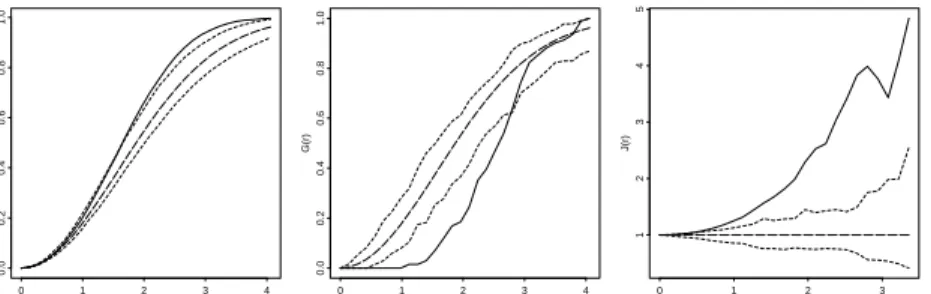
which has the interpretation as the cumulative distribution function for the distance from a ‘typical’ point inXto its nearest-neighbour point inX. Thus, for small distances,G(r) andρK(r) are closely related. For a stationary Poisson process,F(r) =G(r) = 1−exp(−πr2). In general, at least for small distances, F(r)> G(r) indicates aggregation and F(r)< G(r) indicates regularity. Van Lieshout & Baddeley (1996) study the nice properties of theJ-functiondefined byJ(r) = (1−G(r))/(1−F(r)) for F(r)<1.
Non-parametric estimation ofFandGaccounting for edge effects is straight-forward using border methods, see e.g. Møller & Waagepetersen (2003b). An estimate ofJ is obtained by plugging in the estimates ofF andGin the expres-sion forJ. We combine the estimates to obtain an estimate ofJ. Estimates of
F,G, andJ for the positions of Norwegian spruces shown in Figure 10 provide evidence of repulsion. r F(r) 0 1 2 3 4 0.0 0.2 0.4 0.6 0.8 1.0 r G(r) 0 1 2 3 4 0.0 0.2 0.4 0.6 0.8 1.0 r J(r) 0 1 2 3 1 2 3 4 5
Figure 10: Left to right: estimated F, G, andJ-functions for the Norwegian spruces (solid lines) and 95% envelopes calculated from simulations of a homo-geneous Poisson process (dashed lines) with expected number of points equal to the observed number of points. The long-dashed curves show the theoretical values ofF,G, andJ for a Poisson process.
7
Likelihood-based inference and MCMC
meth-ods
Computation of the likelihood function is usually easy for Poisson process mod-els (Section 7.1), while the likelihood contains an unknown normalizing constant for Gibbs point process models, and is given in terms of a complicated integral for Cox process models. Using MCMC methods, it is now becoming quite feasi-ble to compute accurate approximations of the likelihood function for Gibbs and Cox process models (Sections 7.2 and 7.3). However, the computations may be time consuming and standard software is yet not available. Quick non-likelihood approaches to inference are reviewed in Section 8.
7.1
Poisson process models
For a Poisson process with a parameterized intensity functionρθ, the log
likeli-hood function is l(θ) =X u∈x logρθ(u)− Z W ρθ(u) du, (42)
cf. (18), where in general numerical integration is needed to compute the in-tegral. A clever implementation for finding the maximum likelihood estimate (MLE) numerically, based on software for generalized linear models (Berman and Turner, 1992), is available in spatstat when the intensity function is of the log linear form (7).
Rathbun & Cressie (1994) study increasing domain asymptotics for inhomo-geneous Poisson point processes and provide fairly weak conditions for asymp-totic normality of the MLE in the case of a log linear intensity function. Waa-gepetersen (2007) instead suggests asymptotics for a fixed observation window when the intercept in the log linear intensity function tends to infinity, and the only condition for asymptotic normality of the MLE of the remaining parame-ters is positive definiteness of the observed information matrix. Inference for a log linear Poisson process model is exemplified in Example 8.1.
7.2
Gibbs point process models
We restrict attention to parametric models for Gibbs point processes X as in Sections 5.3–5.4, assuming that the interaction radiusR is finite and the con-ditional intensity is on the log linear form (25) (no matter whetherX is finite
or infinite). We assume to begin with thatRis known.
First, suppose that the observation windowW coincides withS. The density is then on exponential family form
fθ(x) = exp(t(x)θT)/cθ
wheretis given by (26) andcθ is the unknown normalizing constant. The score
function and observed information are
u(θ) =t(x)−Eθt(X), j(θ) = Varθt(X),
where Eθ and Varθ denote expectation and variance with respect toX∼fθ.
Consider a fixed reference parameter value θ0. The score function and
ob-served information may then be evaluated using theimportance sampling for-mula
Eθk(X) = Eθ0
k(X) exp t(X)(θ−θ0)T/(cθ/cθ0) (43)
withk(X) given byt(X) ort(X)Tt(X). The importance sampling formula also
yields
cθ/cθ0 = Eθ0
exp t(X)(θ−θ0)T. (44)
Approximations of the likelihood ratiofθ(x)/fθ0(x), score, and observed
infor-mation are then obtained by Monte Carlo approxiinfor-mation of the expectations
Eθ0[· · ·] using MCMC samples fromfθ0, see Section 9.2.
Thepath sampling identity(e.g. Gelman and Meng, 1998) log(cθ/cθ0) =
Z 1
0
Eθ(s)t(X)(dθ(s)/ds)Tds (45)
provides an alternative and often numerically more stable way of computing a ratio of normalizing constants. Hereθ(s) is a differentiable curve, e.g. a straight line segment, connectingθ0=θ(0) and θ =θ(1). The log ratio of normalizing
constants is approximated by evaluating the outer integral in (45) using e.g. the trapezoidal rule and the expectation using MCMC methods (Berthelsen & Møller, 2003; Møller & Waagepetersen, 2003b).
Second, suppose thatWis strictly contained inSand letfW,θ(x|x∂W) denote
the conditional density ofXW givenX∂W =x∂W. The likelihood function
may be computed using a missing data approach, see Geyer (1999) and Møller & Waagepetersen (2003b). A simpler but less efficient alternative is the border method, considering the conditional likelihood function
fW⊖R,θ(xW⊖R|x∂W⊖R)
where the score, observed information, and likelihood ratios may be computed by analogy with the W = S case, cf. Sections 5.3–5.4. These and other ap-proaches for handling edge effects are discussed in Møller & Waagepetersen (2003b).
For a fixedR, the approximate (conditional) likelihood function can be max-imized with respect toθusing Newton-Raphson updates. In our experience the Newton-Raphson updates converge quickly, and in the examples below, the computing times for obtaining a MLE are modest — less than half a minute. MLE’s ofR are often found using a profile likelihood approach, since the like-lihood function is typically not differentiable and log concave as a function of
R.
Asymptotic results for MLE’s of Gibbs point process models are reviewed in Møller and Waagepetersen (2003b) but these results are derived under restric-tive assumptions of stationarity and weak interaction. According to standard asymptotic results, the inverse observed information provides an approximate covariance matrix of the MLE, but if one is suspicious about the validity of this approach, an alternative is to use a parametric bootstrap.
Example 7.1. (Maximum likelihood estimation for overlap interaction model) For the overlap interaction model in Example 5.1, Møller & Waagepetersen (2003b) compute maximum likelihood estimates using both missing data and conditional likelihood approaches. LettingW = [0,56]×[0,38], the conditional likelihood approach is based on the trees with locations inW⊖2b, since trees with
locations outsideW do not interact with trees located insideW⊖2b. The
condi-tional MLE is given by ( ˆβ1, . . . ,βˆ6) = (−1.02,−0.41,0.60,−0.67,−0.58,−0.22)
and ˆψ = −1.13. Confidence intervals for ψ obtained from the observed in-formation and a parametric bootstrap are [−1.61,−0.65] and [−1.74,−0.79], respectively. As expected, due to the repulsive interaction term in the condi-tional intensity (30), the ˆβk tend to be larger than expected under the Poisson
model withψ= 0. This is illustrated in Figure 11 (left plot), where the exp( ˆβk)
are shown together with relative frequencies of trees within each of the six size classes (the frequencies are proportional to the MLE of the exp(βk) under the
Poisson model). The fitted overlap interaction process seems to capture well the second order characteristics for the point pattern of tree locations, see Figure 11 (right plot). 1 2 3 4 5 6 r L(r)-r 0 5 10 15 -1.5 -1.0 -0.5 0.0
Figure 11: Model assessment for Norwegian spruces (Example 7.1). Dark grey bars: frequencies of trees for the six size classes (scaled so that light and dark bars are of the same height for the first class). Light gray bars: MLE of exp(βk),
k = 1, . . . ,6. Right plot: estimated L(r)−r function for spruces (solid line) and average and 95% envelopes computed from simulations of fitted overlap interaction model (dashed lines).
Example 7.2. (Maximum likelihood estimation for ants nests) H¨ogmander & S¨arkk¨a (1999) consider a subset of the data in Figure 5 within a rectangular region, and they condition on the observed number of points for the two species when computing MLE’s and MPLE’s for the hierarchical model described in Example 5.2, whereby the parametersβM and βC vanish. Instead we fit the
hierarchical model to the full data set, we do not condition on the observed number of points, and we set rCM = 0. No edge correction is used for our
MLE’s, but in Example 8.2 we compare maximum pseudo-likelihood estimates (Section 8.1) obtained both with and without edge correction. The MLE’s
ˆ
βM = −8.39 and ˆψM = −0.06 indicate a weak repulsion within the Messor
nests, and the MLE’s ˆβC = −9.24, ˆψCM = 0.04, and ˆψC = −0.39 indicate
positive association betweenMessorandCataglyphisnests, and repulsion within theCataglyphisnests. Confidence intervals forψCM are [−0.20,0.28] (based on
observed information) and [−0.16,0.30] (parametric bootstrap). To avoid the phase transition property of the Strauss hard core process (Example 5.2), we restrictψC ≤0 in the Monte Carlo computations for the bootstrap simulated
data sets. The results in H¨ogmander & S¨arkk¨a (1999) differ from ours, since they estimate a stronger repulsion within theCataglyphisnests and a weak repulsion between the two species. This seems partly due to the fact that H¨ogmander & S¨arkk¨a (1999) use a smaller observation window which excludes a pair of very closeCataglyphisnests, see also Example 8.2.
7.3
Cox process models
We consider MLE for shot noise Cox processes and log Gaussian Cox processes. In the case of a shot noise Cox process (Section 4.2.2), suppose that the parameter vector θ = (α, ω) consists of components α and ω parameterizing respectively the intensity function ζα of Φ and the kernel k(c,·) = k(c,·;ω).
Let f(x|Λ) denote the Poisson density of XW given Λ(·) = Λ(·;Φ, ω). For
simplicity assume that k is of bounded support, i.e. there exists a bounded region ˜W = ˜Wω ⊃W so thatk(c, u;ω) = 0 wheneverc∈R2\W˜ and u∈W.
The likelihood
L(θ) = Eαf x|Λ(·;Φ, ω)= Eαf x|Λ(·;ΦW˜, ω)
is then given in terms of an expectation with respect to the Poisson process
ΦW˜ = {(c, γ) ∈ Φ|c ∈ W˜}. We assume moreover that R0∞ζα(c, γ)dγ < ∞
wheneverc∈W˜. TherebyΦW˜ is finite and we letfW˜(·;α) denote the Poisson
process density of ΦW˜. Choose a reference parameter value θ0 = (α0, ω0).
ThenL(θ) is the normalizing constant of f(x|Λ(·;ϕ, ω))fW˜(ϕ;α) viewed as an
unnormalized density for the conditional distribution of ΦW˜ given XW = x.
Consequently, in analogy with (44),
L(θ)/L(θ0) = Eα0 " f x|Λ(·; ΦW˜, ω) fW˜(ΦW˜;α) f x|Λ(·; ΦW˜, ω0)fW˜(ΦW˜;α0) XW =x # (46)
which can be approximated using samples from the conditional distribution of
ΦW˜ givenXW =xandθ=θ0. Let
Vθ,x(ΦW˜) = d log f(x|Λ(·;ΦW˜, ω))fW˜(ΦW˜;α)/dθ.
The score function and observed information are given by
and j(θ) =−Eθ dVθ,x(ΦW˜)/dθT|XW =x −Varθ[Vθ,x(ΦW˜)|XW =x].
Approximations of these conditional expectations can be obtained by applying importance sampling (Section 8.6.2 in Møller & Waagepetersen, 2003b). Sam-ples from the conditional distribution of ΦW˜ can be generated using MCMC,
see Section 9.2.
For a log Gaussian Cox process (Section 4.2.1), we consider a finite partition
Ci, i ∈ I, of W and approximate the Gaussian process (Ψ(u))u∈W by a step
function with value Ψ(ui) within Ci, where ui is a representative point inCi.
We then proceed in a similar manner as for shot noise Cox processes, but now computing conditional expectations with respect to the finite Gaussian vector (Ψ(ui))i∈I givenXW =x. Conditional samples of (Ψ(ui))i∈I may be obtained
using Langevin-Hastings MCMC algorithm