Multi-dimensional local binary pattern texture descriptors and their application for medical image analysis

(1)

Multi-Dimensional Local Binary Pattern Texture

Descriptors and their Application for Medical

Image Analysis

by

Niraj P. Doshi

A Doctoral Thesis

Submitted in partial fulfilment

of the requirements for the award of

Doctor of Philosophy

of

Loughborough University

(2)

Acknowledgement

While pursuing ones lifetime goals, many helpful and sympathetic hands come forward to help, knowingly as well as unknowingly. Often only when the goals are achieved, one becomes aware of that help.

I take this opportunity to express my deep sense of gratitude towards my super-visors Dr. Gerald Schaefer for his sincere support, patience, and encouragement throughout my research and for valuable guidance provided in writing and com-pleting this thesis. It is not often that one finds a supervisors and colleagues that always find the time for listening to the little problems and roadblocks that un-avoidably crop up in the course of performing research. His technical and editorial advice was essential to the completion of this thesis and has taught me innumer-able lessons and insights into the workings of academic research in general. I also like to thank Dr. Eran Edirisinghe for his help and support during my studies.

I am also very much thankful technical and clerical staff members of Depart-ment of Computer Science for their guidance towards the successful completion of this thesis. I would also specially like to thank all members of the Digital Ima-ging Research Lab, Loughborough University, and my friends Vaibhav, Amey and Giounona for their support and valuable guidance while completing my research project.

I have a deep regard for my wife, Sneha who has always been supportive of me and provided me with immeasurable love and inspiration. Above all I must thank my wife for all the sacrifices made on my behalf during my studies. I am profoundly thankful to my parents for creating all the opportunities for me and for their love, affection, and encouragement. I should express my sincere gratitude for my sister Pooja, parents-in-law and the rest of the family for their extensive love, support and friendship.

Finally, and perhaps most importantly, I am forever indebted to my sister Jagruti , her husband Rupesh, kids Krish and Arya who energised, encouraged and support me during my research. I wish to thank them for their support, understanding, endless patience and encouragement when it was most required.

(3)

Abstract

Multi-Dimensional Local Binary Patterns

Texture Descriptors and their Application for

Medical Image Analysis

Niraj P. Doshi, Oct 2014.

Texture can be broadly stated as spatial variation of image intensities. Tex-ture analysis and classification is a well researched area for its importance to many computer vision applications. Consequently, much research has focussed on deriv-ing powerful and efficient texture descriptors. Local binary patterns (LBP) and its variants are simple yet powerful texture descriptors. LBP features describe the texture neighbourhood of a pixel using simple comparison operators, and are often calculated based on varying neighbourhood radii to provide multi-resolution texture descriptions.

A comprehensive evaluation of different LBP variants on a common benchmark dataset is missing in the literature. This thesis presents the performance for dif-ferent LBP variants on texture classification and retrieval tasks. The results show that multi-scale local binary pattern variance (LBPV) gives the best performance over eight benchmarked datasets. Furthermore, improvements to the Dominant LBP (D-LBP) by ranking dominant patterns over complete training set and Com-pound LBP (CM-LBP) by considering 16 bits binary codes are suggested which are shown to outperform their original counterparts.

The main contribution of the thesis is the introduction of multi-dimensional LBP features, which preserve the relationships between different scales by build-ing a multi-dimensional histogram. The results on benchmarked classification and retrieval datasets clearly show that the multi-dimensional LBP (MD-LBP) im-proves the results compared to conventional multi-scale LBP. The same principle is applied to LBPV (MD-LBPV), again leading to improved performance. The proposed variants result in relatively large feature lengths which is addressed using three different feature length reduction techniques. Principle component analysis (PCA) is shown to give the best performance when the feature length is reduced to match that of conventional multi-scale LBP.

(4)

CHAPTER 0. ABSTRACT 4

The proposed multi-dimensional LBP variants are applied for medical image analysis application. The first application is nailfold capillary (NC) image classi-fication. Performance of MD-LBPV on NC images is highest, whereas for second application, HEp-2 cell classification, performance of MD-LBP is highest. It is ob-served that the proposed texture descriptors gives improved texture classification accuracy.

(5)

List of Figures

1.1 Image classification example . . . 1

1.2 Texture spectrum . . . 3

2.1 Texture example . . . 8

2.2 Texture and Scale relationship . . . 10

2.3 Co-occurrence matrix . . . 13

2.4 Texture synthesis using texels . . . 15

2.5 Example of Gabor filter bank . . . 21

2.6 Texture classification example. . . 23

2.7 Example of texture analysis for image segmentation . . . 25

3.1 Circular LBP . . . 28

3.2 Rotation invariant LBP . . . 29

3.3 Uniform LBP . . . 29

3.4 Rotation invariant uniform patterns . . . 30

3.5 Multi-scale LBP . . . 31 3.6 Hierarchical multiscale LBP . . . 34 3.7 Completed LBP . . . 35 3.8 Three patch LBP . . . 37 3.9 Four patch LBP . . . 38 3.10 Multi-block LBP . . . 39 3.11 Transition LBP . . . 39

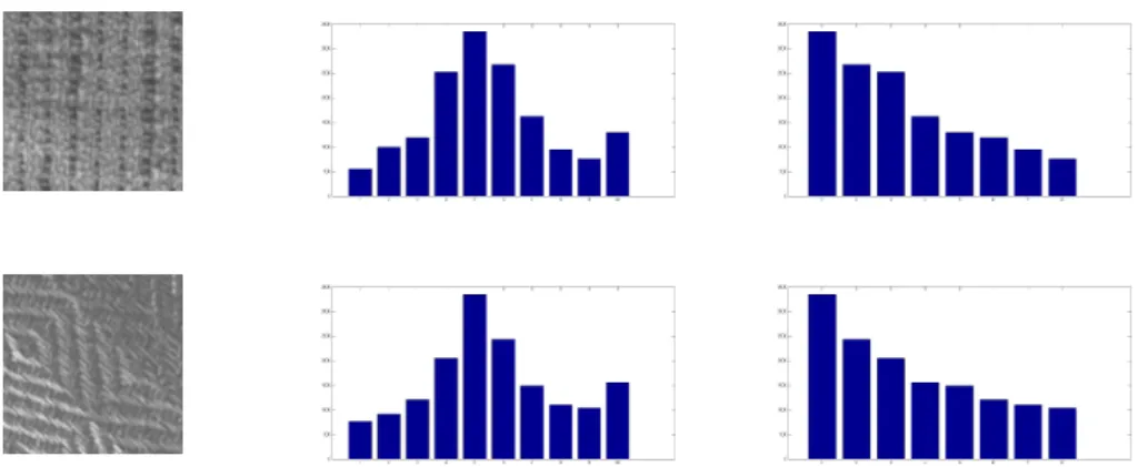
4.1 Sample LBP and D-LBP histograms . . . 46

4.2 Classification . . . 47

4.3 Support Vector Machines . . . 48

4.4 Support Vector Machine Kernel . . . 48

4.5 Sample texture images of Outex TC 00 dataset . . . 50

4.8 Comparison of LBP and LBPri _{. . . .} ₅₃

(10)

LIST OF FIGURES 10

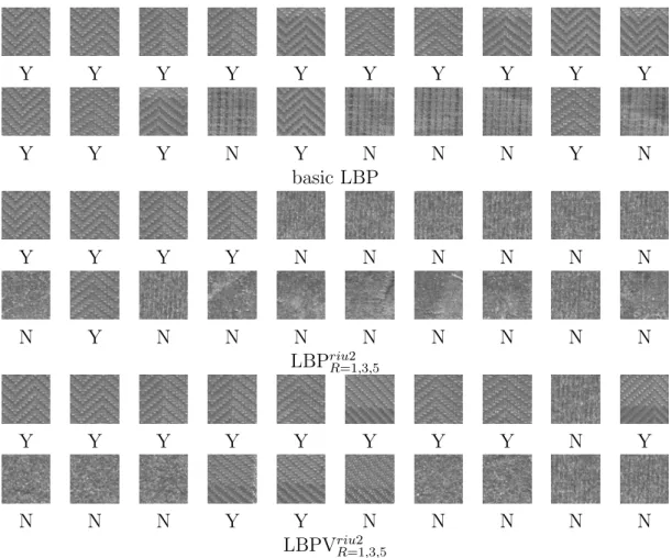
4.9 Sample texture classification of the TC 10 dataset . . . 56

4.10 Sample texture retrieval results . . . 59

5.1 Example of multi-scale LBP . . . 63

5.2 Multi-dimension LBP (MD-LBP) . . . 64

5.3 Multi-dimension LBPV (MD-LBPV) . . . 65

5.4 Example of LBP and MD-LBP histograms. . . 67

6.1 PCA for dimension reduction . . . 73

6.2 Accuracy vs. feature length graph for D-MD-LBPriu_R₌₁2_,₃ . . . 75

6.3 Accuracy vs. feature length graph for D-PCA-MD-LBPriu_R₌₁2_,₃ . . . . 76

6.4 Accuracy vs. feature length graph for PCA-MD-LBPriu2 R=1,3 . . . 78

7.1 Sample SD patterns . . . 81

7.2 Bilateral enhancer filtering . . . 87

8.1 Sample HEp-2 cell images . . . 94

8.2 Sample HEp-2 cell image and its three channels . . . 96

(11)

List of Tables

3.1 Summary on different LBP variants. . . 43

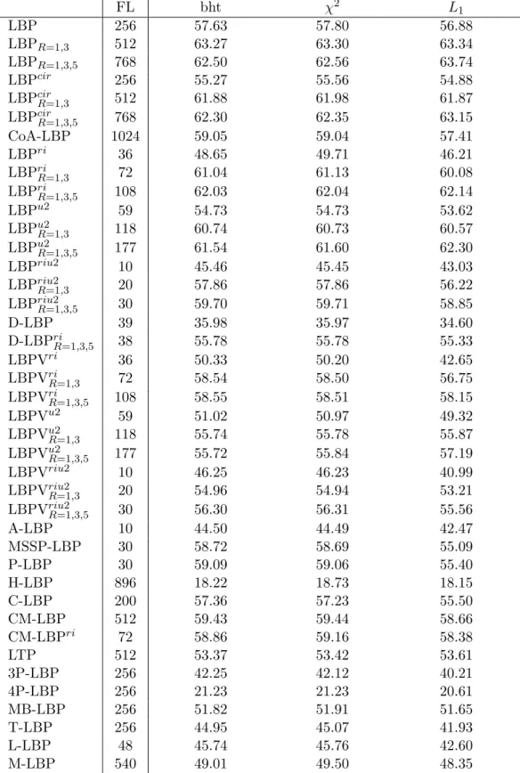
4.1 Texture classification results on all LBP variants . . . 54

4.2 Texture retrieval results on all LBP variants . . . 58

4.3 Texture classification results on improved Compund LBP . . . 59

4.4 Texture retrieval results on improved Compound LBP . . . 60

4.5 Texture classification results on improved Dominant LBP . . . 60

4.6 Texture retrieval results on Improved Dominant LBP . . . 60

5.1 MD-LBP texture classification results. . . 66

5.2 MD-LBP texture retrieval results. . . 66

5.3 MD-LBPV texture classification results. . . 68

5.4 MD-LBPV texture retrieval results. . . 69

6.1 Feature length reduction using dominant features at radiiR ={1,3}. 75 6.2 Feature length reduction using dominant features at radii R = {1,3,5}. . . 75

6.3 Feature length reduction using PCA on dominant features at radii R={1,3}. . . 76

6.4 Feature length reduction using PCA on dominant features at radii R={1,3,5}. . . 77

6.5 Feature length reduction using PCA at radiiR ={1,3}. . . 78

6.6 Feature length reduction using PCA at radiiR ={1,3,5}. . . 78

7.1 Experimental results, expressed in terms of Pratt’s figure of merit. . 85

7.2 Nailfold capillary analysis using LBPriu2 R=1,3 . . . 88

7.3 Nailfold capillary analysis using LBPriu_R₌₁2_,₃_,₅ . . . 88

7.4 Nailfold capillary analysis using MD-LBPriu_R₌₁2_,₃ . . . 89

7.5 Nailfold capillary analysis using MD-LBPriu_R₌₁2_,₃_,₅ . . . 89

7.6 Nailfold capillary analysis using LBPVriu_R₌₁2_,₃ . . . 89

7.7 Nailfold capillary analysis using LBPVriu2 R=1,3,5 . . . 90

7.8 Nailfold capillary analysis using MD-LBPV(M AX)riu2 R=1,3 . . . 90

(12)

LIST OF TABLES 12

7.9 Nailfold capillary analysis using MD-LBPV(M AX)riu2

R=1,3,5 . . . 91

7.10 Accuracy in percentage for finger classification and patient classi-fication. . . 91

8.1 Classification accuracy of HEp-2 cell images from the ICPR 2012 contest dataset using two radii LBP. . . 97

8.2 Classification accuracy of HEp-2 cell images from the ICPR 2012 contest dataset using three radii LBP. . . 97

8.3 Classification accuracy of HEp-2 cell images from the ICPR 2012 contest dataset using PCA-MD-LBP and PCA-MD-LBPV. . . 98

8.4 Top classification results on ICPR test data at cell level. . . 99

8.5 Confusion matrix for MD-LBPriu2 R=1,3,5 method. . . 99

B.1 Confusion matrix for LBPriu2 R=1,3 on TC 00 dataset. . . 123

B.2 Confusion matrix for MD-LBPriu2 R=1,3 on TC 00 dataset. . . 123

B.3 Confusion matrix for LBPriu2 R=1,3 on TC 10 dataset. . . 124

B.4 Confusion matrix for MD-LBPriu_R₌₁2_,₃ on TC 10 dataset. . . 124

B.5 Confusion matrix for LBPriu_R₌₁2_,₃ on TC 12 dataset. . . 125

B.6 Confusion matrix for MD-LBPriu_R₌₁2_,₃ on TC 12 dataset. . . 125

B.7 Confusion matrix for LBPriu_R₌₁2_,₃_,₅ on TC 00 dataset. . . 126

B.8 Confusion matrix for MD-LBPriu2 R=1,3,5 on TC 00 dataset. . . 126

B.9 Confusion matrix for LBPriu2 R=1,3,5 on TC 10 dataset. . . 127

B.11 Confusion matrix for LBPriu2 R=1,3,5 on TC 12 dataset. . . 128

B.13 Confusion matrix for LBPVriu2 R=1,3 on TC 00 dataset. . . 129

B.14 Confusion matrix for MD-LBPVriu_R₌₁2_,₃ on TC 00 dataset. . . 129

B.15 Confusion matrix for LBPVriu_R₌₁2_,₃ on TC 10 dataset. . . 130

B.16 Confusion matrix for MD-LBPVriu_R₌₁2_,₃ on TC 10 dataset. . . 130

B.17 Confusion matrix for LBPVriu2 R=1,3 on TC 12 dataset. . . 131

B.18 Confusion matrix for MD-LBPVriu2 R=1,3 on TC 12 dataset. . . 131

B.19 Confusion matrix for LBPVriu2 R=1,3,5 on TC 00 dataset. . . 132

B.20 Confusion matrix for MD-LBPVriu2 R=1,3,5 on TC 00 dataset. . . 132

B.21 Confusion matrix for LBPVriu2 R=1,3,5 on TC 10 dataset. . . 133

B.22 Confusion matrix for MD-LBPVriu2 R=1,3,5 on TC 10 dataset. . . 133

B.23 Confusion matrix for LBPVriu_R₌₁2_,₃_,₅ on TC 12 dataset. . . 134

(13)

Abbreviations

LBP Local Binary Pattern

NC Nailfold Capillary

HEp-2 Human Epithelial Cell Type 2

D-LBP Dominant LBP

LBPV LBP Variance

A-LBP Adaptive LBP

MSSP-LBP Multi-scale Spatial Pyramid LBP

P-LBP Pyramid LBP

H-LBP Hierarchical Multi-scale LBP

C-LBP Completed LBP

CM-LBP Compound LBP

LTP Local Ternary Patterns

3P-LBP Three Patch LBP 4P-LBP Four Patch LBP MB-LBP Multi-block LBP T-LBP Transition LBP L-LBP Line LBP M-LBP Monogenic LBP

SVM Support Vector Machine

MD-LBP Multi-dimensional LBP

MD-LBPV Multi-dimensional LBP Variance

PCA Principal Component Analysis

SD Scleroderma

Notations

LBPri _{LBP with rotation invariant mappings}

LBPu2 LBP with uniform mappings

LBPriu2 _{LBP with rotation invariant uniform mappings}

LBPR LBP with radius R

(14)

Chapter 1

Introduction

Object detection and classification is most important in several image processing and computer vision applications. Is there a human face in this image and if so, who is it? Is there any particular object present in the image and if it is, then where exactly? How many such objects are there?

Not only this, in medical image analysis there are several questions which are related to human health and are equally important. Is any abnormality present

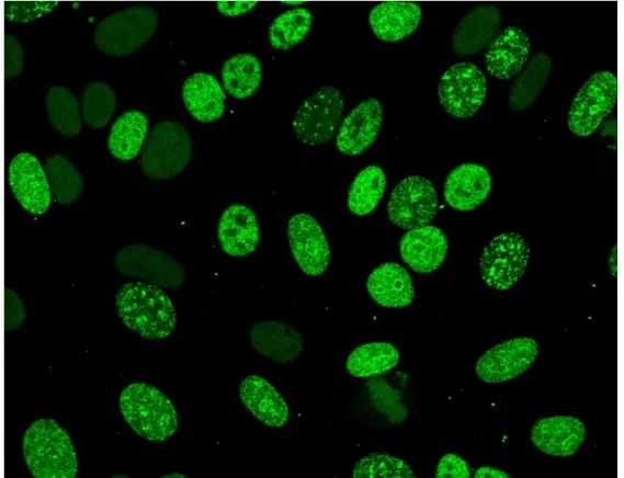
in the image? For example, in Figure 1.1 a typical problem of human cell

clas-sification is presented. Each cell in the image has to be analysed by an expert which is a time consuming and monotonous task. The expert has to answer

ques-Figure 1.1: Example of medical image classification

(15)

CHAPTER 1. INTRODUCTION 2

tions like, how many defective cells are there in the image? What type of cells are present? Sooner or later, demand to automate the detection and classification in these types of questions, will be there. Consequently, good quality descriptors and strong classifiers are needed. The researchers are working on texture based descriptors and are developing powerful descriptors to meet real life challenges.

Since the pioneering work in [55], good results have been reported in difficult

visual classification tasks such as medical image processing, industrial surface in-spection, contented based image retrieval and face recognition. This work reports the importance of clusters formed by proximate points of uniform brightness in visual discrimination. Although, human visual system is a source of inspiration, it is a difficult challenge for the researchers. The human visual system can eas-ily react to the change in ambient conditions and hence can analyse the object accurately even in poor illumination conditions.

In practical life, changes in orientation, scale, illumination and other confound-ing imagconfound-ing factors are still a big challenge for automatic texture analysis. The texture images captured with two different lighting conditions, or different camera positions at times can appear completely different. The researchers have put ex-tensive effort to solve these problems and have developed powerful machine learn-ing and texture classification algorithms. Despite significant efforts, the maxim garbage in, garbage out still applies: if descriptive features are not provided, the good classification will not be achieved. This thesis worked on the texture descriptors and investigate some of the descriptors, especially local binary pattern based descriptors and proposed multi-dimensional texture descriptors for better texture analysis.

This chapter presents a brief introduction on texture analysis and its role in computer vision algorithms. Subsequently the research motivation is presented in

section1.2, followed by the aim and objectives of the research. The contributions

of the thesis are listed in section 1.4 and finally the organisation of the thesis is

given in the last section of this chapter.

1.1

Texture

Texture can be broadly defined as the visual or tactile surface characteristics and appearance of the object. Unfortunately, no one has so far been able to define digital texture in mathematical terms. In general, textures are formed by a single surface via variations in shape, illumination, shadows, absorption and reflectance.

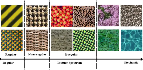
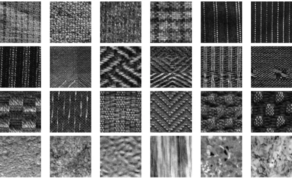
In Figure 1.2, we present examples of variety of texture patterns that can

be used to describe a wide variety of surfaces such as terrain, plants, minerals, walls, fur, skin and some natural phenomena like weathering and corrosion. These

(16)

CHAPTER 1. INTRODUCTION 3

Figure 1.2: Texture spectrum

texture samples can be categorised into four texture patterns regular, near-regular, irregular and stochastic. These form a texture spectrum in which the perceptual structural regularity varies continuously from being regular to random.

Analysis of these textures has been a topic of intensive research since the 1960s, and a wide variety of techniques for discriminating textures have been

proposed in the literature. Chapter 2 and Chapter 3 discuss in detail different

texture descriptors and give a grouping for these descriptors. These descriptors are successfully utilised in many applications including texture classification, texture retrieval, texture synthesis and segmentation.

1.2

Motivation of Research

Texture analysis and classification algorithms are employed in many computer vis-ion applicatvis-ions including biomedical image analysis, industrial surface inspectvis-ion, content-based image retrieval, face analysis, etc. Consequently, much research has focussed on deriving powerful and efficient texture descriptors. Even though colour is an important cue in interpreting images, textures can be good axillary features to interpret images.

Thus textures are useful for understanding natural image scenes, medical image analysis, industrial surface inspection, etc. To meet the requirements of real-world applications, texture operators should be computationally cheap and robust against variations in the appearance of a texture. These variations may be caused by varying illumination, different viewing positions, shadows, etc. While achieving the invariance to ambient conditions, texture should retain their discrimination power.

(17)

motiva-CHAPTER 1. INTRODUCTION 4

tion for the further research in LBP based texture descriptors. LBP based texture algorithms have gained significant popularity in recent years. LBP, first

intro-duced in [78] and generalised in [79], represents a relatively simple yet powerful

texture descriptor, describing the relationship of a pixel to its immediate neigh-bourhood. Successively, many variants of LBP were introduced aiming to outper-form the earlier LBP variant or to address various limitations. These variants are sometimes designed to perform on specific application. For example Multi-block

LBP [126] has been introduce for face detection, Dominant LBP [64] is for baby

facial expressions classification.

In the literature variety of LBP variants are proposed, however, their per-formance on a common benchmark dataset is missing. With this motivation, 19 different LBP variants are discussed and their performance on eight texture clas-sification datasets and one texture retrieval dataset is benchmarked in this thesis.

The performance of multi-scale LBP as reported in [79, 67, 94] has provided

fur-ther motivation to experiment and investigate some real life challenges in medical image understanding. Building multi-dimensional histograms for colour images is one of the proven ways to describe colour images. This approach is applied to multi-scale LBP in this thesis and their performance is benchmarked. Applying texture descriptors to practical scenarios is also a motivation of the work presented in this thesis, and thus multi-dimensional LBP features are proposed for medical image classification. The work reported in this thesis is limited to two dimensional texture images.

1.3

Aim and Objectives

The aim of this research is “to propose novel LBP variants which improve the texture description of an image and use them for medical image analysis”. The specific research objectives are listed below:

• To study existing Local Binary Pattern variants and suggest novel ideas for

their improvement.

• To evaluate and benchmark different LBP variants on a common texture

dataset.

• To evaluate the improvements suggested to LBP variants and address the

shortcoming of the descriptor.

• To apply multi-dimension histograms to LBP.

• To automate the classification of nailfold capillary images using multi-dimensional

(18)

CHAPTER 1. INTRODUCTION 5

• To automate the classification of HEp-2 cell images using multi-dimensional

LBP features.

1.4

Contributions

The following original contributions have been made by the research presented in this thesis. A list of publications are included in Appendix A, and are referenced as A.1 to A.25.

A. Benchmark different LBP variants and propose improvements to LBP variants [A.01-A.05]

In Chapter 3, the original LBP descriptor, its circular version, rotation invariant

and uniform mappings for circular LBP along with 14 different variants are

stud-ied. Chapter 4 benchmarks all these variants on eight texture datasets designed

for classification and one texture dataset designed for retrieval. Furthermore, an

improvement to the compound LBP (CM-LBP) [4] is suggested by considering a

16-bit description code and an improvement to Dominant LBP (D-LBP) [64] by

improving the process of finding dominant patterns. In total, the performance of 46 LBP variants are reported. It is found that, the suggestion for improving CM-LBP and D-LBP improved the classification performance. It is observed that

multi-scale LBP variance (LBPV) [41] gives highest overall accuracy over eight

classification datasets, while multi-scale LBP works better on the retrieval data-set.

B. Proposed Multi-Dimensional LBP (MD-LBP) and Multi-Dimensional LBP variance (MD-LBPV) texture descriptor [A.06-A.07]

From the results in Chapter 4, it is observed that multi-scale LBP significantly

improves the classification and retrieval accuracy. However, it is found that build-ing a multi-dimensional histogram will result in better performance as it preserves the spatial relationships between the scales. This approach is further extended

for the LBP variance descriptor [41] and six methods to build a multi-dimension

LBPV histogram are proposed. The multi-dimension approach is a significant contribution of this thesis.

C. Feature length reduction for multi-dimensional LBP features [A.08-A.12]

The multi-dimensional LBP features perform very well compared to multi-scale LBP, however they generate large feature size. The high dimensional feature length generated using multi-dimensional features (MD-LBP) is reduced to an acceptable

(19)

CHAPTER 1. INTRODUCTION 6

level using three different feature length reduction methods. Here, D-LBP

sug-gested in [64] is utilised for the purpose of the feature length reduction with few

changes to the original algorithm. The principal component analysis (PCA) based feature selection approach give the highest accuracy.

D. Medical Image Analysis [A.13-A.25]

The performance of MD-LBP and MD-LBPV is evaluated on two applications. First nailfold capillary (NC) imaging techniques and computer algorithms for its automation are studied. Then a novel approach is proposed for the classification of NC images based on texture analysis. No one before has presented any texture descriptor based algorithm for classification of the NC images. From experiments it is found that MD-LBPV gives the highest performance.

Indirect immunofluorescence imaging is used for screening of HEp-2 cells. In another set of experiments, the proposed multi-dimensional LBP features are used for automatic classification of HEp-2 cells. From the results, it is found that MD-LBP features are useful for the classification of HEp-2 cells.

1.5

Organisation of Thesis

For clarity of presentation the thesis has been organised into nine chapters as de-scribed below.

Chapter 2 presents details of the existing literature on texture analysis methods and descriptors. The chapter discus different texture descriptors and categorise them into four groups. Furthermore, the application of texture analysis methods are given.

Chapter 3 concentrates on providing the background reading in the context of LBP texture descriptor and its variants that are proposed in the literature. As local binary pattern descriptor is the basis of this thesis, a detailed literature re-view on LBP is given. First, the basic LBP concept is explained together with its circular representation, rotation invariant and uniform mappings and 14 different variants are discussed in detail.

Chapters 4 presents first contribution of this thesis. The LBP descriptor and its variants discussed in Chapter 3 are benchmarked on a common texture database. In total eight classification databases and one retrieval datasets are use for bench-marking purposes. In total 46 combinations of LBP descriptors are benchmarked.

(20)

CHAPTER 1. INTRODUCTION 7

In this chapter the limitation of scale LBP is given and proposed a multi-dimensional LBP to preserve the relationships between the scales. This approach

is further extended for the LBP variance descriptor [41] and six methods to build

a multi-dimension LBPV histogram are proposed.

Chapter 6 proposes three methods to reduce the feature length of multi-dimensional LBP. The experiment shows that the PCA based approach for reducing feature length of MD-LBP descriptors gives the best performance.

Chapters 7 provides the application side of the new descriptors proposed in earlier chapters. This chapter propose a novel approach for NC image classification using a texture analysis method and shows that MD-LBPV descriptors work better for NC image classification.

Chapter 8 gives another application of medical image classification using texture descriptors. This chapter proposed to apply MD-LBP texture descriptor for clas-sification of HEp-2 cells. It is also shown that compact MD-LBP also perform very well on this dataset.

(21)

Chapter 2

Literature Review

There is, generally no accepted formal definition for textures, however image tex-ture gives us information about the spatial arrangement of colour or intensities in an image or selected region of an image. Texture is a fundamental property of natural images, and thus it is one of the important topics to study in the fields of computer vision and computer graphics. Texture analysis is a successful method used in many computer vision algorithms including medical image analysis, im-age retrieval, imim-age segmentation which requires robust and fast processing

al-gorithms. As can be seen in figure 2.1, we can recognise the texture, as it shows

characteristics variation in intensities. However, defining it is a challenge.

Texture descriptors, (possibly mathematical) representations of texture, are applied to encapsulate textural properties and study the textures. Developing powerful texture descriptors is an active research area, which addressed the chal-lenges in practical applications such as variation in rotation, illumination and scaling. This chapter presents different applications using texture analysis method and discuss in detail various kinds of texture descriptors.

2.1

Background

2.1.1

What is Texture?

The word texture comes from the Latin word textura, which means textile fabric.

The concept of texture is intuitively obvious to us, but it is hard to define. Al-though there is no formal definition, we describe texture as fine, coarse, grained, smooth, regular/irregular, directional, etc. Nevertheless, these descriptions are imprecise and non-quantitative.

Although researchers have been studying the subject since long, no one has given a widely accepted mathematical definition of texture yet. In the literature, many of the studies given try for defining texture. Some definitions of texture

(22)

CHAPTER 2. LITERATURE REVIEW 9

obtained from the literature are given below.

• “The term texture generally refers to repetition of basic texture elements called texels. The texel contains several pixels, whose placement could be periodic, quasi-periodic or random. Natural textures are generally random, whereas artificial textures are often deterministic or periodic. Texture may be coarse, fine, smooth, granulated, rippled, regular, irregular or linear” [52].

• “Texture is characterized not only by the gray value at a given pixel,but also by the gray value ‘pattern’ in a neighbourhood surrounding the pixel” [53].

• “We consider a texture to be stochastic, possibly periodic two dimensional image field” [22].

• “A region in an image has a constant texture if a set of local statistics or other local properties of the picture function are constant, slowly varying or approximately periodic” [100].

• “We may regard texture as what constitutes a macroscopic region. Its struc-ture is simply attributed to the repetitive patterns in which elements or prim-itives are arranged according to a placement rule” [108].

• “Texture has been extremely refractory to precise definition” [46].

Although there is no universally agreed definition, almost all researchers agree on the following.

• “While colour is a point property, texture is a local-neighbourhood prop-erty” [8].

• “A texture is a region that can be perceived as being spatially homogeneous in some sense” [12].

Scale is a crucial concept that must be considered when dealing with textures,

because the same texture at various scales may be perceived as different [62]. Thus,

there may be several levels of completely different textures in the same image, but

at different scales. For instance, in Figure2.2, the leaf in the left image has different

texture information and the tree made up of a number of leaves give different

information. [61] identified the following properties as playing an important role in

describing texture: uniformity, density, coarseness, roughness, regularity, linearity, directionality, direction, frequency, and phase. In the following sections it will be discovered that the perception of texture has so many different dimensions is an

(23)

CHAPTER 2. LITERATURE REVIEW 10

important reason why there is no single method of texture representation which is adequate for a variety of textures.

2.1.2

Texture Analysis Methods

Texture analysis methods were initially divided into two categories. The first one, called the statistical approach, treats textures as statistical phenomena. The formation of a texture is described by the statistical properties of the intensities and positions of pixels. The second category is known as structural approach and is based on the concept of texture primitives, often called texels or textons. Texture description is based on the vocabulary of texels and their relationship. In other words, this approach describes the complex structure using simpler primitives.

Another way of classifying texture methods has been proposed in [18].

Accord-ing to the author, modern methods either try to understand the process of texture formation, or base themselves on the theory of human perception. The earlier

di-vision of texture analysis methods is refined in [112] in which four categories were

proposed: statistical, geometrical, model based, and signal processing. Model based texture analysis methods are based on the construction of an image model that can be used not only to describe texture, but also to synthesise it. The model parameters capture the essential perceived qualities of texture. The last category is signal processing based methods, which involves the filtering of images and then frequency analysis for texture description. In the following section, texture descriptors from the above groups are discussed in details.

2.2

Texture Descriptors

A representation of texture, usually numeric, also known as texture features, is

calculated by one of the methods categorised in 2.1 and use for computer vision

applications. Certain features work better on particular applications and no single feature is suitable for all applications. It is difficult to select appropriate feature descriptors and often an empirical evaluation is required to find the most effect-ive features. One of the major problems when developing texture measures is to address invariant properties in the descriptors. It is very common in real-world environment that, for example, the illumination changes over time and causes variations in the texture appearance or rotation and scale changes are also com-mon. In the following, different texture descriptors are discussed following the

(24)

CHAPTER 2. LITERATURE REVIEW 11

2.2.1

Statistical Texture Descriptors

Statistical texture descriptors are the important qualities of texture based on the spatial distribution of the intensity values. Thus, it is one of the earliest methods suggested in the literature of texture descriptors. The easiest statistical property of texture would be to calculate the variance of the pixel value from the grey level histogram of the image.

[44] have filtered the original image with several Gaussian filters, and

construc-ted a multi-resolution intensity histogram of the image as texture features. The multi-resolution decomposition of an image is computed with Gaussian filtering and then the set of intensity histograms of the image at each image resolutions are considered for feature generation.

Another example for detecting texture properties statistically is the use of gray-level run length features to detect texture properties. A gray level run is a set of consecutive, collinear picture points having the same gray level value. The

length of the run is the number of picture points in the run [34]. A fraction of

image in runs, short run, long runs, uniformity, percentage are some parameters that can be derived from the run-length matrix as texture descriptors. E.g. for a sample image

(25)

CHAPTER 2. LITERATURE REVIEW 12

0 1 2 3

0 2 3 3

2 1 1 1

3 0 3 0

the run length matrices at 0◦ and 45◦ are generated as

0◦ 1 2 3 4 0 4 0 0 0 1 1 0 1 0 2 3 0 0 0 3 3 1 0 0 and 45◦ 1 2 3 4 0 4 0 0 0 1 4 0 0 0 2 3 0 1 0 3 3 1 0 0 respectively

Rather than using these run length matrices as it is, its characteristics features such as short run emphasis, long run emphasis, gray level non-uniformity, run length non-uniformity and run percentage can be extracted and use as texture features.

Different run-length matrices can be built for one image with various

direc-tions [104]. Texture features from run length matrices are easy to extract, but

in [20] their performance has been reported to be quite poor.

Another simple texture statistic is to calculate the autocorrelation function of the image. This can be used to assess the amount of regularity, as well as the coarseness of the texture present in the image. This function describes the texture spatial organisation by the correlation coefficient that evaluates linear

spatial relationships between primitives [112]. IfIis an image then the correlation

coefficient is given as ρ(x, y) = PN u=0 PN v=0I(u, v)I(u+x, v+y) PN u=0 PN v=0I2(u, v) (2.1)

where (x,y) is the positional differences in the (u,v) direction. This function is

related to the size of the texture primitive (i.e., the fineness of the texture). If the texture is coarse, then the autocorrelation function will drop off slowly; otherwise, it will drop off very rapidly. For regular textures, the autocorrelation function will exhibit peaks and valleys.

A popular statistical texture descriptor, the gray level co-occurrence matrix

(GLCM), is suggested in [46]. The co-occurrence matrix gives the statistical

in-formation of the image regarding its distribution of pairs of pixels. It not only considers the distribution of intensities but also the relative positions. The matrix is calculated by counting the pair of pixels separated by a defined distance in the particular direction.

Let Q is an operator that defines the relative position of two pixels in image

(26)

CHAPTER 2. LITERATURE REVIEW 13

number of times that pixel pairs with intensities zi and zj occurs in I at the

position specified by Q. A matrix formed in this manner is referred as gray level

co-occurrence matrix and mathematically given as

G∆x,∆y(i, j) = n X x=1 m X y=1    1, if I(x,y) =zi and I(x +∆x,y+∆y) =zj 0, otherwise (2.2)

where (∆x,∆y) are defined by operatorQ,I is an image of sizen×m. An example

of the co-occurrence matrix is given in figure 2.3, where Q is considered as one

pixel distance to the right.

Based on G the following texture features can be extracted:

Maximum probability: It measures the strongest response ofG. In other words, it gives indication of the most common intensity pair that occurs in the image.

Pij =gij/n

where n is the total number of pixel pairs that satisfies operator Q. Hence, the

maximum probability is given as max(Pij).

Correlation: It is a measure of how correlated a pixel is to its neighbour and it is always in the range -1 to 1, representing perfect negative to perfect positive

relation. Here, the neighbour is define by operatorQ. The correlation is estimated

as follows: Mr = K X i=1 i K X j=1 Pij Mc = K X j=1 j K X i=1 Pij σ2_r = K X i=1 (i−mr)2 K X j=1 Pij σc2 = K X j=1 (j−mc)2 K X i=1 Pij Correlation = K X i=1 K X j=1 (i−mr)(j −mc)Pij σrσc (2.3)

where K is the total number of rows or columns of matrix G.

Contrast: It is a measure of intensity contrast between a pixel and its neighbour and it is given as Contrast = K X i=1 K X j=1 (i−j)2Pij (2.4)

(27)

CHAPTER 2. LITERATURE REVIEW 14

Uniformity (Energy): It is 1 for the constant image.

Uniformity = K X i=1 K X j=1 P_ij2 (2.5)

Homogeneity: It measures the spatial closeness of the distribution of elements

inG to the diagonal. The range of values is [0,1].

Homogeneity = K X i=1 K X j=1 Pij 1 +|i−j| (2.6)

Entropy: It measures the randomness of theG.

Entropy =− K X i=1 K X j=1 Pijlog2pij (2.7)

Co-occurrence matrix descriptors suffer from inherent limitations regarding

its tuning. There is no standard method of selecting the displacement Q. If

the maximum possible values for displacement are considered then the resulting

feature length will be very large. In [114] this problem is addressed and proposed

to consider sum and difference histograms as texture features. This approach gave similar results as of GLCM.

The gray-level difference statistics are closely related to GLCM [120]. In this,

the features are calculated by comparing the intensity values with the pair of

intensity values or the average intensities. [120] proposed four spatial gray-level

difference measures for texture analysis: mean, entropy, contrast, and angular second moment (ASM). If spatial gray-level difference is given as

fδ(x, y) =|f(x, y)−f(x+ ∆x, y+ ∆y)| (2.8)

whereδ≡(∆x,∆y) is a displacement represented asGbefore and Pδ is a

probab-ility density of fδ(x, y), which is a vector of length of total number of gray levels

and whose i-th element is the probability that function fδ(x, y) will have value i,

then texture features are calculated as

(28)

CHAPTER 2. LITERATURE REVIEW 15

ASM =XPδ(i)2 (2.10)

Entropy =−XPδ(i)logPδ(i) (2.11)

Mean = (1/m)XiPδ(i) (2.12)

2.2.2

Structural and Geometrical Texture Descriptors

These kind of descriptors are characterised by their definition of texture as being formed of texture elements named as texels or textons. Texels are the smallest

element which creates the impression of a texture surface. In Figure 2.4, example

of texel and the corresponding texture is given. Based on these texels, texture analysis is performed by analysing the statistical features of texels or the placement of texels. In general, structural descriptors are invariant to illuminations, but

strongly depend upon the definition of texels. The work in [56] suggests that

structural based methods are justified using psychophysical studies that show humans can discriminate textures with different texton elements.

Based on similar psychophysical studies [108] explored the texture

represent-ation from a different angle and developed computrepresent-ational approximrepresent-ations to the visual texture properties found to be important. The six visual texture properties were coarseness, contrast, directionality, line likeness, regularity, and roughness, commonly known as Tamura texture features and given as follows.

Coarseness: It is a measure of the granularity of the texture. A moving

win-dow of size 2k×2k(k = 0,1, . . . ,5) is defined for each pixel I(i,j). Then, moving

averages Ak(x, y) can be computed as

Ak(x, y) = x+2k−1₋₁ X i=x−2k−1 y+2k−1₋₁ X j=y−2k−1 I(i, j)/22k (2.13)

First, the differences between pairs of non-overlapping moving averages in the horizontal and vertical directions for each pixel are computed as

Ek,h(x, y) =|Ak(x+ 2k−1, y)−Ak(x−2k−1, y)| (2.14)

and

(29)

CHAPTER 2. LITERATURE REVIEW 16

Then, the value of k (kbest) that maximises E in either direction is used to set

the best size Sbest for each pixel,i.e.

Sbest(i, j) = 2k (2.16)

The coarseness is the average value of the Sbest over the entire image and is

defined as follows: C = 1 m×n M X i=1 N X j=1 Sbest(i, j) (2.17)

Contrast: It measures the variations of gray levels in the image and can be defined as

Ct=

σ

α1₄/4 (2.18)

where α4 is the kurtosis and

α4 =

µ4

σ4 (2.19)

where µ4 is the 4-th moment about the mean and σ2 is the variance.

Directionality: In order to compute directionality, the image is convoluted with

3×3 vertical and horizontal edge masks. The angle of the gradient vector at each

pixel is defined as:

θ = tan−1(∆V/∆H) +π/2 (2.20)

where ∆V and ∆H are the vertical and horizontal differences and measured using

the following 3×3 moving window operators:

   −1 0 1 −1 0 1 −1 0 1       1 1 1 0 0 0 −1 −1 −1   

After quantizing θs, histogram of θ, HD, is constructed. Strong peaks in the

histogram indicate that the image is highly directional. A directionality measure can be defined as D= np X p X ∀θ∈wp (θ−θp)2HD(θ) (2.21)

(30)

CHAPTER 2. LITERATURE REVIEW 17

bin that takes the peak value and np is the total number of peaks.

Line-likeness: Line likeness is supplementary to the previous three features and concerned only with the shape of texture.

As a measure of line-likeness, it is defined so that co-occurrence in the same direction is weighted +1 and those in the perpendicular direction by -1, resulting in Flin = n X i n X j PDd(i, j) cos (i−j)2π n , n X i n X j PDd(i, j) (2.22)

where PDd is the n×n local direction co-occurrence matrix of points.

Regularity: This deals with the regularity of repetitive patterns. It is the sum of the variation for each of the four features given before.

Freg = 1−r(σcrs+σcon+σdir+σlin) (2.23)

where r is a normalising factor, σcrs is the standard deviation of coarseness,σcon is

the standard deviation of contrast, σdir is the standard deviation of directionality

and σlin is the standard deviation of line likeness.

Roughness: The coarseness and contrast approximate a measure of roughness and is given as

Frgh =σcrs+σcon (2.24)

In [111], it is proposed that the extraction of texture tokens using Voronoi

tessellation of the given image is useful for texture description. Voronoi tessellation is used because of its property in defining local neighbourhoods. First, texture tokens are extracted and then the tessellation is constructed. Tokens can be as simple as points of high gradient in the image or complex structures such as line

segments or closed boundaries. Another approach [117], [9], filters the image using

Laplacian of Gaussian (LoG) masks at different scales to detect blobs, which are

then used as texels. [50] studied the basic mathematical morphology operations

for texels detection using the structural opening and top-hat operations. The structural opening is the translation invariant for a family of structuring elements extracted from the textural set. These correspond to primitive patterns, some kind of ”textons” , which completely characterize the texture. Different textures are detected using a top-hat transformation which detects the difference between the texture set and its opening.

(31)

CHAPTER 2. LITERATURE REVIEW 18

In this method, first the placement rules for ideal texture are defined using graphs and these graphs are then transformed to generate the observable texture. This is done by computing the two dimensional histogram of the relative positions of the detected texture tokens.

2.2.3

Model Based Texture Descriptors

These texture analysis methods are useful for texture analysis as well as synthesis textures. Model parameters are typically learned for a specific texture analysis task and used as features. Markov random fields (MRFs) are popular for modelling images, and are based on the contextual information in the image. It is assumed

that the intensity of each pixel depends on the intensity of neighbouring pixels [19].

MRF defined as a probabilistic process in which all interactions are local. The probability that a pixel is in a given state is determined by the probabilities for

states of neighbouring pixels. The image is usually represented by anm×nlattice

denoted by

L={(i, j)|1≤i≤M,1≤j ≤N} (2.25)

f(i,j) is a random variable representing the gray level at location (i,j) on lattice

L. The Markov vanity is defined as

P(f(i, j)|L) = P(f(i, j)|ηi,j) (2.26)

whereηi,j is a neighbouring set of pixel(i,j). Different forms of probability

distri-butions yield different MRF models. Widely used models include Gaussian MRFs

(GMRFs), and the simultaneous autoregressive (SAR) model [36]. The Gaussian

Markov random field model is also proposed to model the textural information in

the image [17].

Roughness and self-similarity of texture are important characteristics observed

in many natural textures, which can be modelled using fractals [70]. [16] used

fractals for texture segmentation. The circular autoregressive model and its

ex-tension to multi-resolution processing is proposed in [72] for texture classification

and segmentation.

2.2.4

Filtering Based Texture Descriptors

Human brain analyse the image by frequency information of intensities and it is

an important characteristic of textures as well [11]. In general, signal processing

based approaches first apply filters to the image and then records the responses as texture features. The direct approach for the application of filters is to use spatial

(32)

CHAPTER 2. LITERATURE REVIEW 19

domain filters such as Robert’s masks, Laplacian masks or Law’s masks [61]. These

filters generally give the edge related information and the edge density per unit area, which can serve as texture features.

On other hand, frequency domain masks are more popular and effective in tex-ture description. In frequency domain analysis, the Fourier transform is applied to the image, and features are calculated, for example, from the power

spec-trum [120]. The response of Gabor filters is the texture descriptor work on same

approach [33]. Gabor wavelets (GW) feature proposed in [71] is the most popular

texture measures and it is given as

gmn(x, y) =a−mG(x0, y0)

x0 =a−m(xcosθ+ysinθ), y0 =a−m(−xsinθ+ycosθ)

(2.27)

Theθis given asθ =nπ/K. However, the GW has redundant information which is

implied by its non-orthogonality characteristics. This can be removed by designing

filters using equation 2.28.

a= (Uh/Ul)− 1 s−1, σ_u = (a−1)Uh (a+ 1)√2 ln 2, (2.28) σv = tan π 2k Uh−2 ln σ2 u Uh 2 ln 2− (2 ln 2) 2_σ2 u U2 h −1₂

Where , Ul and Uh denote the lower and upper centre frequencies of interest.

In order to reduce the sensitivity of filter responses to absolute intensity values,

G(0,0) in Gabor function is set to zero. Gabor wavelet transform for given image

I(x, y) is defined as follows:

Wmn(x, y) =

Z

I(x1, y1)gmn∗(x−x1, y−y1)dx1dy1 (2.29)

Local texture regions are homogeneous, thus the mean and standard deviation of the magnitude of transform coefficients can be used as texture features. The

mean (µmn) and standard deviation (σmn) is given as

µmn = Z Z |Wmn(xy)|dxdy and σmn= s Z Z (|Wmn(xy)| −µmn)2dxdy (2.30)

Then, a feature vector comprising µmn and σmn, for e.g., four scales and six

(33)

CHAPTER 2. LITERATURE REVIEW 20

be constructed.

2.2.5

Local Binary Patterns

Local binary patterns (LBP) proposed in [78] is the simple yet powerful gray scale

invariant texture descriptor. The LBP operator combines characteristics of statist-ical and structural texture analysis: it describes the texture with micro-primitives and their statistical placement rules. The original LBP operates on a pixel basis, and describes the eight neighbourhood pixels in binary code and summarises all codes into a histogram which serves as texture feature. This method produces 256

texture patterns for the 3×3 neighbourhood. In detail, if

B =    g8 g1 g2 g7 g(0,0) g3 g6 g5 g4   

is a 3×3 grey scale block of pixels with centre at location (0,0), then the

neigh-bouring pixels are set to 0 and 1 by thresholding them with the centre pixel value. For this, the centre pixel is subtracted from each neighbour

LBP1 =    g8−gc g1−gc g2−gc g7−gc gc g3−gc g6−gc g5−gc g4−gc    (2.31)

where gc=g(0,0) for convenience. The binary code is then generated by

LBP2 =    s(g8−gc) s(g1−gc) s(g2−gc) s(g7−gc) gc s(g3−gc) s(g6−gc) s(g5−gc) s(g4−gc)    (2.32) with s(x) = ( 1 forx≥0 0 forx <0

Finally, the eight bit binary pattern is encoded as

LBP =

8

X

p=0

s(gp−gc)2p (2.33)

The 256 possible patterns resulting from the above procedure are used to

con-struct a histogram, which serves as texture descriptor. In Chapter 3, a detail

(34)

CHAPTER 2. LITERATURE REVIEW 21

2.2.6

Recent Descriptors

There are several texture descriptors reported recently in the literature and use for various applications like human detection, face detection, automatic number plate detection. One such descriptor is Histogram of Oriented Gradient (HOG)

proposed in [25] used for the human detection. The HOG features are

extrac-ted by dividing the image window into small spatial regions (cells) and for each cell a 1-D histogram of gradient direction is constructed. These histograms from all cells are combined in a single histogram which serves as the HOG features. Furthermore, invariance to illumination is achieved by normalising the local

his-togram energy by the hishis-togram energy of a large spatial region (blocks). In [25]

it is mentioned that combined HOG and scale invariant feature transformation

(SIFT) [69] representation has several advantages. It captures the local edge or

gradient structure and can easily achieve a controllable degree of invariance to local geometric and photometric transformations. As the name suggest SIFT fea-tures are the scale invariant feafea-tures. They are extracted in four steps and only the filtered features are passed to the next step. The expensive operations are applied only at locations that pass an initial test. In the first stage the difference of Gaussian functions are used to identify potential interest points. Following this, for each candidate location, a detailed model is fit to determine location and scale and only those key points are selected which are stable for each model. In the third step one or more orientations are assigned to each key point based on local image gradient directions. This provided the orientation invariance. In the final step, the local image gradients are measured at the selected scale in the region around each keypoint. These are transformed into a representation that allows for significant levels of local shape distortion and change in illumination.

Speeded Up Robust Features (SURF) are another important descriptor

par-tially inspired from SIFT features [7]. The slow speed of SIFT features is

ad-dressed in the SURF features. The SURF features uses LoG with Box filter to approximates the scales. Then, interest point detection is done by applying a very basic Hessian matrix approximation. The orientation invariance is achieved by extracting wavelet responses in horizontal and vertical direction. Finally, the extraction of the descriptor is done in two steps. The first step consist of con-structing a square region centred around the interest point and oriented along the orientation selected in the previous section. Then, interest region is split up into

smaller 4×4 square sub-regions, and for each one, it is computed Haar wavelet

responses at 5×5 regularly spaced sample points which are then weighted with a

Gaussian filter. Another descriptor is based on maximum response (MR8) [115],

(35)

fil-CHAPTER 2. LITERATURE REVIEW 22

ters at multiple orientations but their outputs are collapsed by recording only the maximum filter response across all orientations. This achieves rotation invariance. Measuring only the maximum response across orientations reduces the number of responses from 38 which is consist of 6 orientations at 3 scales for 2 oriented fil-ters (edge and bar filter), plus 2 isotropic (Gaussian and Laplacian filter) to 8 (3 scales for 2 filters, plus 2 isotropic). It is observed that, these new descriptors are outperforming the traditional texture descriptors and are very useful in object detection and tracking.

2.3

Texture Applications

Texture analysis algorithms are extensively used for the variety of applications including medical image processing, texture classification, texture retrieval, seg-mentation. In some application domains, texture analysis methods have proved very useful like medical image analysis. This section considers the classical ap-plications such as texture classification, texture retrieval and segmentation.

2.3.1

Texture Classification

Texture classification is a well-known problem in pattern recognition and computer

vision. As shown in Figure 2.6, the goal of classification is to categorise unknown

texture samples into one of the predefined texture samples or to find the probability

of the unknown sample to match predefined samples [27]. In [46], textures are used

for classification of sandstones and satellite image classification. More recently

in [5], a texture analysis method is applied to the face recognition problem and

the results show that texture based algorithms are useful for face identification. Medical image analysis is another area where classification based texture

ana-lysis algorithms are used extensively. For example textural properties can be

extracted from the image and tissue classification performed based on priori in-formation. One of the early used texture analysis methods found in the literature

is for classification of pulmonary disease X-ray images [107]. The affected area of

lungs have shown different textural properties and hence textural analysis is

suit-able for pulmonary disease diagnosis. In [13], various texture analysis methods

used in radiological image analysis are presented. Texture analysis method such as co-occurrence matrix, run length matrix, histogram, wavelets are applied on various medical images such as diagnosis of skeletal muscle dystrophy, differenti-ation between healthy and pathological tissue in the human brain, detection of multiple sclerosis and Cervix lesions classification.

(36)

CHAPTER 2. LITERATURE REVIEW 23

single or the combination of multiple texture descriptors to train a classifier and the output of the classier is used to predict or classify the unknown texture. There are two groups of classifiers: parametric and non-parametric. The difference is, in parametric classifiers, like Bayesian and Mahalanobis classifiers, make certain assumptions about the distribution of features. Non-parametric classifiers, like the k-NN classifier, can be used with arbitrary feature distributions and with

no assumptions about the forms of the underlying densities [27]. In both the

methods some prior knowledge, like training data is required and hence they are called as supervised techniques. Non-supervised technique does not require any priori information and they use clustering based approach such as self-organizing

maps [59].

2.3.2

Texture Retrieval

In today’s world of digital media, terabytes of data are generated in the form of images. A huge amount of information is freely available on the internet. However, one cannot access or make use of the information unless it is organised so as to allow efficient browsing, searching, and retrieval. With this problem in mind, extensive research in image retrieval has been actively going on since long. While database management is one approach for this, computer vision can be axillary to it.

Content-based image retrieval (CBIR) extracts features from images describing colour, texture, shape, etc. characteristics and uses these coupled with similarity

measures to allow for searching for visually similar images [101].

[65] has successfully used the hidden Markov models for texture retrieval. [116]

analysed 56 CBIR systems and found that 46 of them use colour features, 38 of them use texture features and 29 of them use shape features. Tamura features are

used in QBIC [30] and Photobook [87]. Wavelets, specially Gabor wavelets [71]

are also popular texture descriptor in image retrieval applications.

2.3.3

Texture Segmentation

Texture analysis can also be effectively used for image segmentation, where the goal is to separate regions with different textural properties. Image segmentation algorithms can be divided into supervised and unsupervised methods. In unsu-pervised methods there is no prior knowledge about object or its homogeneity, on other hand, supervised methods make used of prior information regarding object homogeneity and other textural properties. Unsupervised texture segmentation is more suitable, for example, in image pre-processing tasks, however it is still

(37)

CHAPTER 2. LITERATURE REVIEW 24

textural feature can be used for segmenting the sky, water and mountains which then can be analysed for particular applications.

2.4

Summary

This chapter has presented the detailed review on texture analysis methods and applications. Texture can be used for the variety of applications including clas-sification, segmentation and retrieval. Texture descriptors can classified into four groups: statistical, structural, model based and signal processing based. Statist-ical descriptors are simple and one of the earliest descriptors that encode texture properties. Structural descriptors describe texture primitives which is then used for texture analysis. Model based approach are typically learned for a specific texture analysis task and used as features classification. The signal processing based approach is popular in texture analysis, where first filters are applied to the image and then its response is recorded as texture feature.

In addition to this, local features can also be considered which combine stat-istical and structural properties. Local binary patterns (LBP) is a simple and powerful texture descriptor which describes the local properties of texture. In the next chapter, LBP and LBP variants are reviewed.

(38)

CHAPTER 2. LITERATURE REVIEW 25

wood sand

Figure 2.1: Texture example

Figure 2.2: Example of change in texture at different scales.

(39)

CHAPTER 2. LITERATURE REVIEW 26

Figure 2.4: Texture synthesis using texels [2]

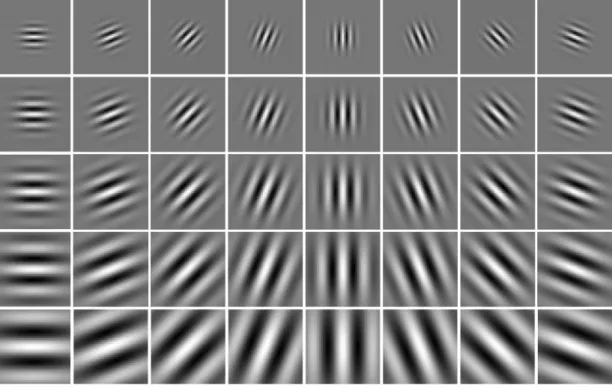
Figure 2.5: Example of Gabor filter bank

unknown class A class B class C class D class E

sample

(40)

CHAPTER 2. LITERATURE REVIEW 27

(41)

Chapter 3

Background Work

In the previous chapter, different texture descriptors were discussed. A texture descriptor or combination of descriptors are used to represent texture in numer-ical form, giving emphasis to unique properties of texture. However, a common problem is that texture patterns are often not uniform due to changes in orient-ation, scale, illumination and other factors. Consequently, grey scale invariance and rotation invariance along with computational complexity are key features for successful texture descriptors.

Local binary patterns (LBP) is a simple yet powerful grey scale invariant texture descriptor which encodes the neighbourhood into binary patterns. This chapter gives the detailed understanding of LBP and its variants.

3.1

Local Binary Patterns

LBP, first introduced in [78], represents a relatively simple yet powerful texture

descriptor describing the relationship of a pixel to its immediate neighbourhood.

In section 2.2.5, basic principle of LBP is given. Given below is an example for

LBP. B =    56 58 95 20 80 98 22 79 80   

is a 3×3 grey scale block from an image with centre pixel at location (i, j), then

the LBP code after application of Equations 2.32 and 2.33 is

   s(56−80) s(58−80) s(95−80) s(20−80) s(98−80) s(22−80) s(79−80) s(80−80)    Binary −−−−→    0×28 0×21 1×22 0×27 ₁_×₂3 0×26 ₀_×₂5 ₁_×₂4    LBP(8,1) −−−−−→28 28

(42)

CHAPTER 3. BACKGROUND WORK 29

3.2

Circular local binary patterns (LBP

cir_P,R

)

In the above procedure, the eight neighbourhood of each pixel are utilised. Clearly,

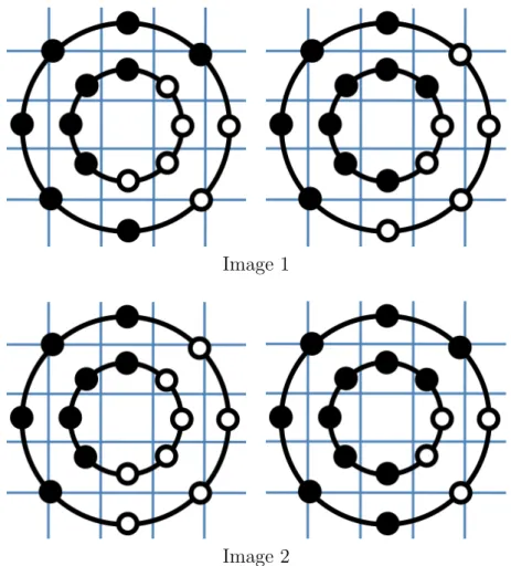
four of these neighbours are at different distance (√2) than the other four. To

compensate for this, a circular neighbourhood can be defined [79] as shown in

Fig-ure3.1where locations that do not fall exactly at the centre of a pixel are obtained

through interpolation. A circular symmetric neighbourhood defined by R and P

can be employed on which LBPs are calculated. Here,Rdefines the distance of the

neighbours to the centre whileP gives the number of samples at that distance that

are employed as neighbours. For centre pixel gc, the coordinates of neighbouring

pixelsgp, if p= 1,2, . . . , P are given by (−Rsin(2πp/P), Rcos(2πp/P)).

Figure 3.1: Square (left) vs. circular (right) LBP neighbourhood.

3.3

LBP Mappings

In [79] three mappings for LBP are proposed: rotation invariant, uniform and

rotation invariant uniform LBP. The rotation invariant mapping not only useful to reduce the feature length but also work exceptionally well on rotated texture data, giving rotation invariant texture description. Similarly, uniform mapping also reduces the feature length of LBP.

3.3.1

Rotation Invariant LBP (LBP

ri_P,R

)

If a texture is rotated essentially the patterns (that is the 0s and 1s around the

centre pixel) rotate with respect to the centre as illustrated in Figure 3.2 [79].

Rotation invariance of LBP, LBPri

P,R, is easy to obtain by considering the unique

minimum value of the binary patterns which is obtained by shifting the binary structure so as to end up with a sequence of a maximal number of 0s at the beginning. Mathematically, it is given as

(43)

CHAPTER 3. BACKGROUND WORK 30

Figure 3.2: LBP pattern and 90-degree rotated LBP pattern.

where ROR(x, i) performs a circular bit-wise right shift on the P bit number. In

Figure 3.2, if 1 is represented by black and 0 is represented by white, then the

texture before rotation gives pattern (10100111) and after rotation (10011110).

However, after applying LBPri_{, both images result in the same pattern (00111101).}

For eight neighbours, there are 36 rotation invariant LBP codes.

3.3.2

Uniform LBP (LBP

u2_P,R

)

Certain binary patterns are fundamental properties of texture and sometimes their

frequency exceeds 90%. These patterns are calleduniform, leading to LBPu2

P,R, and

are defined by a uniformity measure which corresponds to a spatial transition (i.e.

changes from 0 to 1 and vice versa) [79]. For example, in Figure 3.3, the image

on the left shows four changes and is hence considered as non-uniform while the image on the right has the uniformity index of two and is hence considered as the uniform pattern. The patterns with uniformity measure 2 are given by

LBP_P,Rriu2 =    PP−1 p=0 s(gp−gc) if U(LBPP,R)≤2 P + 1 otherwise (3.2) where U(LBPP,R) =|s(gp−gc)−s(g0−gc)| + P−1 X p=1 |s(gp−gc)−s(gp−1−gc)|

3.3.3

Rotation Invariant Uniform LBP (LBP

riu2_P,R

)

Clearly, rotation invariance uniform mapping can be achieved in the same way as above. For this both rotation invariant and uniform mapping are performed. For eight neighbours there are nine rotation invariant uniform LBP codes, two

(44)

CHAPTER 3. BACKGROUND WORK 31

as shown in Figure 3.4. While LBP generates 256 patterns for 8-neighbourhood,

LBPri _{generates 36 patterns, LBP}u2 _{generates 58 uniform patterns and LBP}riu2

results in 9 patterns for the same neighbourhood. In case of uniform and rotation invariant uniform patterns, all non-uniformed patterns are summarised into one bin for texture description.

3.4

Multi-scale LBP

By defining several radii around a pixel, multiple concentric neighbourhood LBP

codes can be extracted as illustrated in Figure 3.5. To capture LBP feature at

different scales, only the radius has to change. A large radius also allows to capture more neighbouring pixels, however that means more LBP patterns and thus finally the more feature length. Thus, LBP histograms corresponding to different radii are simply concatenated and used as texture features.

3.5

LBP Variants

It is clearly observed that LBP are simple texture descriptors, further to this various forms of LBP (LBP variants) are reported to boost the performance of LBP. In this section, different LBP variants are discussed.

3.5.1

Co-occurrence of Adjacent LBP (CoA-LBP)

In [75, 76], co-occurrence of adjacent LBP is proposed to preserve the spatial

re-lation between adjacent LBPs. In the proposed method the number of possible combinations will be significantly higher and hence auto-correlation matrix is pro-posed to calculate the co-occurrence of LBP. To reduce the number of LBPs two configurations are proposed: patterns derived only with horizontal and vertical pixels (LBP(+)) and the patterns derived by diagonal pixel (LBP(-)). Then the

correlation matrix is calculated by considering Np ×Np auto-correlation matrix

defined by following equation.

H(a) =X

r∈I

f(r)f(r+a)T (3.3)

where a is the displacement vector from the reference LBP to its neighbour

LBP. The element Hi,j(a) indicates the number of pairs of adjacent LBPi and

LBPj. In our experiments we extracted LBP at radius 1 and a is set to 1 pixel to

the right. Further, LBPs are generated at vertical and horizontal pixels to central pixel.

Multi-dimensional local binary pattern texture descriptors and their application for medical image analysis