Detection and tracking of Mmoving objects using stereo vision cameras

(1)

Thesis presented in partial fulfilment of the requirements for the

degree of Master of Engineering (Electronic) in the Faculty of

Engineering at Stellenbosch University

Author:

CE Roelofse

Supervisor:

Dr CE van Daalen

Department of Electrical and Electronic Engineering

Faculty of Engineering

Stellenbosch University

March, 2018

(2)

Plagiaatverklaring /

Plagiarism Declaration

1. Plagiaat is die oorneem en gebruik van die idees, materiaal en ander intellektuele eiendom van ander persone asof dit jou eie werk is.

Plagiarism is the use of ideas, material and other intellectual property of another’s work and to present is as my own.

2. Ek erken dat die pleeg van plagiaat ’n strafbare oortreding is aangesien dit ’n vorm van diefstal is.

I agree that plagiarism is a punishable offence because it constitutes theft.

3. Dienooreenkomstig is alle aanhalings en bydraes vanuit enige bron (ingesluit die internet) volledig verwys (erken). Ek erken dat die woordelikse aanhaal van teks sonder aanhalingstekens (selfs al word die bron volledig erken) plagiaat is.

Accordingly all quotations and contributions from any source whatsoever (including the inter-net) have been cited fully. I understand that the reproduction of text without quotation marks (even when the source is cited) is plagiarism.

4. Ek verklaar dat die werk in hierdie skryfstuk vervat, behalwe waar anders aangedui, my eie oor-spronklike werk is en dat ek dit nie vantevore in die geheel of gedeeltelik ingehandig het vir bepunting in hierdie module/werkstuk of ’n ander module/werkstuk nie.

I declare that the work contained in this assignment, except where otherwise stated, is my origi-nal work and that I have not previously (in its entirety or in part) submitted it for grading in this module/assignment or another module/assignment.

i March 2018

(3)

A

BSTRACT

Detection and tracking of moving objects (DATMO) is one of the core components nec-essary for autonomous navigation of a robot. The robot requires measurements of its envi-ronment, and uses these measurements to construct a representation of the dynamic objects in its environment. Once dynamic objects have been detected, the robot can use their locations and movement for autonomous functionality such as navigation, or collision prediction and avoidance. Of particular interest are vision-based sensors such as cameras, due to the amount of information they give about the environment. However, the amount of information causes difficulty regarding the interpretation and workable utilisation of the information.

This thesis outlines a systematic approach for robust estimation of states for DATMO using stereo vision cameras. The mathematical basis of the camera geometry is derived. These include the camera projection transform, camera parameters, and epipolar geometry. Image-features are obtained from both the left and right cameras and are matched. These matched image-feature pairs are triangulated to form 3D measurements of the moving objects in the robot’s environment. These 3D measurements are then used to filter the state estimates of the moving objects. Popular feature detection algorithms are expounded and investigated. ORB, KAZE, and A-KAZE are chosen for implementation and comparison. Factors pertaining to feature detection and matching, such as subpixel accuracy and matching strength, are weighed in light of a desired robust implementation.

The data association problem, that is which objects in the environment caused which mea-surements, is addressed. Methods used to address the problem, such as global nearest neigh-bour, probabilistic data association, and multiple hypothesis tracking (MHT), are examined. A multiple hypothesis tracking solution that uses Bayesian statistics is used in order to reli-ably associate measurements to objects in the robot’s environment. Necessary approximations to the MHT approach are made and justified. The approximations result in a first-order ap-proximation and a Gaussian mixture density description. The issue of unbounded associations is addressed and managed with techniques that remove, approximate, or prevent unnecessary state estimates.

Algorithms are tested using the KITTI dataset in Python. LiDAR is used to evaluate the re-sults of the algorithm. The computational cost of the algorithm is the biggest issue highlighted by the results. This is due to the complexity of the multiple hypothesis tracking solution and the large number of image-features used to ensure robust and reliable functionality. The re-sults of the thesis demonstrate that there is philosophical conflict between the requirement of robust estimation on the filtering side, and the large number of measurements required from camera images. The complexity increases with the number of measurements, but many mea-surements are needed in order to provide a reliable representation of the environment from camera images.

(4)

U

ITTREKSEL

Deteksie en volging van bewegende voorwerpe (DATMO) is een van die kernkomponente wat nodig is vir outonome navigasie van ’n robot. Die robot benodig metings van die ing en gebruik hierdie metings om ’n voorstelling van die dinamiese voorwerpe in sy omgew-ing te maak. Sodra dinamiese voorwerpe gevolg is, kan die robot hul posisies en bewegomgew-ing gebruik vir outonome funksies soos navigasie, of botsing-voorspelling en vermyding. Van belang is visie-gebaseerde sensors soos kameras, gegee die hoeveelheid inligting wat hulle beskikbaar maak oor omgewing. Die hoeveelheid inligting veroorsaak egter probleme met betrekking tot die interpretasie en werkbare benutting van die inligting.

Hierdie thesis beskryf ’n sistematiese benadering vir robuuste afskatting van toestande vir DATMO deur gebruik te maak van stereo-visie kameras. Die wiskundige basis van die kamera geometrie word afgelei. Dit sluit in die kamera projeksie transformasie, kamera parameters en epipolêre geometrie. Image-features word ontdek uit beide die linker en regter kameras en word geassosieer met mekaar. Hierdie geassosieerde image-feature-pare word gebruik om 3D-metings van die bewegende voorwerpe in die robot se omgewing te kry. Hierdie 3D-3D-metings word dan gebruik om die toestandafskattings van die bewegende voorwerpe te filter. Die mees populêre feature algoritmes word uiteengesit en ondersoek. ORB, KAZE en A-KAZE word gekies vir implementering en vergelyking. Faktore wat verband hou met feature-opsporing en assosiasie, soos subpixel-akkuraatheid en assosiasie betroubaarheid, word geweeg in die lig van die verlangde robuuste implementering.

Die data-assosiasie probleem, dit wil sê watter voorwerpe in die omgewing veroorsaak watter metings, word aangespreek. Metodes wat gebruik word om die probleem aan te spreek word ondersoek. ’n MHT oplossing wat Bayesiese statistieke gebruik, word gebruik om met-ings betroubaar te assosieer met voorwerpe in die robot se omgewing. Noodsaaklike be-naderings tot die MHT-benadering word gemaak en geregverdig, wat lei tot ’n eerste-orde benadering en ’n Gaussiese mengsel digtheidsbeskrywing. Die probleem van oneindige met-ing assosiasies word aangespreek met tegnieke wat onnodige toestandafskattmet-ings verwyder, benader of voorkom.

Algoritmes word getoets met behulp van die KITTI datastel in Python. LiDAR is gebruik om die resultate van die algoritme te evalueer. Die berekeningskoste van die algoritme is die grootste probleem wat deur die resultate uitgelig word. Dit is as gevolg van die kompleksiteit van die MHT oplossing en die groot aantal image-features wat gebruik word om robuuste en betroubare funksionaliteit te verseker. Die resultate van die thesis wys dat daar filosofiese kon-flik is tussen die vereiste van robuuste afskatting op die filterkant en die groot aantal metings wat van kamerabeelde vereis word. Die kompleksiteit neem toe met die aantal metings, maar baie metings is benodig om ’n betroubare voorstelling van die omgewing uit kamerabeelde te verseker.

(5)

IST OF

F

IGURES

1.1 Bayesian statistics example . . . 3

1.2 SLAM bayes net . . . 4

1.3 DATMO bayes net . . . 5

1.4 Simple projection . . . 7

2.1 Pinhole model . . . 10

2.2 Pinhole segmentation . . . 10

2.3 Epipolar geometry . . . 14

2.4 Epipolar geometry rectified . . . 15

2.5 Stereo geometry . . . 17

2.6 Harris eigenvalue plot . . . 20

2.7 Shi-Tomasi eigenvalue plot . . . 21

2.8 Laplacian of Gaussian . . . 22

2.9 Gaussian scale space . . . 23

2.10 SIFT descriptor . . . 25

2.11 Box filter approximation . . . 26

2.12 Integral image . . . 27

2.13 Haar wavelets . . . 28

2.14 SURF orientation . . . 29

2.15 Nonlinear diffusion . . . 30

2.16 FAST detection . . . 33

2.17 Markov bayes net . . . 39

2.18 GNN gates . . . 49 2.19 JPDA combinations . . . 53 3.1 Unfiltered disparity . . . 64 3.2 Filtered disparity . . . 64 3.3 Diagram overview . . . 66 4.1 ORB features . . . 67 4.2 KAZE features . . . 68 vii

(9)

4.4 Grid approach . . . 69 4.5 Feature matches . . . 70 4.6 Nonlinear triangulation . . . 72 4.7 Triangulation samples . . . 73 5.1 Spooky effect . . . 81 5.2 PHD clutter . . . 82 5.3 IMU samples . . . 84 6.1 MHT association tree . . . 85 6.2 Gating measurements . . . 88 7.1 KITTI setup . . . 93

7.2 LiDAR projected points . . . 93

7.3 Annotated image . . . 93

7.4 Annotated LiDAR . . . 94

7.5 Chi squared distributions . . . 95

7.6 Distribution in image . . . 97

7.7 Accuracy testing . . . 98

7.8 Chi squared result . . . 99

7.9 Extent and spread . . . 101

(10)

L

IST OF

TABLES

2.1 Table of feature comparison . . . 38

7.1 Table of KL divergence . . . 103

7.2 Missed detections . . . 104

7.3 Table of computational cost . . . 104

7.4 Table of timing allocation . . . 106

(11)

N

OMENCLATURE

This section contains abbreviations and mathematical notations used in this thesis.

1. Abbreviations

A-KAZE Accelerated KAZE

AOS Additive Operator Splitting

BRIEF Binary Robust Independent Elementary Features

CPHD Cardinalised-PHD

DATMO Detection And Tracking of Moving Objects

div Divergence

DoG Difference of Gaussian

EKF Extended Kalman Filter

FAST Features from Accelerated Segment Test

FED Fast Explicit Diffusion

GM-PHD aussian Mixture Probability Hypothesis Density

GM Gaussian Mixture

GNN Global Nearest Neighbour

GPU Graphics Processing Unit

IMU Inertial Measurement Unit

IW Inverse Wishart

(12)

KF Kalman Filter

KL Kullback-Leibler

LDB Local Difference Binary

LoG Laplacian of Gaussian

M-LDB Modified-Local Difference Binary

MHT Multiple Hypothesis Tracking

MTT Multiple Target Tracking

oFAST Oriented FAST

ORB Oriented FAST and Rotated BRIEF

PDA Probabilistic Data Association

PHD Probability Hypothesis Density

rBRIEF Rotated BRIEF

RFS Random Finite Set

RTK Real Time Kinematic

SIFT Scale-Invariant Feature Transform

SLAM Simultaneous Localisation And Mapping

SURF Speeded-Up Robust Features

UKF Unscented Kalman Filter

(13)

2. Mathematical Notation

a Scalar

a Vector

A Matrix

xk Vector at timestepk

x1:k Collection of vectors from timestep 1 to timestepk

X_k Set at timestepk, unless defined otherwise

X_1:_k Set of collected sets from timestep 1 to timestepk

G(·) Vector function

µ

µµ Gaussian mean

ΣΣΣ Gaussian covariance

N (·, ·) Define Gaussian distribution

p0 Homogeneous coordinate of pixel position

p Homogeneous coordinate of state space position

0 Vector of zeros

I Identity matrix

IKL(·||·) KL divergence

D2_MAL Squared Mahalanobis distance

χ2(k) Chi squared distribution withkdegrees of freedom

e· Merging approximation of quantities p(x) Probability density function ofx

(14)

1.

I

NTRODUCTION

In the last 50 years, academia and business industry have been working toward realising a more autonomous robotic future. Robotics itself have been widely utilised and have even taken over certain industries. A prominent example of such an industry is the manufacturing industry, where robotics is extremely useful given the repetitive mundane nature of tasks. However, attempting to realise reliable autonomous robots has proven to be difficult and a more complex problem than anticipated. These robots need to function independent of human assistance in a dynamically changing environment with moving objects in the environment. Navigating independently in such an unstructured dynamic environment requires methodologies that are robust and reliable. The problem is further complicated by the ego (self) motion of the robot. All measurements are obtained at different positions in the environment and relating these measurements to one another requires the location of the robot to be known. Autonomous functionality requires robust techniques for sensor data filtering and reliable logic that governs autonomous decision making.

1.1 Autonomous Functionality

Sensor data is required in order to give a computer system an abstracted representation of its environment. This representation is abstracted by nature since it is not a direct exhaustive representation of the environment, and therefore reductionistic. This representation needs to be interpretable in such a way as to yield useful understanding of what is present in the envi-ronment, and therefore be functional, that is facilitate interaction with the environment. This interaction could be a range of desired applications such as navigating through the environ-ment, or reliably predicting what might change in the environment. Autonomous functionality is a complex problem given the difficulty of robustly and reliably functioning in a dynamically changing environment.

Cameras have been of particular interest as sensors given the amount of data available in vision-based sensors. However, they have posed difficult challenges. One of the difficul-ties of processing vision-based data is that it is not self-evident how to process and interpret vision-based data in a way that results in a useful representation of the environment. Instead

(15)

of making direct state space data available, such as position and velocity, the appearance of things in the environment is instead available. The other issue is the computational burden of interpreting and processing the amount of data present. Regardless of the difficulties as-sociated with cameras, they are still of interest for the purpose of autonomous functionality given the amount of information present. In fact, the ever-increasing capabilities and advance-ments of processors have gradually made vision-based sensors more relevant and viable, and continue to do so.

1.2 Probabilistic Robotics: Bayesian Statistics

The required usable representation needs to describe the states of moving objects of interest, such as their position and velocity. If these states are known, then they can be used to facilitate autonomous functionality. The robot could use the information to predicate where moving objects would be in the future, and navigate accordingly. However, the issues of sensor noise and robot localisation error result in uncertainty in the resultant states of moving objects. This uncertainty reduces the reliability of the environment’s representation. These issues are addressed with probabilistic techniques and the approach known as probabilistic robots.

The challenge of autonomous functionality is approached with probabilistic methods. These methods are used because they model the inherent uncertainty both in the environment and in the measurements of the environment. Probability density functions are used to characterise measurement, process, and state estimate uncertainty. These probabilistic representations can be used in a Bayesian framework to produce estimates of the hidden states of moving and stationary objects [68], along with the robot’s pose (position and orientation). These resultant estimates can be used to track moving objects and facilitate autonomous functionality. A Bayesian statistical approach is predicated on Bayes theorem [68] described by Equation 1.1, and can be derived using conditional distributions. This theorem is the basis of statistical inference. Given the prior distribution over random variablex, and the conditional distribution of the measurementzgivenx, the likelihood function p(z|x), the posterior distributionp(x|z)

can be determined.

Given the likelihood function p(z|x), prior distribution p(x), and the marginal distribution of the data p(z), the posterior distribution p(x|z)can be determined. The posterior distribution is proportional to the product of the likelihood function and the prior distribution since p(z)

functions as a normalisation constant, that is

p(x|z) = p(z|x)p(x)

p(z) ∝p(z|x)p(x). (1.1)

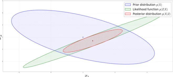
Figure 1.1 demonstrates a simple two-dimensionalx= [x₁, x₂]T example of Bayesian infer-ence, where the three ellipses represent one standard deviation contour plots of joint bivariant

(16)

Gaussian distributions over thex∈_R2_{space. The prior belief (blue) about} _x_{is updated with}

a measurement (green) and results in a posterior belief (red). The Bayesian statistical frame-work facilitates the inherit uncertainty, in measurements and states, in order to yield resultants that represent the degree of the robot’s certainty. Once moving objects’ states and measure-ments are represented by random variables, they can be cast into a Bayesian framework. The resultant distributions are then used to facilitate autonomous functionality, but with the added benefit of having a measure of certainty about the environment that the robot is functioning in.

Figure 1.1: Two-dimensional joint Gaussian Bayesian inference example.

Applications of Bayesian Filtering: SLAM and DATMO

Two of the more popular design approaches that facilitate autonomous operation are SLAM (simultaneous localisation and mapping) and DATMO (detection and tracking of moving ob-jects). These frameworks, given the discussed inherent uncertainty, are approached and mod-elled with Bayesian statistics.

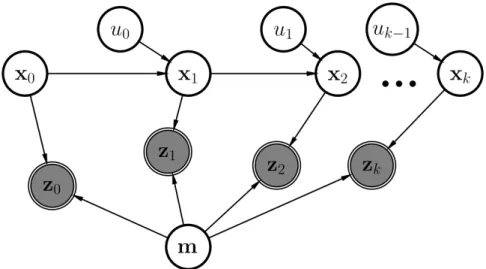
The objectives of SLAM are twofold [65], [66]. First a map estimate of the robot’s environ-ment is created. This map is created by using measureenviron-ments of stationary landmarks in the environment and the robot is localised with respect to the landmarks. Stationary landmarks are used to create the map due to their reliability as fixed points with little process noise or modelling error [75]. Moving objects have more relative uncertainty in their state estimates, and would cause increased uncertainty in the robot’s localisation. The second objective is to localise the robot (the robot’s pose) using the map estimate without the use of inertial sensors. Figure 1.2 shows a Bayesian network of the SLAM process. The network visually illustrates how different random variables cause or influence other random variables with arrows indi-cating the nature of causation. x_k indicates the robot pose, z_k the measurements, and mthe

(17)

map, which consists of the estimated landmark locations. u_k denotes the robot commands that influence the next states of the robot. The prediction-update posterior result derived from Bayes’ rule of conditional distributions is expressed by [76]

p(x_k,m|Z_k,U_k₋₁)∝p(zk|xk,m) Z

p(x_k|x_k₋₁,u_k₋₁)p(x_k₋₁,m|Z_k₋₁,U_k₋₂)dx_k₋₁. (1.2) The hidden map mand states xk are estimated simultaneously with the assumption that the map is static, that is the landmarks constituting the map are stationary. Capitalised letters indicate the collection of all of its lower case counterparts from k=0 up until the current subscriptZ_k={z0, z1, ..., zk}. The resultant posteriors can be used to facilitate autonomous functionality, given that the robot has an understand of where it is in the environment.

Figure 1.2: Bayesian network for SLAM. Shaded nodes indicating observed states and non-shaded nodes indicating hidden states. Subscripts indicating the discrete time instance.

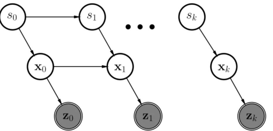
The objective of DATMO is simply detecting and tracking moving objects and can be used in a variety of frameworks, including or excluding inertial sensors. DATMO can be used in conjunction with SLAM, and can be advantageous for the purposes of SLAM, given that DATMO can determine which objects are dynamic and therefore function as a form of out-lier detection [74]. By determining which tracked objects are dynamic, the SLAM process can exclude dynamic tracked targets from candidacy as stationary SLAM landmarks. Petro-vskaya has stated that DATMO can be classified into three different frameworks, traditional, model-based, and grid based DATMO [56]. Traditional DATMO focuses on estimating states in a Bayesian context with data segmentation and association techniques, that is determining which objects in the environment caused which measurements. Model-based DATMO per-forms inference directly on the sensor measurements without segmentation and association. Grid based DATMO constructs a grid representation of the dynamic environment of the robot.

(18)

Traditional DATMO is of interest due to its general Bayesian formulation and state inference in the state space.

Figure 1.3: Bayesian network for DATMO.s_k indicates a discretely distributed random vari-able and denotes the motion model of a moving object, which governs the evolution of its states.

Figure 1.3 depicts a Bayesian network for traditional DATMO. The depiction deals with the issue of both state estimation and dynamic model estimation. xkdenotes the states of tracked moving objects, andzkthe measurements of the states. Any given moving object could be op-erating under different dynamics that govern its future states, for example a constant velocity model or a constant acceleration model. The depicted formulation estimates these dynamics and uses the dynamic model estimation to estimate the states. The estimation of model dy-namics could increase the propagation accuracy of states and as a result increase the accuracy of the state estimates. Equation 1.3 describes the estimation of the state and motion mode of a moving object [76], that is

p(xk,sk|Zk) =p(xk|sk,Zk)p(sk|Zk). (1.3) Using Bayes’ rule, the problem can be divided into astate inference p(xk|sk,Zk)problem and amodel learning p(s_k|Z_k)problem [76]. The estimated model is used in the state inference process. In order to alleviate some of the computational burden, amodel selectionlearning ap-proach is typically used. Model selection chooses from a finite set of possible model dynamics modelled by the discrete random variables_k.

This section illustrates how the formulation of a state estimation problem using Bayesian statistic can be used. This formulation models the inherit uncertainty in the process of state estimation. Resultant state estimates of tracked moving objects can be used to facilitate au-tonomous functionality such as path planning and collision prediction. SLAM was addressed in order to illustrate how DATMO can contribute to SLAM landmark candidacy filtering, and therefore be appropriated for more than the standard moving object tracking.

(19)

1.3 Cameras as Sensors: Approach and Limitations

Cameras are used for DATMO in a variety of configurations and use different image processing techniques. Cameras can be configured into mono, stereo, or multi-vision set-up. Stereo or multi-vision allows for depth information to be extracted, while mono-vision does not. Depth information for mono-vision can be obtained if the camera moves, assuming a relatively static environment, creating a synthetic baseline. Depth estimation accuracy (for any configuration) decreases as the baseline distance between cameras decrease, and decreases as the true depth of objects increase. Obtaining depth information of objects is required in order to estimate the states of an object or landmark in the environment.

In order for depth estimates to be obtained, corresponding points in at least two different camera images, with overlapping field of view of the scene, need to be found and correctly matched. Chosen points are referred to asimage features. Typically an image feature consists of two things. First, akeypoint which is a location in the image plane with an orientation. Second, adescriptor which describes the appearance of the feature and is typically a func-tion of the local gradients around the keypoint locafunc-tion. Salient pixel gradient and intensity characteristics are popular for interest point inspection, that is interest for feature usage. Inter-est points are inspected for feature candidacy due to their repeatability, that is the frequency with which they appear in multiple images over time. Their repeatability is attributed to their salient pixel gradient and intensity characteristics. Feature descriptors, describing points in the environment, are matched between two images at a given synchronised time, and as a result the depth of the point into the scene can be determined. The accuracy with which the depth can be determined is dependent on the accuracy with which a feature keypoint is localised. Given that an image has a finite resolution, subpixel localisation techniques are typically used to obtain more accurate feature keypoint locations.

During the feature matching phase, using the feature descriptors, there is always a chance that an incorrect correspondence can be made, that is a mismatched feature pair which leads to an incorrect representation of the environment. This issue can be mitigated to a certain extent by using a variety of techniques. Some of these techniques include using thresholds for the similarity of a potential match. Others include only using correspondences that are found to match both ways between image pairs, that is matching pairs that are found both when starting with the left image and search for matches in the right image, and vice versa. The geometrical constraints introduced by compensating for the pose of the individual cameras are also used to constrain the missed match issue.

Figure 1.4 is a simple representation of feature points in the world projected into the camera image plane. The dimensionality is reduced and only objects in the field of view of the camera are detected. These feature points are localised and described for the purpose of tracking and

(20)

matching between different cameras. These matches are triangulated in the environment and used in a Bayesian inference filtering framework in order to obtain estimates of the states of the detected objects.

Figure 1.4: Camera projection from the 3D world, that is state space, to the image plane, that is measurement space. Image reproduced with permission from Rougier [2].

1.4 Thesis Scope

This thesis focuses on robustly and reliably obtaining and processing (filtering) measurements of moving objects using stereo vision cameras, in order to track and represent the activity present in the environment. The resultant representation could be used to facilitate a number of autonomous functionality. Various techniques used to generate measurements from camera sensor data is inspected with the focus on feature detection. The reliability of these tech-niques is of interest. Filtering these measurements in order to yield state estimates is done in a Bayesian filtering framework, which models the inherit uncertainty, as stated. The resultant state estimates give a measure of the reliability of these state estimate locations. The issue of determining which moving object generated which measurement, mentioned only briefly, is explored. This measurement causation problem is solved by determining which technique that addresses this issue is the most robust to error. Different feature detection techniques are used and compared in order to inspect their reliability as robust methods for DATMO.

(21)

2.

L

ITERATURE REVIEW

This section contains a literature review about topics that relate to the application of tracking dynamics objects with cameras. These include camera modelling, stereo geometry, feature detection, measurement filtering, and data association strategies. The model used to describe the transformation of a 3D point to a 2D point in the image plane is derived. Once the cam-era model for an individual camcam-era is derived, stereo vision geometry is expounded. This geometry is ultimately used for the purposes of determining the position of a 3D point in the environment, given a matched pair of features from the two stereo cameras. Determining the location of this 3D point is required in order to track a moving point in the environment.

Various feature detection algorithms are explored and investigated. Once points are found, they are matched using feature descriptors. The match can then be triangulated into the envi-ronment, resulting in the 3D state space location of the detected point. The issue of determin-ing which measurements where caused by which movdetermin-ing objects needs to be addressed. The most popular techniques are evaluated and inspected.

2.1 Camera Model

Using cameras as sensors in tracking applications requires a mathematical foundation. This foundation should describe the mathematical transform that occurs when an object is within a camera’s field of view. This transform is from the state space (the world) to the measurement space (the camera’s image plane). In this section the mathematical model of a single camera is first derived, and then extended to stereo vision.

2.1.1 Pinhole Camera Model

This subsection focuses on the fundamentals of the popularpinhole camera model[58]. This foundation is canonically used in literature relating to any work that uses the camera projection transform. All camera parameters that are relevant to the required transform are modelled using the pinhole camera model as the foundation. After the pinhole camera model has been covered, it will be used to derive the transform of a 3D point in state space to its image

(22)

projected point in the camera, the measurement space. This transform is a function of the intrinsic camera parameters.

Intrinsic Camera Parameters

The pinhole camera models the aperture (small opening through which light passes) of the camera as a single point, and as a result the only light that enters the camera is light that passes through this pinhole point, called theoptical centre. The pinhole modelling choice is an apt approach given that the aperture of a camera is necessarily small, since larger aperture sizes can result in more image blurring. This blurring is due to the fact that light from the same 3D point would intersect the image plane at multiple points. These intersection points increase as the aperture size increases. Using the pinhole model, light passes through the optical centre and creates a vertically inverted image on theimage planea distance off behind the optical centre. This distancef is called thefocal length. Analogously, an image plane a distancef in front of the camera (instead of behind) can conceptually be used. This image plane in front of the camera produces a non-inverted image. Both Figures 2.1 and 1.4 depict a visualisation of an image plane in front of the optical centre.

Figure 2.1 depicts the geometry used to derive the camera transformation model from the pinhole camera model [58]. The 3D Cartesian axis denotes the position of the camera with the origin being the optical centre. Y_C point downward below the camera. The optical axis corresponds to the Z_C axis and points in the direction that the camera is facing, that is the camera lens opening. This axis is referred to as the camera coordinate system.

A pointp∈_R3_{described in camera coordinates is projected onto the image plane and}

conse-quentially creates a pointp0∈_R2_{. Notice how the projection line (which is the light ray) in}

Figure 2.1 is projected toward the optical centre (pinhole), and the intersection of the projec-tion line and the image plane creates pointp0a distancef from the optical centre. The camera projection transform results in a reduction of dimensions, that is

p0=G(p), G: R3→R2. (2.1)

As a result, in the mono vision case, the full 3D state cannot be recovered if one starts with the projected pointp0, unless multiple cameras are used.

The transform G can be derived using simple geometry of similar triangles that describes proportional triangle side lengths. Figure 2.2 is a two dimensional slice of Figure 2.1’s model along theY_C-axis, that is Figure 2.2 is in the X_CZ_C-plane. x_p is the projection’s horizontal position (in pixels) in the image plane measured from the principal pointcin Figure 2.1.

(23)

Figure 2.1: Pinhole camera projection model. cis the principal point where the optical axis intersects with the image plane. The figure is based on a diagram created by Botha [33].

Figure 2.2:X_CZ_C-plane of camera projection model. p0is located in the image plane, denoted by the pink bar.

The desired transform can be expressed as

xp f = x z ⇒ xp= f x z. (2.2)

Equation 2.2 is derived using proportional triangle sides withf in units of pixels. Similarly,

y_p f = y z ⇒ yp= f y z (2.3)

can be derived using aY_CZ_C-plane section,y_pbeing the projection’s vertical position (in pixels) in the image plane.

(24)

zp0=    f 0 0 0 0 f 0 0 0 0 1 0   p, (2.4)

using homogeneous coordinates withp0= [x_p, y_p, 1]T andp= [x, y, z, 1]T. This expression allows for the transform to be expressed in matrix form, which is not possible using Cartesian coordinates since the formulation does not allow for product and division operations. How-ever, using homogeneous coordinates results in a matrix notation withz6=0, the depth of the 3D point, which scales the resultant projection pointp0, as expressed in Equation 2.4.

At this point the transform of a 3D point in state space to measurement space has been derived. This derivation is facilitated by the pinhole camera model. Next some of the physical camera parameters that influence the transform will looked at and modelled. These parameters need to be modelled in order to result in an accurate projection transforms that is representative of the physical projection process.

The focal length f was the first of the mentioned parameters and is used to derive the projection transform. These parameters form part of the pinhole camera model. Other parameters include the principal point location, the non-square factors, and the skewed pixel factor. The principal pointc= (c_x, c_y)is the point where the optical axis intersects the image plane. This point is not necessarily at the origin, the middle of the image plane, but can be offset. This offset needs to be modelled and accounted for. The non-square factorsα and β are used to compensate

for pixels which are vertically or horizontally elongated (as rectangles). The skewed factorτ

is used to compensate for any vertically skew (slanting) aligned pixel columns. Radial lens distortion can also be modelled and compensated for as well, but is neglected in this section. Radial distortion does not form part of pinhole camera model, but is required to transform an image of an actual camera to something representing the pinhole camera model. Adding these intrinsic factors to Equation 2.4 results in

zp0=    αf τ cx 0 0 βf cy 0 0 0 1 0   p= KI 0 p; (2.5)

KI is referred to as the intrinsic camera matrix [29], [40]. These parameters are typically found using self-calibration methods such as those implemented by OpenCV. A variant of Zhang’s [82] method of planar calibration is implemented in OpenCV. This method uses a specific planar pattern with known dimensions and with known feature point correspondence, that is features from the specific pattern. The plane and its features are observed by the camera from different perspectives which are used to determine the parameters expressed in Equation 2.5. A certain minimum number of perspectives are required, but usually more are used,

(25)

resulting in an overdetermined problem. This is done in order to result in estimates that are more robust to noise.

External Camera Parameters

The external parameters of the camera can be characterised by the pose of the camera’s body axis relative to an inertial (or world) axis. An orthonormal 3x3 rotation matrix RW and a translation vector tW, describing the pose of the inertial axis origin in camera coordinates, can be used to transform a point described in the inertial coordinate systemp_W to a camera coordinate systemp (Equation 2.6). Therefore, if a 3D point is described in any coordinate system and the pose of this coordinate system relative to the camera is known, then the 2D projection point can be determined. Similarly, rotation matrixRC and a translation vectortC, describing the pose of the camera coordinate system origin relative to an inertial coordinate system, can be used to transform a point described in the camera coordinate systempto inertial coordinate systemp_W, that is

p= " RW tW 0T 1 # p_W & p_W = " RC tC 0T 1 # p. (2.6)

This transformation of coordinate systems is required since the camera projection transform is derived by assuming a camera coordinate system representation, with 3D points described in the camera coordinate system. However, when dealing with implementation,RW andtW are not available, but insteadRC and tC, the camera or robot’s pose, are available by using an inertial sensor such as an IMU. Therefore, theextrinsic camera matrix KE is derived and described in terms ofRC andtC, since they are typically known. Looking at the descriptions in Equation 2.6, it follows that

" RW tW 0T 1 # = " RC tC 0T 1 #−1 , (2.7)

and decoupling the pose into translation and rotation matrices results in

= "" I t_C 0T 1 #" R_C 0 0T 1 ##−1 = " R_C 0 0T 1 #−1" I t_C 0T 1 #−1 , (2.8)

(26)

withIdenoting the identity matrix, which simplifies [9] to = " R_CT 0 0T 1 #" I −t_C 0T 1 # = " RT_C −RT_Ct_C 0T 1 # =KE. (2.9)

Factoring in the intrinsic camera matrix, as stated in this subsection results in

zp0= KI 0 p. (2.10)

Expandingp to be a function of a point described by any coordinate system, using Equation 2.6, results in = KI 0 " R_W t_W 0T 1 # p_W. (2.11)

Substituting Equation 2.9 into Equation 2.11 results in

= KI 0 " RT C −RCTtC 0T 1 # p_W (2.12) and zp0= KI 0 KE p_W. (2.13)

Equation 2.13 describes the camera projection transform in homogeneous coordinates, includ-ing intrinsic and extrinsic camera parameters [9]. Usinclud-ing this formulation requires an estima-tion of the intrinsic parameters and requires an inertial senor to obtain the extrinsic parameters. This formulation is for the mono vision case. Estimating the states of a moving object in 3D a requires depth information, which in turn requires multiple perspectives of the moving object. As a result, the projection transform needs to be expanded to the stereo vision case.

2.1.2 Stereo Geometry and Rectification

In practice, stereo image pairs are not necessarily aligned, that is projected points in one image that correspond to the projected points of the same 3D point in the second image are not horizontally aligned. This is due to their relative individual poses. A process known as stereo rectification is used to compensate for the relative pose of the cameras. Stereo rectifying

(27)

images with an overlapping field of view results in easier feature match searches. Once the images are stereo rectified, all corresponding projected point matches are horizontally aligned and need to be searched for along horizontal lines.

Stereo Rectification

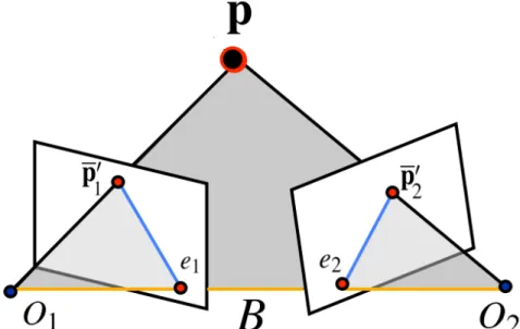
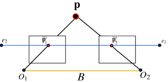
Figure 2.3 shows a stereo camera setup with optical centreso₁ and o₂. Pointp is projected too₁ando₂, resulting inp₁0 and p0₂. Optical centres are separated by baseline distanceB. e₁ ande₂are the points whereBintersects the image planes and are known asepipoles[43]. The lines in the image planes (blue lines) fromp0₁toe₁(first line) and fromp0₂toe₂(second line) are known asepipolar lines. The first epipolar line represents possible positions forp0₁ in the image plane, given a fixed corresponding pointp0₂. Aspmoves along thep−o₂line towardo₂, p0₁moves along the epipolar line toward the epipolee₁. The correct correspondence matching point is located along the epipolar line, and as a result a search for the match is constrained along the epipolar line. This constraint is called theepipolar constraint[54].

Figure 2.3: Stereo geometry displaying epipolar lines. A point is projected into two image planes, separated by baselineB, resulting in to projected points. These projection points are constrained along certain lines in the image planes. Image reproduced with permission from Savarese [1].

The process of rectification places the epipoles at infinity, and consequently the epipolar lines become parallel with the horizontal axis of the image planes. The image planes also become co-planar, situated in the same plane. The horizontal epipolar lines between the two images are aligned, placing each corresponding point at the same vertical position in the image planes, and along a horizontal line [1].

(28)

Figure 2.4 shows the result of rectification. Epipolar lines are horizontal and the epipoles are at infinity. The baseline intersects the shared plane in which the two image planes are now situated an infinite amount of time, that is the baseline lies within the plane. Corresponding points are located along the epipolar lines, which are now at the same vertical positions. This reduces the difficulty with which corresponding point matches need to be looked for. The resultant rectification is used in order to find image feature correspondences between rectified images. Practically, rectification is achieved by determining the pose of each camera relative to a planar surface with a known pattern and dimensions. Both cameras observe the planar surface with different poses. The known pattern produces strong feature responses with known correspondences between cameras. These correspondence matches between the two cameras of the same planar surface are used to determine the relative pose the cameras, and these poses are used to compensated for image alignment. Stereo rectification functions are also implemented in OpenCV.

Figure 2.4: Stereo geometry displaying horizontal epipolar lines after rectification. Image reproduced with permission from Savarese [1].

The process of feature detection still needs to be addressed, but before feature detection pro-cesses are addressed, the stereo projection transform needs to be determined. This transform describes how a matched feature pair transforms from state space to measurement space, and vice versa, the reverse being referred to astriangulation, since the 3D point is triangulated into the state space using the matched pair. If the reader recalls, this reverse operation is not possible in the mono vision case since the mono vision case results in a reduction of dimen-sions.

(29)

Stereo Geometry

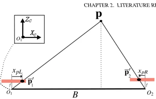
With images stereo rectified, the transform from 3D Cartesian camera coordinates, in meters, to image plane pixel positions, in pixels, can be derived. x_pL denotes the horizontal pixel position of p= [x, y, z]T’s projected position in the left image plane, and y_pL denotes the vertical pixel position ofp’s projected position in the left image plane. A four dimensional vector of a matched feature pair, [x_pL,y_pL,x_pR,y_pR], is reduced to a three dimensional vector, [x_pL,x_pR,y_p], given thaty_pL=y_pR=y_pafter stereo rectification. The transform can be derived using similar methods as the mono vision case.

Figure 2.5 is a XCZC plane section of a stereo vision camera setup, using pinhole camera models. The principal point offset is neglected in the figure. o1 ando2 are the optical centres

of the cameras. The origin of the Cartesian axis, describingp, is located ato1. The derivation

is approached by using geometry of similar triangles, two equations from the XCZC plane section depicted in Figure 2.5, and one equation from aYCZC plane section. The resulting equations are described by

x_pL= f x z +cx, (2.14) x_pR= f(x−B) z +cx, (2.15) and y_p= f y z +cy. (2.16)

The triangulation process describes the reverse of this transform, transforming a feature matched pair in the two image planes to a 3D position defined by

x= B(xpL−cx) xpL−xpR , (2.17) y= B(yp−cy) x_pL−x_pR , (2.18) and z= f B xpL−xpR . (2.19)

(30)

Figure 2.5: Stereo geometry,XCZC-plane of camera projection model. The 3D point is pro-jected into both the left and right stereo rectified cameras creating a corresponding match that can be triangulated back into the 3D space.

The triangulation equations can be used to determine the 3D position of a point in the en-vironment. This point could be of a moving object, and as a result can be used to track a point in the 3D space. These image-feature points are determined by using feature detection techniques. Once features are detected, their descriptors are matches between stereo rectified images. Once matched, the feature matched pair can be triangulated into the environment.

2.2 Feature Detection

The derived camera model and transforms provide the framework in which pairs of matched points can be triangulated into the 3D space and vice versa. However, how to process and interpret the images themselves in a way that results in reliable and robust points is a separate problem. Image feature detection is one of the more popular methods of using visual sensor measurements. Feature detection searches for salient gradient or intensity behaviour and in-spects them as interest points, that being interest for feature candidacy. Corner features are of interest due to their repeatability and distinctness, that is the relative reliability with which they will be appearing and be detectable over time.

These features consist of akeypointlocation, with an orientation, and adescriptordescribing the appearance of the feature. Descriptors are a function of the local gradients or intensi-ties around keypoints and are used to describe a feature in a distinctive manner. Features are merely points in images, that when matched can be triangulated to a 3D point in the environ-ment. As a result, they do not represent the full physical extent of moving objects. However, tracking a point located on a moving object is sufficient in order represent that there is in fact

(31)

a moving object present in the environment. Moving objects are assumed to be rigid, for ex-ample a vehicle, and therefore in most cases every point that could be tracked on the object would have the same velocity, given the rigid assumption. As a result, the assumption is that the velocity of a 3D point mass located on a moving object is representative of the movement and location of the object given the rigid assumption, but it is not representative of the ob-ject’s extent. Therefore, features can be used to track objects, even though they lack extent representation.

Desirable attributes of features are rotation invariance and scale invariance. If a descriptor is rotation and scale invariant, then the descriptor can be matched even if the scene or camera rotates (rotation), or if the camera moves closer or further away from the moving object (scale). Some of the most popular algorithms used to detect features from images include SIFT, SURF, KAZE, and FAST, which are, amongst others, expounded in this section.

2.2.1 Early Feature Detectors

This subsection investigates two of the early feature detectors that are used to find corner points in an image. These are not considered as candidates for the thesis, but contain critical techniques that are used by the more modern feature detectors.

Harris Corner Detector

The Harris corner detector is the one of the oldest means of finding feature points in an image. Corners in an image have large pixel intensity gradients in both the horizontalx and vertical ydirections. In order to detect these gradients, the differences of pixel intensities in a certain windowware inspected, as expressed by

E(x,y) =

∑

u

∑

v

w(u,v)[I(u+x,v+y)−I(u,v)]2. (2.20) The size of the corner in the image would determine how large the window would need to be. E(x,y)is the sum of the weighted square of pixel intensity differences in a given window. I(x,y)denotes the pixel intensity of a grey scale image at(x,y), andw(u,v)is a window function (box or Gaussian) that is swept over the image. The content in this subsection is reproduced from OpenCV documentation [6] and Derpanis’s paper on the Harris corner detector [27].

Equation 2.20 is simplified by approximating I(u+x,v+y) with a first-order Taylor series expansion, as described by

(32)

with the underlying assumption being that the windowing shifts are small. Ixand Iydenotes partial derivatives of imageI with respect to the variable indicated by their subscript. This assumption results in

E(x,y)≈

∑

u

∑

v

w(u,v)[I(u,v) +Ix(u,v)x+Iy(u,v)y−I(u,v)]2, (2.22) and can be further condensed to

E(x,y)≈

∑

u

∑

v

w(u,v)[Ix(u,v)x+Iy(u,v)y]2. (2.23)

Equation 2.23 can be written in matrix form as

E(x,y)≈hx y i M " x y # , (2.24) withMdefined as M=

∑

u

∑

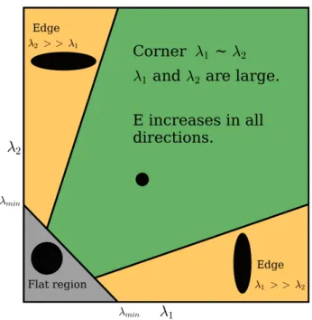
v w(u,v) " I2_x IxIy IxIy I2y # = " hI2_xi hIxIyi hIxIyi hI2yi # . (2.25)

Angled bracketsh·idenote averaging, which is caused by the summation and is a function of the type of window (weightings) used. The resulting matrix is referred to as theHarris matrix and its elements are thexandyderivatives of a patch (segment) of an image, isolated my means of a window function. In order to maximise the functionE(x,y), large variations in bothxand y are required, which can be evaluated by inspecting the Harris matrix’s eigenvalues, λ1,2.

Large eigenvalues indicate large deviations in the vector[x, y]T. Small eigenvalues indicate a planar (flat) region, that is a low gradient monochrome region. A single large eigenvalue indicates a single large gradient, an edge, and two large eigenvalues indicate a corner. The ratio of the two eigenvalues needs to be smaller than a certain threshold in order for the area to be regarded as a reliable corner.

Eigenvalue decomposition is computationally expensive and as a result

R=λ1λ2−k(λ1+λ2)2=|M| −kTrace2(M)>λmin (2.26) has been suggested by Derpanis [27], which is a function of the eigenvalues, but is computa-tionally more efficient. Rgives a measure of the ratio of the eigenvalues. The constantkhas been calculated empirically for typical applications (in the range of 0.05 – 0.15). As a result, the determinant and trace operations are used, instead of eigenvalue decomposition, and if the result is larger than a determined threshold the interest point is regarded as a reliable corner.

(33)

Figure 2.6: Eigenvalue classification illustration for Harris corner detector. This illustrates the classification of an inspected area as either being a plane (grey, small|R|), being an edge (orange,R< 0), or being a corner (green, large R). The ellipses are visual representations of the eigenvalue ratios. Large eigenvalues with small ratios are desirable.

The result of this classification process is a function of the Harris matrix’s eigenvalues. The classification process can be visually represented by Figure 2.6. The Harris corner detector as a stand-alone method is not scale invariant, and is not itself used as a feature detector since it does not build a feature descriptor. However, the methods used in this early interest point detector plays an important role in further developments.

Shi-Tomasi: Good Features to Track

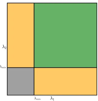
Shi and Tomasi, in good features to track [64], augmented Equation 2.26 resulting in

R=min(λ1,λ2)>λmin, (2.27)

and demonstrated that their adjustment yields a better threshold scoring function than Equation 2.26. Equation 2.27 simply states that bothλ1andλ2need to be larger than a certain threshold

λmin. Instead of determining a result that concerns itself with the ratio of the eigenvalues, both eigenvalues simply need to be larger than a specified threshold. This alteration can be visually represented by a similar eigenvalue plot depicted by Figure 2.7. Evidently, both Harris and Shi-Tomasi’s methods result in similar mapping regions as portrayed by Figures 2.6 and 2.7, with Shi-Tomasi’s method being a more reductionist approach, since it ignores some of the ratio complexity present in Derpanis’s derivation [27].

(34)

Figure 2.7: Eigenvalue classification illustration for Shi-Tomasi corner detector which is sim-pler than the Harris corner detector.

2.2.2 Modern feature detectors and formulations

While the early interest point detectors offer critical insight into feature detection strategies, they lack descriptors, and rotation and scale invariance. The modern feature detection tech-niques address these issues resulting in robust distinct (identifiable) feature points. In this section SIFT, SURF, KAZE, A-KAZE, FAST, and ORB feature detection techniques are ex-plored and walked through in detail.

SIFT

SIFT (scale-invariant feature transform), introduced in 2004, is an algorithm that detects fea-tures represented by descriptors that are vectors of floats. This method is both scale and rotation invariant. It achieves these robust properties by creating a scale space of an image, often referred to as a pyramid, and searches for local extrema across pixel position and scale space. The content in this subsection is reproduced from Lowe’s SIFT paper [44] and OpenCV documents [7].

The scale space is created by convolving the image with a Laplacian of Gaussian (LoG) kernel with different variancesσ2. Convolving an image with a Gaussian dependent kernel is often

referred to ablob detector, and the result is a blurred image of lower effective resolution, that is not necessarily an image of less pixel dimensions, but of less spectral information which could be represented by an image of less pixel dimensions. The variance of the Gaussian determines the size of the blob, or object, that can be identified in the image, since it determines the

(35)

degree of blurring. The LoG is the Laplacian operator∇2 applied to a GaussianG(x,y,σ) = 1 2π σ2exp( x2+y2 2σ2 )as described by ∇2G(x,y,σ) =Gxx+Gyy, (2.28)

where subscripts denote partial derivatives. Figure 2.8 displays a two dimensional LoG.

σ2∇2G is used to create a scale-normalised LoG, with σ2 denoting the scale factor. This

normalisation factor is required to create scale invariance.

Figure 2.8: Two dimensional LoG [11] kernel used to detect blobs in a image. On the left is a 2D top view indicating pixel intensity, while on the right is a 3D view of the function.

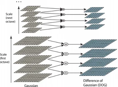
An approximated kernel, called the difference of Gaussian (DoG), is often used in practice instead of using the LoG, since the DoG is more computationally efficient and is a suffi-cient mathematical approximation of the LoG kernel. The DoG approach involves filtering an image with Gaussians of different variances and subtracting them from each other. This operation is effectively a bandpass filter, preserving certain spacial frequencies, determined by the variances used, and results in a blob detector. This DoGD(x,y,σ)is described as

D(x,y,σ) = (G(x,y,kσ)−G(x,y,σ))∗I(x,y) (2.29)

and therefore

=G(x,y,kσ)∗I(x,y)−G(x,yσ)∗I(x,y), (2.30)

since convolution is distributive. Therefore, the subtraction can occur before or after the con-volution process. krepresents a scaling factor that scales one of the Gaussian standard devia-tions with respect to the other in Equadevia-tions 2.29 and 2.30, resulting in a DoG.

(36)

Lowe [44] shows that the relationship between the DoG and scale-normalised LoG can be understood from the appropriated heat diffusion equation described by

σ∇2G= ∂G

∂ σ ≈

G(x,y,kσ)−G(x,y,σ)

kσ−σ , (2.31)

with the partial derivative approximated on the right side. The DoG can then be expressed by

G(x,y,kσ)−G(x,y,σ)≈(k−1)σ2∇2G. (2.32)

The(k−1)factor is constant over all scales and as a result does not influence the locations of the extrema.

Figure 2.9: Visual representation of the scale space, the dimension introduced by blurring the original image, and the construction of the DoG. The image on the left are progressively more blurred from the bottom up. The differences between these images are used to form the DoG. Image reproduced with permission from Lowe [44].

Figure 2.9 illustrates the created scale space and the resultant DoGs. Local extrema need to be searched for in the resulting images by comparing neighbouring pixels across both scale (below and above in scale) and pixel position. This results in a list of potential interest points at a specific scale that might be robust enough for practical use. If interest points are deemed to be robust enough, they will be regarded as features.

The second part consists of locating the interest points (points of interest for feature candidacy) with subpixel accuracy and filtering out interest points that are located on edges. If the subpixel position intensity is less than a certain threshold, then it is also rejected since they would be too sensitive to noise to be robust.

(37)

In order to locate an interest point with subpixel accuracy, a quadratic function is fitted to DoG scale space function. This is achieved by obtaining a second order (quadratic) Taylor series expansion of the scale space functionD, as described by

D(x)≈D(xloc) + ∂DT ∂x x=xloc x+1 2x T ∂2D ∂x2 x=xloc x, (2.33)

with x_loc = [x_loc,y_loc,σ_loc]T denoting the location and scale of the interest point. D(x_loc)

is evaluated at x_loc and denotes the constant Taylor series offset from the linearision point x_loc= (x,y,σ). The three-dimensional quadratic’s local minima or maxima is located where

the gradient of the function is zero, which results in a subpixel point.

The interest points need to be inspected and rejected if the they are located along edges. This filtering process is required because the DoG operation will also yield points along edges as potential feature points. TheHessian matrixHHes, described by

HHes(x,y,σ) = " D_xx D_xy D_xy D_yy # , (2.34)

is used to perform this inspection at the interest point’s location and scale in the scale space function D, with subscripts denoting partial derivatives. Similar to the Harris matrix, the eigenvalues of the matrix are inspected. If both eigenvalues are large, then it indicates large derivatives is all directions, a corner, while only one large (relatively large) eigenvalue indi-cates an edge. Just like the Harris matrix, the ratio of the eigenvalues needs to be smaller than a certain threshold to be regarded as a corner and not an edge. The determinant and trace op-erations can also be used instead of eigenvalue decomposition, like the Harris case described by Equation 2.26, resulting in a more computationally efficient implementation.

Now that points (interest points deemed to be robust) have been identified, with edge re-sponses and noise sensitive points filtered out, these new keypoints need to be described. First an orientation is calculated for each keypoint. This orientation is calculated at each keypoint’s respective scale so that calculations are scale invariant, and will be used to achieve rotation in-variance. In order to calculate the orientation, the gradient magnitudesm(x,y)and orientations

θ(x,y)are computed beforehand for each individual image in the scale spaceL(x,y)(arbitrary

image in the scale space) using the differences of pixel intensities as described by

m(x,y) = r L(x+1,y)−L(x−1,y) 2 + L(x,y+1)−L(x,y−1) 2 (2.35) and

(38)

θ(x,y) =tan−1 L(x,y+1)−L(x,y−1) L(x+1,y)−L(x−1,y) . (2.36)

The calculated gradient orientations in an area around the keypoint are divided into histogram bins. These orientations, depicted on the left side of Figure 2.10, are weighted according to their magnitude, and truncated using a Gaussian window. The largest histogram value/peak indicates the largest local gradient direction. The three closest values to the peak are used as sample points to fit a parabola to the local gradient function. This parabola is then used to interpolate the peak orientation value with increased accuracy, and as a result the keypoint is assigned with an orientation. Before the descriptor is calculated, all of the local gradients are rotated with respect to the determined orientations, resulting in a rotation invariant descriptor.

So far, each keypoint has been assigned a location, scale, and orientation and is done in such a way that the keypoints are invariant to these parameters and to noise. The next step is to assign a descriptor for each keypoint in order to identify the keypoint across multiple images, between stereo images or between images in a time sequence. This descriptor is a function of the local gradients at the keypoint’s position and scale. The left side of Figure 2.10 shows the gradient magnitudes and orientations calculated with the blue circle representing the Gaussian weighting window. The Gaussian window adds more relative weight to the gradients that are closer to the localised position of the keypoint.

Figure 2.10: Visual illustration of a SIFT feature descriptor [4]. The gradient arrows are all added together and weighed in their respective subregion of the image into discrete 45o locations. Image reproduced with permission from Lowe [44].

The divided local gradient orientations are used to determine the descriptor as seen depicted by Figure 2.10. The length of each arrow corresponds to the sum of the gradient magnitudes in their respective directions within each image subregion (section). The directions are discretely

(39)

divided into 8 positions, every 45 degrees, as seen in the figure. The vectors are rotated by the orientation assigned to the keypoint, thereby making the descriptor rotation invariant. As seen in Figure 2.10, 4x4 subregions, comprising, in total, of a 16x16 sample array, are used. The right side of Figure 2.10 visually represents the descriptor of the keypoint. These 4 by 4 subregions with 8 discrete directions results in a 4x4x8 = 128-dimensional vector.

The SIFT feature detector has become a staple in computer vision due to its rotation and scale invariant subpixel features. However, the algorithm is computationally intensive. SURF features were created in order to alleviate some of the computational issues of SIFT.

SURF

SURF (speeded-up robust features) is a computationally more efficient feature detection algo-rithm created by H. Bay et al. in 2006 based on the SIFT algoalgo-rithm. SURF is roughly three times faster than SIFT with slight degradation in accuracy, but still accurate enough to be comparable with SIFT [38]. Considering that the DoG approach, used in the SIFT framework, can be used to approximate the LoG kernel, Bay et al. [21] decided to take the approximation further by approximating the LoG with a box filter, as shown in Figure 2.11. The content is this subsection is reproduced from Bay et al. [21], Guerrero et al. [38], and OpenCV docu-mentation [8].

Figure 2.11: Box kernel approximation (in two dimensions) of the LoGs used in the SIFT framework. The approximation forms the part of basis of the SURF approach [12]. Image reproduced with permission from Tuytelaars [21].

The DoG, which is an approximation of the LoG, is used to create the scale space of image in the SIFT framework. SURF uses a box kernel approximation to create the scale space, which is a further approximation. Initially this approximation would seem computationally more efficient since a LoG does not need to be discretised for every scale, but the real computational advantage is that the convolution process is reduced to simple additions by using an integral image. An integral image is defined by

(40)

II(x,y) = i≤x

∑

i=0 j≤y

∑

j=0 I(i,j). (2.37)

Every point (x,y) in the integral image is equal to the sum of all the pixel intensities in the upper left hand quadrant of the input image. Using a box kernel results in the same operations that are facilitated by the integral image. Figure 2.12 shows how the sum of the pixel inten-sities in a regionΣof the input imageI(x,y)can be computed using the appropriate integral

image II(x,y) values (A, B, C and D) with simple addition and subtraction, approximating the convolution process. Since the integral image does not change with scale, multiple box filtering convolutions can be performed in parallel for different scales, increasing the speed of the algorithm further.

The SURF algorithm uses the Hessian matrix to find interest points in the scale space function after the scale space has been made created using the box filter approximation. The Hessian matrix is described by HHes(x,y,σ) = " L_xx L_xy L_xy L_yy # ≈ " B_xx B_xy B_xy B_yy # (2.38)

with footnotes indicating partial derivatives withL(x,y,σ) =G(x,y,σ)∗I(x,y),Gis a

Gaus-sian kernel. Therefore Lxx is the LoG convolved with the input image. The LoG kernel is approximated with a box filter kernelB(x,y,σ).

Figure 2.12: Illustration of how an integral image is used for box kernel convolution. Image reproduced with permission from Tuytelaars [21].

In order to identify a potential interest point, the determinant of the Hessian is inspected, since eigenvalue decomposition is a computationally expensive operation. The determinant of the Hessian matrix is equal to the product of the eigenvalues, as described by

(41)

|HHes(x,y,σ)|=λ1λ2, (2.39)

and the eigenvalues (λ1,2) give an indication of the gradient deviation of the pixel intensities

which determines if the point is a potential feature. The determinant is calculated using

|HHes(x,y,σ)|=LxxLyy−L2xy≈BxxByy−(0.9Bxy)2. (2.40) The 0.9 factor was empirically determined by Bay et al. [21] to make the box filter kernel approximation more accurate.

SURF uses first order Haar wavelet (Figure 2.13) responses in thexandydirections in order to calculate a keypoint’s orientation and descriptor. The depicted Haar wavelet responses can be calculated using an integral image, which allows for further computational savings since the integral image has already been calculated. The responses give an indication of the local gradients and are weighted with a Gaussian window. The responses are all added in individual subregions of a sliding orientation window of 60o around the keypoint, creating a local dominant gradient vector in each region as the window slides around. Each of these local dominant vectors are compared and the largest is assigned as the keypoint’s orientation as shown in Figure 2.14.

Figure 2.13: First order Haar wavelets. Image reproduced with permission from Tuytelaars [21].

The feature’s descriptor is constructed by creating a vectorv for each subsection around the keypoint. 4x4 subsections are used in total, and the wavelet responses in each subsection are added together to form a four-dimensional vector. These subsections are orientated accord-ing to the dominate keypoint orientation in order to make the resultant descriptor orientation invariant. This four dimensional vector v is made for each of the 4x4 subsections, and is described by v=

∑

dx,

∑

dy,

∑

|dx|,

∑

|dy| . (2.41)

(42)

Figure 2.14: Determining the dominant orientation vector. The red arrow indicates the dom-inant orientation vector for the region under inspection, indicated by grey. The Blue dots represent the individual wavelet responses. Image reproduced with permission from Tuyte-laars [21].

d_x_/_y denotes the wavelet response with respect to the relative dimension, these responses are summed across the 2D pixel position at the scale the keypoint was located. These 4-dimensional vectors for each 4x4 section results in a total 4x4x4 = 64-4-dimensional keypoint descriptor.

SURF also uses the sign of the Laplacian in the feature matching stage. The sign of the Laplacian (positive or negative) indicates if a bright blob is located on a dark background or if a dark blob is located on a bright background. Matching is only considered between features if the two keypoints have the same sign of the Laplacian. The sign of the Laplacian is the trace of the Hessian matrix and therefore has already been calculated and can be used at no extra cost.

SURF offers faster feature detection, but with reduced performance. However, the results are still of such a nature that they are comparable with SIFT. Both SIFT and SURF constructs the scale space using linear diffusion techniques, that is Gaussian based blurring or approxima-tions thereof. A new wave of feature detectors, such as KAZE and A-KAZE, are of interest due to their nonlinear diffusion techniques which results in a unique approach to creating the scale space.

KAZE

In 2012, Alcantarilla et al. [13] proposed a new algorithm for detecting and describing fea-tures called KAZE feafea-tures [13]. KAZE also, like other algorithms, searches for feafea-tures across both scale and pixel position, but constructs the image scale space in a different way.

(43)

Where algorithms like SIFT and SURF construct the scale space with linear diffusion filtering techniques, such as Gaussian blurring, KAZE constructs the scale space by using nonlinear d