Genre-adaptive semantic computing and audio-based modelling for music mood annotation.

Genre-adaptive Semantic Computing and

Audio-based Modelling for Music Mood

Annotation

Pasi Saari, Gy ¨orgy Fazekas,

Member, IEEE,

Tuomas Eerola, Mathieu Barthet,

Member, IEEE,

Olivier Lartillot, and Mark Sandler,

Senior Member, IEEE,

Abstract—This study investigates whether taking genre into account is beneficial for automatic music mood annotation in terms of core affects valence, arousal, and tension, as well as several other mood scales. Novel techniques employing genre-adaptive semantic computing and audio-based modelling are proposed. A technique called the ACTwg employs genre-adaptive semantic computing of mood-related social tags, whereas ACTwg-SLPwg combines semantic computing and audio-based modelling, both in a genre-adaptive manner. The proposed techniques are experimentally evaluated at predicting listener ratings related to a set of 600 popular music tracks spanning multiple genres. The results show that ACTwg outperforms a semantic computing technique that does not exploit genre information, and ACTwg-SLPwg outperforms conventional techniques and other genre-adaptive alternatives. In particular, improvements in the prediction rates are obtained for the valence dimension which is typically the most challenging core affect dimension for audio-based annotation. The specificity of genre categories is not crucial for the performance of ACTwg-SLPwg. The study also presents analytical insights into inferring a concise tag-based genre representation for genre-adaptive music mood analysis. Index Terms—Music information retrieval, mood prediction, social tags, semantic computing, music genre, genre-adaptive.

F

1

INTRODUCTION

M

People tend to use particular genres for mood bal-ancing [1]. Different genres are able to induce distinct emo-tional responses [2] while mood and genre terms are often combined to express musical qualities (e.g. “smooth jazz” and “dark ambient”) [3]. In the field of Music Information Retrieval (MIR), automatic music annotation and retrieval in terms of moods and genres have received considerable attention [4], [5], [6], [7]. Moreover semantic metadata re-lated to mood and genre have been shown to be amongst the most important ones for machine-based semantic music annotation or auto-tagging [8], [9]. It is easy to see why. On one hand, psychological studies have shown that mu-sic can be organised according to perceived and induced (elicited) emotions1 _{[2], [10], and music’s ability to convey} and affect moods is a key factor in explaining why music is culturally important [11]. On the other hand, music genres have traditionally been the most common music content • P. Saari is with the Department of Music, University of Jyvaskyla, 40014

Jyvaskyla, Finland. E-mail: [email protected]

• G. Fazekas, M. Barthet and M. Sandler are with the School of Electronic Engineering and Computer Science, Queen Mary University of London, E1 4NS London, U.K.

E-mail: [email protected]; [email protected]; [email protected]

• T. Eerola is with the Department of Music, Durham University, DH1 3RL Durham, U.K.

E-mail: [email protected]

• O. Lartillot is with the Department for Architecture, Design and Media Technology, Aalborg University, DK-9000 Aalborg, Denmark.

E-mail: [email protected].

Manuscript received Xxxx 00, 0000; revised Xxxxxxx 00, 0000.

1. We employ the words emotion and mood interchangeably in the present paper.

descriptors aiming to categorise music for sales, delivery and consumption (e.g. in retail stores, radio, libraries) [6]. Music genres account for a majority of social tags – free-form textual labels or phrases collaboratively applied to particular resources by users – in online music services such as Last.fm2[12].

Automatic mood annotation or mood prediction of mod-ern online music catalogues that span tens of millions of tracks from numerous genres in a semantically meaningful manner requires advanced computational techniques. Ben-efits of audio-based techniques relying on features related to rhythm, timbre, tonality and others have been shown in numerous music mood annotation studies [4], [13], [14], [15]. In particular, these techniques are beneficial since they solve the cold-start problem [16] of music indexing, providing labels for music not yet rated by people. However, audio-based techniques rely on human-generated ground-truth at the model training stage. Generating such ground-truth for large data sets in a controlled manner is often prohibitively laborious [17]. This may lead to a bottleneck for reaching successful model performance, since the size of the available data may not be sufficiently representative of larger and more heterogeneous music collections.

Other ground-truth sources, more abundant but ar-guably less reliable, have been exploited to deal with the is-sue of limited data availability. These sources can be divided into the games-with-a-purpose [18], [19], online editorial tags [20], [21] and social tags [22], [23]. Of these, social tags provide the most extensive resource for semantic informa-tion on music, but their free-form nature leads to problems related to subjective error and noise, synonymy, polysemy,

and data sparsity [24]. Semantic computing techniques have been employed successfully to tackle these problems [9]. For the purpose of mood annotation, these techniques have been applied in a bottom-up manner to learn emotion models in line with those suggested by research in affective sciences [25], [26]. These learnt models have been deemed efficient as semantic representations [22], [27] and proved robust at smoothing out the noise prevalent in tag data [23]. Audio-based techniques have been applied successfully in conjunction with tag-based semantic computing techniques, either by treating computational audio features as “quasi-tags” alongside textual tags [9], or by mapping the audio features to tag-based semantic layers [20], [28], [29], [30]. The benefit of the latter family of techniques is that they require only the audio file at the prediction stage.

Using large data sources for music mood annotation has two advantages: 1) it enables operating on data that better represent large modern-day music catalogues and thus en-ables tapping into global characteristics of the relationship between music and emotion; and simultaneously, 2) it en-ables drawing information on this relationship at a more detailed level, by considering genre-specific aspects for ex-ample. While audio-based techniques have been efficient at predicting genres [31], mood prediction has remained more elusive [32], especially on the valence dimension, relating to the distinction between positive and negative emotions [14], [30], [33]. Taking into account the genre-specificity of music moods may provide a way to alleviate this issue. Certain mood tags are more relevant to one genre than to another [3] and audio-based mood annotation models trained on sets of tracks drawn from a particular genre give more accurate predictions within the corresponding genres than across genres [34].

Two general approaches have been proposed for audio-based genre-adaptive mood annotation: thegenre-feature ap-proachand thegenre-split/combine approach. The genre-feature approach treats genre tags as conventional input features, either on their own, or alongside a set of audio features [35]. The genre-split/combine approach involves splitting training data into genre subsets, training multiple mood prediction models on these subsets, and when annotating a novel music item, combining the outputs of each model according to the genre of the item. Genre of the novel item may be determined either by pre-specified labels or by using a separate audio-based genre annotation model. In past research, techniques employing the genre-split/combine ap-proach have outperformed equivalent non genre-adaptive techniques [36], [37], whereas techniques employing the genre-feature approach provided a similar level of perfor-mance as techniques employing audio features only [35].

To summarise, employing audio-based techniques, se-mantic computing and genre-adaptivity in music mood annotation have been beneficial in recent studies, while results have been boosted by using semantic computing or genre-adaptivity in conjunction with audio-based tech-niques. However, it has not yet been investigated whether mood prediction performance could be boosted further by genre-adaptive semantic computing or by combining genre-adaptive semantic computing with audio-based techniques. The present study offers the following novel contributions for music mood annotation: 1) it proposes a technique that

employs genre-adaptive semantic computing; 2) it proposes a technique that employs both semantic computing and audio-based mood annotation in a genre-adaptive manner; and 3) it assesses the effect of the specificity of genre cate-gories for genre-adaptive mood annotation. The benefit of the genre-adaptive techniques is evaluated against a num-ber of baseline techniques including non genre-adaptive techniques, conventional auto-tagging and the genre-feature approach. The techniques are trained on a large set of social tag data and audio, and evaluated for the prediction of listeners’ ratings of the perceived moods in a separate set of music tracks.

The rest of the paper is organised as follows: Section 2 discusses how this work relates to the previous studies in MIR. Section 3 describes the data covered in the study while Sections 4 and 5 delineate the techniques to represent and annotate music in terms of mood and genre. Section 6 introduces genre-adaptive mood prediction techniques, and finally, Sections 7 and 8 report the results and conclude the paper.

2

RELATED

WORK

The majority of research in music and mood has utilised either categorical (e.g., happiness, sadness and anger) [26] or dimensional models of emotion. A well-known example of the latter is the affective circumplex [25] which represents different emotions in the underlying dimensions of valence, distinguishing between positive and negative emotions, and arousal, relating to the activity or the intensity aspect of emotion. These dimensions, as well as the tension dimen-sion, spanning from relaxed to tense emotions, have been described as core affects [38], [39]. However, valence and arousal have also been considered as the primary dimen-sions, while tension has been inferred as the product of neg-ative valence and positive arousal [40]. Both the categorical and the dimensional model have been employed in audio-based music mood annotation for classifying music into discrete mood categories [15], [41], [42], or for predicting the core affect and other mood dimensions using regression models [14], [42], [43].

Semantic computing techniques, often based on Latent Semantic Analysis (LSA) [44] have been employed to rep-resent music moods based on tag data. In particular, a model resembling the affective circumplex, inferred in a bottom-up manner from tag data, has been found robust at representing the mood of music [22], [23], [27]. Other representations such as the categorical model have been investigated as well [22]. Saari & Eerola [23] proposed an LSA-based technique called the Affective Circumplex Trans-formation (ACT) that yielded significant improvements over other techniques, as well as raw tags, at predicting listener ratings of the perceived core affects in music. The model training was carried out using social tags from Last.fm and a follow-up study confirmed the results using curated editorial tags associated to production music tracks [21]. The Semantic Layer Projection technique (SLP) was proposed in [29] as an extension to ACT to enhance audio-based music mood prediction. SLP involves projecting tracks to moods via a two-stage process, whereby a corpus of tracks is first mapped based on associated tags to a semantic space

obtained with ACT, and then multiple regression models are trained between audio features and the semantic space. SLP outperformed conventional regression models trained to map audio features directly to listener ratings [29], [30]. ACT and SLP are employed as building blocks of the novel genre-adaptive techniques introduced in the present study.

Several studies have highlighted the challenges of rep-resenting the genre of music. In particular, the finding optimal “resolution” of genres [45] and the fuzziness of genre categories [46] are important problems. In studies attempting to identify the underlying factors of music pref-erences based on genres, four [47] and five [48] underlying factors have typically been singled out. In other studies, 10 [7], 13 [49], and 16 [35] genres have been employed to characterise the typical diversity of music. The analysis of artist tags retrieved from Last.fm highlighted the fuzzi-ness of genre categories [46]: for instance, 56% of artists tagged with “pop” were also tagged with “rock”, and 87% of “alternative” music overlapped with “rock”. Still these three genres have been considered as separate categories in typical music catalogues such as iTunes. The evidence from social tags indicates that a single genre describing a track is not inclusive enough, but perhaps a (weighted) combination of several genre labels would better describe genre information.

Previous approaches to music auto-tagging have gained performance improvements by taking into account the rela-tionships between tags, as observed in their co-occurrence patterns or correlations [50], [51], [52]. For example, Ness et al. [50] trained Support Vector Machine (SVM) models with probabilistic outputs first for multiple tags separately and then used the outputs of each tag-specific model as inputs to second-stage SVMs, which enabled taking into account the relationships between tags. These types of techniques have outperformed non-contextual models and in particu-lar, stacked SVMs have yielded state-of-the-art performance 3_{. However, these techniques exploit tag relationships} irre-spective of whether the tags relate to genres, moods or other concepts.

For audio-based mood annotation, considering genre in particular as contextual information has led to positive results. Lin et al. [37] employed the genre-split/combine approach to the auto-tagging of music in terms of moods, training multiple genre-specific models and combining the models at the annotation stage. They used album-level editorial tags from the Allmusic.com service to represent each music track. Compared to a general model, their genre-adaptive model increased the F-score performance from 0.23 to 0.36. Similar results were obtained in [36] for the classification of music to mood clusters. In comparison with these studies, the present study employes genre-adaptive semantic computing in addition to audio-based modelling and predicts moods represented by dimensions rather than categories or binary classes. Rather than using album-level editorial tags, each track in the test data is rated by several dozens of participants. Moreover, the difference between the nature of the training and test ground-truth, i.e. large-scale but unreliable social tags and reliable listener ratings of 3. cf. http://www.music-ir.org/mirex/wiki/2012:MIREX2012 Results

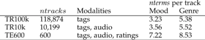
TABLE 1 The employed data sets.

ntermsper track

ntracks Modalities Mood Genre

TR100k 118,874 tags 3.23 5.38

TR10k 10,199 tags, audio 3.56 5.52 TE600 600 tags, audio, ratings 7.22 8.53

mood dimensions, arguably improves the ecological validity of the results thus obtained.

3

DATA

COLLECTION

This section introduces the data comprising mood- and genre-related social tags and associated audio tracks. Table 1 summarises the statistics of the employed data sets, of which TR100k and TR10k are used for model training, and TE600 is reserved for performance evaluation.

3.1 Training Data Sets

The social tag data collected from Last.fm in [23] and reused this study consists of 924k unique tags associated with 1.3M tracks. Each track-tag association is represented by weights in Z[0−100]. As in [23], mood- and genre-related tags were identified by string matching against large lists of mood and genre terms gathered from various sources. For moods, each tag that included a term as a substring was linked to the corresponding term4, whereas for genres, the tags which were kept were only those that fully matched one of the terms. The resulting set was further reduced by keeping only the first 100 mood terms and 100 genre terms that were associated to the highest number of tracks. Tracks performed by artists appearing in TE600, and tracks that were not associated to any mood or any genre term were then excluded.

TR10k, including audio for 10,199 tracks, was sampled from the set resulting from the process above. Full-length CD quality audio files were obtained by accessing the I Like Music (ILM) catalogue, a curated music database with accurate metadata. Last.fm tracks were paired with ILM tracks using controlled track sampling method based on several potentially conflicting criteria. The aim was to ensure a close match between Last.fm and ILM track by using low Levenshtein string distance between the metadata entries (artist, track and album names) with less than 0.5s difference between track durations. The number of tracks within each expert-generated genre category available from ILM was balanced to ensure a fair coverage of different genres overall. The maximum number of tracks sampled from the same artist was limited to avoid artist and album effects. Finally, a three-dimensional mood space obtained by ACT in [23] was used as basis to provide a good coverage of the mood space for each genre. The tracks were sampled such that their distribution in this space is as close to uniform as possible. The resulting TR10k dataset includes tracks from 5,470 unique artists.

4. E.g., tag “happy mood” was thus linked to the term “happy”. If several tags of a track matched the same mood term the highest weight was used.

TR100k was formed by augmenting TR10k with all of the initial corpus that were performed by any artists in TR10k. This was necessary because track sampling excluded important semantic information present in the original set of tracks. This resulted in a set of 118,847 tracks. As seen in Ta-ble 1, the average number of terms associated to each track is higher for genres than for moods, even after the exact string matching of genre terms. This obviously reflects the overall higher prevalence of genre tags than mood tags in social tag data reported in [46]. Within TR10k (and TR100k shown in parentheses), a median of 162 (1,687) tracks are associated to a mood term and a median of 329 (3,869) to a genre term. The most prevalent mood terms are “chillout” (2,569) and “party” (1,638), whereas the least prevalent mood terms are “pleasant” (51) and “bliss” (51). The most prevalent genre terms are “rock” (3,587) and “pop” (3,091), whereas the least prevalent are “root reggae” (147) and “jazz fusion” (150). The relative term prevalences are roughly the same within TR100k.

For the experimental evaluations, 10 training partitions, each comprising 80% of tracks in TR100k or TR10k were ran-domly subsampled from the training data. The subsequent evaluations were thus carried out by performing the model training separately on each training partition and applying the resulting models on the full TE600 set. We will denote the partitions asT (within TR100k) andT0 (within TR10k), T0_⊂T.

3.2 Test Data Set

The TE600 reserved for the evaluation is the same as the one described in [23]. The set consists of 600 tracks with Last.fm tags, audio files and listener ratings of perceived moods. Six broad genres including Metal, Rock, Folk, Jazz, Electronic and Pop are represented in this dataset. The mood ratings were collected from 59 participants on nine step Likert scales for all core affects (Valence, Arousal and Tension) and seven mood terms (Atmospheric, Happy, Dark, Sad, Angry, Sensual, and Sentimental). The ratings were summarised by the average across participants. This deemed sufficient due to the high consistency between the participants reported in [23]). Although listener ratings were obtained for 15 second clips, we use the full tracks in the present study, relying on the claim made in [23] that the clips are representative of the full tracks. The ratings and links to the audio and tag data is publicly available5_.

The tag data associated to TE600 was subjected to a similar process applied to the training sets: each track was linked to the 100 mood and 100 genre terms selected for the training data, and tracks not associated to any mood or genre term were excluded (12 in total).

3.3 Audio Features

62 audio features related to dynamics, onsets, autocorrela-tion, chromagram, and spectrum were extracted from the full-length tracks of TR10k and TE600 using the MIRtool-box6_{[53]. These are summarised in Table 2. The audio} mate-rial was first summed to mono and cut into overlapping

5. http://hdl.handle.net/1902.1/21618 6. MIRtoolbox version 1.5.

TABLE 2

Audio features, aggregated to∗:mm,ms,smandss;†:mmandsm. The “Frame” column reports the window lengths and overlaps (?: 50ms

length with 50% overlap).

Category Feature Stats Frame

Dynamics RMS, Zero-crossing rate

∗ ?

Onsets Attack (time, slope, leap) ∗ Onset-based Event density † 10s, 50% Autocorrelation Pulse clarity, Novelty † 3s, 90%

Tempo † 3s, 33.3%

Chromagram Mode,

HCDF, Key Clarity, Centroid, Novelty

† 750ms, 50%

Spectrum Novelty, Brightness, Centroid, Spread, Flux, Skewness, Entropy, Flatness, Roughness

∗ ?

13 coef. MFCC,∆,∆∆ ∗ ?

analysis frames with feature-specific lengths and degrees of overlap. A frame length of 50ms with 50% overlap was used for low-level spectral features, MFCCs and their first (∆) and second order (∆∆) instantaneous derivatives and for all features related to dynamics. Audio onsets were detected from temporal amplitude curves extracted from a 10-channel filter bank decomposition. Event density was calculated by the number of onsets in 10s, 50% overlapping frames. The features derived from the autocorrelation were calculated using 3s frames with 90% overlap (33.3% overlap for Tempo). Finally chromagrams were computed using 750ms, 50% overlapping frames. From this, several high-level features related to tonality were calculated such as Mode (majorness) and Key clarity.

All features with different frame lengths where brought to the same time granularity by computing the Mean (m) and standard deviation (s) over 1s, 50% overlapping texture windows. However, only the Mean was computed for Event density and in case of the chromagram-related features because they were extracted from longer frames to begin with. Similarly, the standard deviations were omitted for the MFCC derivatives, since their mean values already describe the temporal change. Finally, 178 song-level de-scriptors were obtained by taking again the Mean (mmand ms) and Standard deviation (sm and ss) over the texture window frames. This process is motivated by the approach presented in [50]. Typically the song-level representation of audio features is calculated as the Mean and Standard deviation over the whole track length, excluding the texture window processing. The approach taken here incorporates the temporal dynamics of the features at both short and long time span in a more sensitive fashion compared to the typical song-level averaging approach.

4

GENERAL TECHNIQUES FOR

SEMANTIC

COM-PUTING AND

AUDIO

-BASED

ANNOTATION

Conventional techniques that do not take genre information into account are explained in this section.

4.1 Semantic Computing Using ACT

First, ACT [23] was applied on the training partitions of TR100k to enable representing the mood of tracks based on the associated tags. Initially, associations between mood terms i and tracksj are represented in a standard Vector Space Model (VSM) matrix M = mi,j. As in [23], M

was first normalised by computing Term Frequency-Inverse Document Frequency (TF-IDF) scores and then transformed to a three dimensional semantic mood space by applying non-metric Multi-Dimensional Scaling (MDS). Note, that in [23], dimension reduction was employed in two stages by applying the Singular Value Decomposition (SVD) prior to the MDS. This provided a slight performance improvement compared to dimension reduction with MDS only. However, since the number of mood terms is lower in the present study (100 compared to 357), the SVD stage was excluded. This allowed a reduction in the number of alternative model parameterisations (e.g., the number of dimensions in SVD) in the experiment. In the next stage, a Valence-Arousal space (VA space) was inferred by conforming the semantic mood space to a reference configuration of mood terms (cf. below). This was done using the Procrustes transformation [54] that performs a linear mapping from a space to another while retaining relative distances between objects in the original space. This yields a configurationXi= (xi,1, xi,2, xi,3)of all mood terms in the VA space, retaining the third dimension as in [23].

To apply ACT for mood annotation, a track j repre-sented by mood VSM vector qi,j was projected to the

VA space by first normalizing the vector according to the learned TF-IDF scores yielding qˆ. Then, a representation Sj = (sj,1, sj,2, sj,3) of the track in the VA space was computed by Sj= P iqˆixi P iqˆi . (1)

The final estimates P_j(a) related to the core affects and mood terms were obtained by

P_j(a)= a

|a|·Sj, (2)

whereaequals to the term positions in the configurationXi

for each mood termi, and(1,0,0),(0,1,0), and(−1,1,0)

for Valence, Arousal and Tension respectively.

Of the 101 mood terms present in Russell’s and Scherer’s reference configuration [25], [55], 13 terms could be matched with the 100 mood terms used in the present study. This con-figuration, plotted onto the VA space in Fig. 1a, is denoted byRussell. As one can see, most of the matched terms are located in the low Arousal – high Valence quadrant. Due to this imbalance, a more simple reference configuration was formed by including only one mood term for each VA quadrant: Happy, Calm, Sad, and Angry indicated in boldface in Fig. 1a. This configuration is denotedRussell4. These terms were chosen since they are frequently cited in music and emotion research [56] and their prevalence within TR100k was above the median (10,459,3,554,9,306and1,921 for Happy, Calm, Sad, and Angry respectively).

Affective norm data related to a large set of English lemmas [57] was also explored as a direct alternative to the mood term positions inferred using the ACT. To use this

−1 0 1 −1 0 1 Angry Calm Depressing Happy Hope Joyful Melancholy Passionate Peaceful Pleasant Relaxing Sad Sleepy VALENCE AROUSAL TEN SIO N

(a) Russell (Russell4)

−1 0 1 −1 0 1 Angry Calm Depressing Happy Hope Joyful Melancholy Passionate Peaceful Pleasant Relaxing Sad Sleepy VALENCE AROUSAL TEN SIO N (b) Norms

Fig. 1. Reference mood term configurations from a) Russell [25] and Scherer [55]; and b) Affective norms [57].

configuration, the MDS and Procrustes stages in the ACT were skipped. In addition to Valence and Arousal, the data includes Dominance as the third dimension. 81 mood terms, summarised in Fig. 1b, could be matched between the norm data and tags. This configuration is denotedNorms. To train the model withNorms, 339 tracks had to be excluded from TR10k since they were not associated to any of the matched mood terms.

4.2 Audio-based Annotation Using the SLP

SLP involves training a set of regression models to map audio features to the VA space dimensions learnt using ACT, and applying these models to predict moods in music tracks. In [29] and [30] Partial Least-Squares (PLS) was employed as a regression technique for SLP, whereas in the present study the LIBSVM implementation of Support Vector Regression (SVR) [58] was used. This allowed a direct comparison to an SVM auto-tagger (cf. Section 4.3).

The audio features related to TR10k were z-score-transformed to a zero mean and unit standard deviation. Extreme values were considered outliers and truncated to

[−5,5]. To reduce the SVR training time, highly correlated audio features were removed using agglomerative hierar-chical clustering with the correlation distance function. To this end, the complete linkage criterion with a cutoff cor-relation distance of 0.1 was employed and the first feature in each obtained cluster according to the order presented in Table 2 was kept.

As in Section 4, the VA space was learned using ACT and tracks in the TR10k were projected to the VA space based on the associated tags. SVR models were then trained to map the pre-processed audio feature set to each of the VA space dimensions separately. In a preliminary analysis the SVR was tested using the linear and Radial Basis Function (RBF) kernels, but results indicated that the linear kernel gives a performance comparable to the RBF with a shorter training time. The cost parameterc was set to 0.001 since it yielded consistently high performance compared several candidatesc= 10y_{, y= [−4,−3, ...,1]. SLP was applied on}

the test data to produce audio-based estimatesS_j0. Finally, estimatesP(a)

0

j related to the core affects and mood terms

4.3 Audio-based Annotation using SVM Auto-tagger Two-stage stacked SVMs [50] were employed to compare the SLP performance to a conventional auto-tagger using an implementation following [50]. First, the input audio features of TR10k were pre-processed as described in Sec-tion 4.2 and the mood tags were transformed into binary classes. The first-stage SVM classifiers with a linear kernel and probabilistic outputs were trained separately for each mood and the classifiers were applied on the training tracks. The obtained positive class probabilities for all moods were then served as input to the second-stage SVM classifiers to again map the input to the binary mood classes. When annotating a track in the test data, the models were applied to produce a vector of probability estimates. This vector was normalised to sum to one. Note, that the stacked SVMs are not capable of directly producing estimates for core affects, since Valence, Arousal and Tension are not explicitly represented by any of the mood terms.

Since the mood term prevalence in TR10k varies from 0.5% to 26%, the binary tag data fed to the SVMs is highly imbalanced. In the past, taking into account the class im-balance has yielded positive results for SVM-based music mood auto-tagging [37]. Therefore cost-sensitive learning found effective in [59] was employed by setting differ-ent misclassification error costs for the positive and neg-ative class related to each mood. The costs c+_i = 1 and c−_i =n+_i /n−_i were set for the positive and negative classes respectively (n+_i andn−_i are the number of the positive and negative tracks within the training data for a moodi).

To form another baseline technique, tracks were pro-jected to the VA space based on the outputs of the stacked SVMs. The outputs were TF-IDF-weighted and projected to the VA space as in the ACT prediction stage. This technique, as opposed to the original stacked SVM, is inherently capa-ble of producing estimates also for the core affects. Similar baseline techniques were implemented already in [30] using PLS regression to predict the normalised tag counts, but using stacked SVMs instead proved more efficient as the results will show. These two baseline techniques are denoted SVM-origandSVM-ACT.

5

GENRE

CLUSTERING

REPRESENTATION

BASED ON

TAGS

Prior to exploiting genres as contexts in mood annotation, a sufficiently concise genre representation was sought after. This was done to reduce the computational burden of the mood annotation techniques and because the majority of distinct genres might be too narrow in terms of mood content for within-genre semantic analysis of moods. To this end, genre term clustering was applied to reduce the number of distinct genres.

5.1 Genre Clustering Techniques

Given the associations between genre term i and track j in a VSM matrixG = gi,j, the rows gi were grouped into

disjoint clustersC = {C1, C2, ..., CK} using the following

techniques and specifications:

K-means: G was first normalised to a unit Euclidean

length by ˆ gi,j=gi,j/( X j∈T gi,j2)1/2, (3)

after which the algorithm was run using the cosine distance.

Agglomerative hierarchical clustering: G was first

normalised according to the TF-IDF to produce Gˆ. The cosine distance between gˆi and gˆi0 was then used as the distance measure, and the agglomeration was done based on the average link criterion.

Spectral clustering: G was normalised according

to the TF-IDF, and Cosine similarities between gˆi and ˆgi0 were used as the affinity matrix. Clustering was then done following the method described in [60], similar to [36] where the technique was applied to group emotion tags.

5.2 Genre Clustering Survey and Evaluation

To assess the quality of the obtained genre clusterings, an online genre grouping survey was organised. This also provided insight into the number of genre clusters that would optimally represent the data. The survey task for each participant was to arrange the 100 genre terms into any number of clusters between 2-16 they considered most appropriate. The range for the candidate number of gen-res was selected to acknowledge the typical number of genres assessed in past studies. The instructions specified that the clusters should group genres that share common musical, social or cultural characteristics. The participants were asked to be objective in their assignments, and the instructions allowed using any external web resource to check the definition of possible unfamiliar genre terms (e.g., “downtempo”). 19 participants, predominantly engineering and musicology students knowledgeable of different music genres took part in the survey.

No clear optimal number of genre clusters arose from the survey results. The number of clusters ranged between 6 and 16, with peaks around 9, 10 and 16 clusters (M= 11.34, SD= 3.17). To validate this result, the conventional Davies-Bouldin technique [61] was applied on the genre tag data which allows to infer the optimal number of clusters. This analysis did not yield a clear optimum either. This may re-flect the general difficulty of defining the genre granularity that would satisfy all purposes.

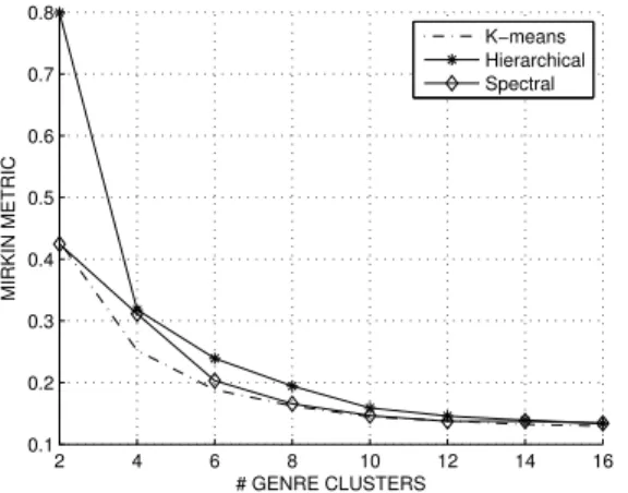
Genre clusterings were computed based on the training partitions of TR100k using K = {2,4,6, ...,16} clusters. The clusterings were compared to those obtained from the survey using the Mirkin metric [62], which can be used to assess the disagreement between two clusterings C={C1, C2, ..., CK}andC‘ ={C‘1, C‘2, ..., C‘K‘}by: dM(C, C‘) = X k n2_k+X k‘ n2_k‘−2X k X k‘ n2_kk‘, (4) wheren andnk are the numbers of genre terms inGand

clusterCk, respectively andnkk‘ is the number of terms in Ck

T

C‘k‘. This metric can be used to compare clusterings with different K. For identical clusterings, dM = 0, and

dM > 0 otherwise. The dM values, computed separately

between the tag-based clusterings and each of the 19 survey clusterings, were averaged across the participants and train-ing partitions. The results are shown in Fig. 2. One can see

2 4 6 8 10 12 14 16 0.1 0.2 0.3 0.4 0.5 0.6 0.7 0.8 # GENRE CLUSTERS MIRKIN METRIC K−means Hierarchical Spectral

Fig. 2. The average Mirkin metric of each genre clustering technique.

TABLE 3

Genre clusters obtained using K-means withK={2,4,6, ...,16}.

K Most prevalent genre term 2 Pop, Rock

4 Soul, Rock, Hard rock, Electronic

6 Hard rock, Singer songwriter, Electronic, Jazz, Rock, Pop 8 Electronic, Rnb, Soul, Instrumental, Pop, Singer songwriter,

Rock, Hard rock

10 Soul, Hip hop, Rock, Electronic, Singer songwriter, Reggae, Alternative, Jazz, Metal, Lounge

12 Electronic, Downtempo, Country, Soul, Hard rock, Punk, Rnb, Singer songwriter, Rock, Jazz, Classic rock, Pop

14 Hip hop, Rock, Singer songwriter, Pop, Pop rock, Jazz, Coun-try, Soul, Metal, New wave, Hard rock, Classic rock, Instru-mental, Electronic

16 Jazz, Rnb, Instrumental, Reggae, Ambient, Pop rock, Rock n roll, Experimental, New wave, Classic rock, Pop, Soul, Electronic, Hard rock, Singer songwriter, Rock

that all clustering techniques compare similarly to the sur-vey data, except that the hierarchical clustering performed poorly withK = 2. In general, K-means outperformed the other techniques by a slight margin. Therefore K-means was used in subsequent analyses.

In order to examine the genre clustering results in more detail, clusterings were computed using K = {2,4, ...,16} based on the full TR100k set. Table 3 shows the most prevalent genre tag for the genre clusters obtained in this manner.

Although the survey did not give clear indication of the optimal number of genre clusters, subsequent analyses were primarily conducted withK = 6. This was the min-imum number obtained in the survey. It also corresponds well with the six broad genre categories of TE600. Fig. 3 shows in detail the discrepancy between the clustering with K = 6and the survey data. For each pair of genre terms the number of participants that assigned both terms to the same cluster was computed. Six genre terms most prevalent in the TR100k are shown for each cluster in the order of prevalence. The six clusters correspond well with the main genres in TE600 since each of these terms are in different clusters. Therefore the clusters are labeled with these genres. One can see from the figure that genre terms in Metal, Folk and Electronic were mostly grouped together also by

Metal Folk Electronic Jazz Rock Pop

19 15 10 4 0 N Hard rock Metal Heavy metal Hardcore Industrial Glam rock Singer songwriter Folk Acoustic Country Folk rock Americana Electronic Dance Electronica Ambient Downtempo Lounge Jazz Instrumental Funk Soundtrack World Smooth jazz Rock Alternative Indie Alternative rock Classic rock Indie rock Pop Soul Rnb Easy listening Hip hop Oldie H ard roc k Metal H ea vy m et al H ardc ore Indus tri al G la m roc k S inge r s ongw ri te r F ol k A cous ti c Count ry F ol k roc k A m eri ca na E le ct roni c D anc e E le ct roni ca A m bi ent D ow nt em po L ounge Jazz Ins trum ent al F unk S oundt ra ck W orl d S m oot h j az z Roc k A lt erna ti ve Indi e A lt erna ti ve roc k Cl as si c roc k Indi e roc k P op S oul Rnb E as y l is te ni ng H ip hop Oldi e

Fig. 3. The discrepancy between the six genre clusters obtained using the K-means, and the cluster co-occurrences of genre terms obtained from the survey.

TABLE 4

The percentage of tracks in the data sets associated to each of the six genre clusters.

Genre cluster TR100k TR10k TE600

Metal 18.2 14.0 27.0 Folk 28.7 34.0 40.3 Electronic 30.3 31.8 46.2 Jazz 33.6 41.3 44.0 Rock 60.1 55.3 80.2 Pop 49.2 57.1 66.2

participants, whereas terms in Jazz, Rock and Pop were not grouped as consistently.

5.3 Track-level Genre Representation

Given the associated genre tags and a genre clustering C, the genre of a track j was represented by a weighted combinationH = hk,j (k∈ {1,2, ..., K}) of the associated

genre clusters: hk,j = P i∈Ckgˆi,j nk X k P i∈Ckˆgi,j nk −1 , (5)

wheregˆi,j was computed with (3) based on the full TR100k

set. Table 4 shows the percentage of tracks in the data sets that are positively associated to each genre cluster. One can see that the clusters are very broad: 80.2% and 66.2% of TE600 tracks belong to Rock and Pop respectively. The high prevalence of tags related to Pop and Rock reflects the fuzziness of these genres.

5.4 Audio-based Genre Annotation using the SVM Auto-tagger

For the audio-based genre annotation stacked SVMs were trained on the genre tags similar to SVM-orig. Given the audio features of a novel track, the vector of genre term probabilities were first predicted, and then the vector was mapped with (5) to the genre clusters obtained using K-means.

6

GENRE-ADAPTIVE

MOOD

ANNOTATION

The adaptive techniques, employing either the genre-feature or the genre-split/combine approach, incorporate ACT for semantic computing and SLP for audio-based an-notation. When the techniques are used to annotate novel tracks, two variants are applied: one predicting genres from tag data and one predicting genres from audio.

It the training phase, these techniques use mood and genre tag data as input: audio featuresA and a clustering of genre termsC ={C1, C2, ..., CK}. The tag-based genre

representation hk,j is then computed with (5). In the

pre-diction phase, tag-based genre representation is computed again with (5), whereas audio-based genre representation is computed as described in Section 5.4.

6.1 Genre-feature Techniques

The genre-feature techniques use genre information as nor-mal input features for SLP training:

Genre-based Prediction (SLPg): SLPginvolves

pre-dicting mood using only the genre information as input giving an indication as to how much variance of mood ratings can be attributed to mood prevalence differences between genres. SLPgdiffers from the general SLP in that the input features are represented byhk,j instead of audio

features – all other stages are the same as in general SLP.

Genre- and Audio-based Prediction (SLPga): SLPga

is similar to SLPg, but uses the audio features alongside the genre information. The data is therefore represented by

(h1,j, h2,j, ..., hK,j, a1,j, a2,j, ..., an,j), wheren is the

num-ber of features after pre-processing. 6.2 Genre-Split/Combine Techniques

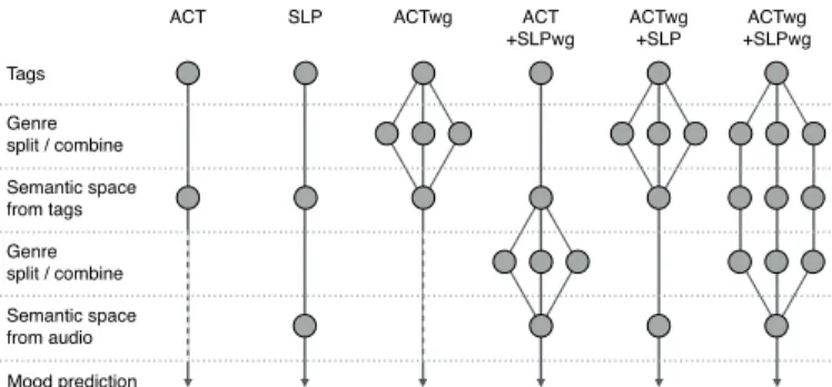
All genre-split/combine techniques involve splitting train-ing data into (possibly overlapptrain-ing) genre subsets, for either ACT training (denoted by ACTwg), SLP training (denoted by SLPwg), or both (denoted by ACTwg-SLPwg). The ACT training is performed within TR100k, whereas SLP training is performed within TR10k. Splitting is done based on the genre tags so that a subset related to genrekcomprises the tracks{j:hk,j>0}. Fig. 4 shows how the techniques differ

from the general form of ACT and SLP.

Genre-adaptive Semantic Computing (ACTwg):

ACTwg is based on the assumptions that relationships of moods vary between genres and that genre-specific seman-tic models are required to boost the mood annotation perfor-mance of semantic computing. The final model combining these genre-specific models would then sufficiently account for the variation between genres. To train the ACTwg model, Kmood term configurationsXikin genre-specific VA spaces

are learned using ACT and at the prediction stage, these Tags Genre split / combine Semantic space from tags Genre split / combine Semantic space from audio

ACT SLP ACTwg ACT +SLPwg ACTwg +SLP ACTwg +SLPwg Mood prediction

Fig. 4. A schematic diagram showing the different stages at which genre-adaptivity is applied in the genre-split/combine techniques.

models are applied to produce the genre-specific estimates P(ak)k

j . The final estimates are then computed by weighting

the genre-specific estimates proportionately tohk:

P_j(a)=P 1 khk,j X k hk,jP (ak)k j . (6)

Audio-based modelling within Genres

(ACT-SLPwg): In ACT-SLPwg, the general type of semantic

com-puting is performed and only the audio-based SLP models are trained within each genre subset. The assumption un-derlying this technique is that audio features and feature combinations relate to moods differently within different genres. SLP models are trained on each genre subset as described in Section 4.2. Applying these models on novel tracks produces genre-specific estimates P(a)

0 k

j . The final

estimates are then computed similar to (6): P(a) 0 j = 1 P khk,j X k hk,jP (a)0_k j . (7)

Genre-adaptive Semantic computing and

audio-based modelling (ACTwg-SLP): In ACTwg-SLP, it is

as-sumed that genre-adaptive semantic computing is needed but that the relationship between audio and VA space dimensions remains static across genres. First, genre-specific ACT models are trained similarly to ACTwg, and the models are applied on the tracks in the training data to produce the estimates for the mood dimensions:

Sj= 1 P khk,j X k hk,jSjk. (8)

Then, general SLP models are trained to map the audio to Sj. At the prediction stage, the general SLP models

are applied to produce P(ak)0

j and the final estimates are

computed by P_j(a)0 =P 1 khk,j X k hk,jP (ak)0 j . (9)

adaptive Semantic Computing and

Genre-adaptive Audio-based modelling (ACTwg-SLPwg):

ACTwg-SLPwg employs genre-adaptivity in both semantic computing and audio-based modelling, assuming that both the semantic relationships of mood terms and audio-to-mood associations vary between genres. First, genre-specific ACT models are trained on each genre subset and the models are applied on the training data to produce Sk

Then, genre-specific SLP models are trained to map audio to Sjk. At the prediction stage, the final estimates are computed

by P(a) 0 j = 1 P khk,j X k hk,jP (ak)0k j . (10)

7

RESULTS AND

DISCUSSION

The annotation performance of the techniques was evalu-ated in terms of the coefficient of determination statistic (R2

) after fitting simple linear regression models between the estimates and the listener ratings. TheR2-statistic was chosen as the goodness-of-fit measure since it is used in the bulk of past studies on automatic prediction of Arousal and Valence for music7. Median and median absolute deviation (MAD) across the models trained on each of the training partitions of TR100k and TR10k are reported.

7.1 General Techniques

7.1.1 Tag-based Annotation

First, the performance of the ACT models trained using the different mood term configurations was compared so as to choose the most successful configuration for subsequent analyses. The results are shown in Table 5. In general, the core affects were more easy to predict than the mood terms, and the performance for Valence was lower than for Arousal. These findings are in line with those obtained from past work evaluating ACT with TE600 data [23], [30]. Russell4 yielded the highest performance for seven mood scales, and was clearly more efficient thanRussellfor Dark and Sad. These mood terms were also among the most difficult to predict. On the other hand, Russell was more successful at predicting Valence, Tension and Atmospheric. Norms yielded dramatically lower performance than the other configurations, which arguably supports exploiting music-specific data to form the semantic mood space, rather than using a mood configuration that relates to affective connotations of mood words in general. It also indicates that the inclusion of Dominance as the explicit third dimension in the mood space does not provide clear benefits. When examining the average performance across mood scales, Russell4 (R2 _{= 0.387) outperformed Russell by a slight} margin (R2 _{= 0.371}

). This suggests that ACT is not overly sensitive to changes in the mood reference configuration and that a simple reference configuration provides a strong enough reference to reliably represent mood terms in the VA space. Therefore,Russell4was chosen for the subsequent audio-based analyses.

The VA space obtained using Russell4 is presented in Fig. 5. The mood positions for the figure were computed as the average of those obtained from each training partition. The underlying dimensions of Valence and Arousal are easily distinguishable, and the obtained positions for the four reference terms correspond fairly well with the original positions, with the exception of Sad, which is close to neutral in the Valence dimension. This finding is in line with [10], where musical examples expressing sadness were perceived as neutral in terms of Valence.

7. This statistic equals to the squared Pearson’s correlations and was chosen since the mood estimates, roughly within[−1.5,1.5], are scaled differently to the ratings, which were given on scales from 1 to 9.

TABLE 5

Prediction results for ACT withRussellandRussell4reference configurations andNorms.

Russell Russell4 Norms Valence 0.4250.013 0.4130.015 0.2700.000 Arousal 0.4770.004 0.4860.003 0.2690.000 Tension 0.3820.015 0.3780.014 0.2190.001 Atmospheric 0.4240.039 0.3950.026 0.1570.000 Happy 0.3840.016 0.3860.011 0.3000.000 Dark 0.2740.087 0.3480.035 0.0380.000 Sad 0.2010.015 0.2760.013 0.1660.000 Angry 0.5220.013 0.5310.017 0.2140.000 Sensual 0.4030.006 0.4160.007 0.0020.000 Sentimental 0.2200.020 0.2380.023 0.0610.000 Average 0.371 0.387 0.170 −1.5 −1 −0.5 0 0.5 1 1.5 −1.5 −1 −0.5 0 0.5 1 1.5 Light Laidback Good mood Exuberant Uptempo Cheerful Pleasant Positive Optimistic Lazy Playful Jazzy Smooth Joyful Warm Religious Dramatic Depressing Heavy Intense Dark Epic Melodic Sad Emotional Moody Progressive Melancholy Eclectic Inspiring Bittersweet Atmospheric Erotic Wistful Intelligent Sardonic Passionate Dreamy Psychedelic Reflective Chillout Nostalgia Romantic Hope Happy Sexy Slow Relaxing Mellow Trippy Uplifting Sentimental Sensual Summer Sweet Dancing Deep Soft Soulful Funky I feel good Easy Groovy Sleepy Gentle Silly Bouncy Peaceful Upbeat Bliss Quiet Soothing Party Calm Meditation Fun Rockin Quirky Ethereal Fast Spiritual Humor Haunting Cynical Sarcastic VALENCE Hypnotic Energetic Loud Power Lyrical Sleazy Make me cry Guilty pleasure Spooky Angry Aggressive Horror Brutal Technical Black AROUSAL TEN SIO N

Fig. 5. Mood tag positions (the averages across training partitions) obtained with ACT usingRussell4as the reference configuration.

7.1.2 Audio-based Annotation

Table 6 presents the performance obtained with SLP (us-ingRussell4) and stacked SVMs. The audio-based mapping onto the VA-space using SLP provided dramatically higher performance than the tag-based mapping using ACT for all mood scales except for Valence, Happy, and Dark – all of which in fact relate to either positive or negative moods. The clearest difference between the SLP and the ACT was obtained for Arousal (R2 _{= 0.728 vs. 0.477). This rather} surprising result, although congruent with that reported in [30], may be explained by the sparsity and the inherent unreliability of tag data: the ACT maps tracks to the mood space based on only few tags, which may cause local incon-sistencies. By contrast, mapping audio features to the mood dimensions using SLP may tap into more global patterns and provide a way to “smooth out” these inconsistencies. The mean SLP performance across mood scales was similar to that reported in [30] (R2 _{= 0.455 vs.0.453). However,} prediction performance for Valence was clearly higher in the present study,R2= 0.359compared toR2= 0.322.

TABLE 6

Prediction results for SLP and SVM baseline techniques.

SLP SVM-orig SVM-ACT Valence 0.3590.019 – 0.3690.020 Arousal 0.7280.004 – 0.7140.005 Tension 0.4850.019 – 0.4830.022 Atmospheric 0.6960.014 0.0690.004 0.6840.020 Happy 0.3120.030 0.2050.003 0.3140.031 Dark 0.2350.023 0.3110.004 0.2480.020 Sad 0.3030.011 0.3160.007 0.3230.007 Angry 0.5890.016 0.6220.008 0.6180.017 Sensual 0.5440.004 0.2520.026 0.5350.010 Sentimental 0.3000.024 0.4360.016 0.3040.030 Average 0.455 0.316 0.459 TABLE 7

Genre prediction performance in terms of median and MAD across training partitions.

Precision Recall AP AROC Metal 0.7760.010 0.5690.003 0.8260.004 0.8410.002 Folk 0.6420.010 0.5310.015 0.7340.006 0.7550.003 Electronic 0.8000.010 0.5150.009 0.8520.005 0.7690.002 Jazz 0.6980.013 0.5770.004 0.7950.006 0.7660.003 Rock 0.9180.004 0.5240.003 0.9390.001 0.7310.001 Pop 0.8500.004 0.6290.011 0.8880.004 0.7810.003

(employingRussell4) increased the performance by a clear margin. Low performance of SVM-orig for Atmospheric, Happy, and Sensual suggests that the way these tags are applied by Last.fm users is not accounted well by musical characteristics, and that the musical characteristics congru-ent with these mood dimensions are better modelled by more general patterns incorporated in a low-dimensional mood space. Although SVM-ACT provided performance comparable to SLP, the benefit of SLP is lower computation-ally complexity requiring one audio-based model for each VA space dimension. Therefore, SLP may be considered the best-performing technique to be used as the baseline for genre-adaptive techniques.

7.2 Audio-based Genre Prediction

Performance of audio-based genre prediction was assessed by comparing the predicted values to the tag data. Al-though the reliability of social tags is questionable, the tag-based evaluation was considered sufficient for the present study because of the subsidiary role of audio-based genre prediction. Table 7 shows the performance for each genre cluster in terms of the standard evaluation metrics Preci-sion, Recall, Average Precision (AP) and the area under the ROC curve (AROC). For each track, the SVM produces probability estimates related to the association strength of each genre cluster. To compute the Precision, Recall and AP, three genres with the highest probability were considered as positive for each track. AROC, on the other hand, was com-puted based on all probability values8_{. The results showed} that genre prediction from audio is sufficient (see [8] for comparison) and may be used as an alternative to tag-based genre inference.

8. See [8] for detailed explanation of these metrics

TABLE 8

Performance of the genre-feature techniques with genres inferred from tags and audio. Performance improvements over the SLP are

highlighted.

Tag-based genres Audio-based genres

SLPg SLPga SLPg SLPga Valence 0.3720.003† 0.4530.008∗ 0.3460.003† 0.4000.020† ∗ Arousal 0.1460.004† ∗ 0.7020.004† ∗ 0.2340.004† ∗ 0.7310.005 Tension 0.2780.007† ∗ 0.4630.012† ∗ 0.3490.009† ∗ 0.4940.018† Atmosph. 0.2050.016† ∗ 0.6620.025∗ 0.2940.013† ∗ 0.7040.021 Happy 0.2210.003† ∗ 0.3980.020∗ 0.1750.002† ∗ 0.3320.034† Dark 0.3790.011† ∗ 0.3780.025† ∗ 0.3260.016† ∗ 0.2710.019 Sad 0.0000.000† ∗ 0.2710.023† ∗ 0.0090.002† ∗ 0.2960.009† Angry 0.5010.004† ∗ 0.6470.009∗ 0.5710.008† ∗ 0.6300.019∗ Sensual 0.3410.015† ∗ 0.5320.026 0.3790.008† ∗ 0.5460.009 Sentim. 0.0580.003† ∗ 0.2460.021† ∗ 0.0960.003† ∗ 0.2960.028† Average 0.250 0.475 0.278 0.470

†_{p < .05for performance difference between the ACTwg-SLPwg.} ∗_{p < .05for performance difference between the SLP.}

7.3 Genre-adaptive Techniques

To assess the statistical significance of performance differ-ences between the general and the genre-adaptive tech-niques, Wilcoxon rank sum tests were carried out across models trained on the training partitions. The techniques involving audio-based mood prediction were compared to general SLP (see Table 6), whereas ACTwg was compared to the general ACT (seeRussell4 in Table 5). Furthermore, equivalent comparisons were carried out between each tech-nique and ACTwg-SLPwg. Results for the genre-feature and the genre-split/combine techniques are presented in Tables 8 and 9, respectively.

7.3.1 Genre-feature Approach

Among the techniques employing the genre-feature ap-proach, SLPga performed well compared to general SLP. With audio-based genres, it outperformed the general model for all mood scales except for Sad and Sentimental. It yielded clear improvements of the average performance across mood scales. On the other hand, already the SLPg, relying only on genres as inputs, yielded relatively high performance for Valence, the most challenging core affect for general SLP. Moreover, with the genre-split/combine tech-niques included, SLPg was interestingly the most successful technique for Dark, which indicates that Dark correlates highly with genre information.

7.3.2 Genre-split/combine Approach

Results for ACTwg showed that genre-adaptive semantic computing is beneficial for tag-based mood annotation. ACTwg outperformed general ACT for all mood scales except for Atmospheric and Sensual. This performance dif-ference was significant for five scales. Performance improve-ment over the ACT was the most notable for Valence with ACTwg reachingR2_{= 0.457.}

Genre adaptivity of audio-based modelling using ACT-SLPwg improved the performance especially for Valence, Happy, Dark, and Angry, which suggests that the musical characteristics correlating with moods related to the pos-itive/negative emotions differ between genres. With the exception of Angry, these mood scales were also among

the most difficult to predict using the general SLP. ACTwg-SLP also improved the performance over general ACTwg-SLP and yielded performance comparable to that of ACT-SLPwg. In general however, these techniques were not significantly more effective than the more simple genre-feature technique SLPga.

ACTwg-SLPwg yielded the highest performance. The average performance across moods was R2 _{= 0.482 with} tag-based genres and R2 = 0.492 with audio-based gen-res. These figures are considerably higher than that of the general SLP (R2 _{= 0.455). Notably, ACTwg-SLPwg with} audio-based genres gave statistically significant improve-ments over SLP for seven mood scales and importantly for all core affects. The clearest performance improvement was achieved for Valence, where the ACTwg-SLPwg yielded R2 = 0.457 with tag-based genres andR2 = 0.431 with audio-based genres. Also for Arousal and Tension, ACTwg-SLPwg with audio-based genres yielded the highest per-formance of R2 = 0.741,0.520 respectively. The fact that audio-based genre prediction for mood annotation performs comparably to tag-based genres indicates that relying solely on audio in making predictions for novel tracks is a viable approach when human-generated semantic data are not available.

To further confirm the benefit of genre-adaptivity, ACTwg-SLPwg was applied to TE600 by first randomly rearranging the tag- and audio-based genre weights. It was assumed that if the high performance of ACTwg-SLPwg thus obtained would not degrade, the performance could be attributed to the benefit of ensemble modelling [63] and not to genre-adaptivity. The analysis showed that this is not the case. The genre randomisation degraded the prediction performance consistently. The average performance across mood scales dropped to R2 _{= 0.424,0.400 using tag- and} audio-based genres respectively, and the performance differ-ence was statistically significant atp <0.05for seven scales (tag-based genres) and for all scales (audio-based genres).

In summary, the results suggest that genre-adaptivity in both audio-based modelling and semantic computing is beneficial and that combining these two forms of genre adaptivity yields the highest performance improvements for music mood annotation.

7.3.3 Comparison of ACTwg-SLPwg and Genre-specific Models

If automatic music annotation is applied to a music col-lection representing one particular genre, one could ask whether a genre-specific model corresponding to the match-ing genre would be more appropriate than ACTwg-SLPwg. Such hypothesis was tested by comparing the prediction performance of ACTwg-SLPwg for the core affects sep-arately on subsets of TE600 associated to the six genre clusters. TE600 was split for this purpose using tag-based genres. Table 10 showsthe results obtained with SLP for each subset. The genre-spcific ACTwg-SLPwg sub-model corresponding to the genre of the subset (using no genre-weighting, see (10)), and ACTwg-SLPwg with audio-based genres.

In this analysis, ACTwg-SLPwg yielded consistently higher performance than the genre-specific models and SLP, with only few exceptions: Valence/Electronic,

TABLE 10

Prediction performance of SLP, genre-specific model and ACTwg-SLPwg separately for tracks from different genres.

SLP Genre- ACTwg specific -SLPwg Valence Metal 0.3870.020 0.4070.011 0.421∗0.008 Folk 0.1990.019 0.1270.037 0.267∗0.006 Electronic 0.2390.022 0.339∗0.009 0.316∗0.014 Jazz 0.2670.024 0.3050.021 0.360∗0.012 Rock 0.3110.019 0.351∗0.003 0.378∗0.004 Pop 0.2250.020 0.299∗0.009 0.306∗0.006 Arousal Metal 0.7200.006 0.5840.011 0.7130.008 Folk 0.7030.006 0.6740.006 0.715∗0.003 Electronic 0.7350.004 0.7270.003 0.748∗0.003 Jazz 0.6710.009 0.6420.008 0.6860.008 Rock 0.7230.005 0.7070.006 0.733∗0.006 Pop 0.7130.004 0.7160.002 0.723∗0.004 Tension Metal 0.5410.014 0.4990.022 0.5710.004 Folk 0.3790.022 0.3210.030 0.415∗0.007 Electronic 0.3720.019 0.424∗0.030 0.415∗0.007 Jazz 0.3580.020 0.3360.011 0.399∗0.007 Rock 0.4730.018 0.4690.005 0.505∗0.004 Pop 0.4260.025 0.4430.009 0.465∗0.010 ∗_{p < .05for improvement over SLP.}

Arousal/Metal and Tension/Electronic. Compared to gen-eral SLP, the genre-specific models were more successful at predicting Valence, which provides further evidence that genre-specific aspects need to be taken into account when modelling the Valence dimension. On the other hand, the re-sults for Arousal showed an opposite pattern. These rere-sults corroborate the findings of [34], where audio-based genre-specific models of Arousal generalised better across genres than those of Valence.

Overall, the genre-adaptive technique was clearly more successful than the specific models. Since genre-specific models rely on training data from one genre, the models may suffer from low variance in the mood content, and might not therefore tap into more general relationships between audio features and mood, only attainable from collections of tracks spanning multiple genres.

7.3.4 The Impact of the Number of Genres

To explore the role of the number of genre clusters on the performance of ACTwg-SLPwg with audio-based genres, analysis was carried out using the genre clusterings with 2-16 genres (cf. Table 3). The results shown in Fig. 6, demonstrates that ACTwg-SLPwg performance is not overly sensitive to the number of genres. Performance consistently remains at a higher level than that of SLP on all genre clusterings. The optimal performance was found for all of the core affects atK= 6, which may possibly be attributed to the fact that TE600 is balanced according to the corre-sponding genres.

8

CONCLUSION

The present study examined how genre information can be incorporated into music mood prediction using genre-adaptive semantic computing and genre-genre-adaptive audio-based modelling. As the general baseline technique, SLP performed favourably when compared to a state-of-the-art auto-tagging method. The comparison with genre-adaptive

TABLE 9

Performance of the genre-split/combine techniques with genres inferred from tags and audio. Performance improvements over the ACT (ACTwg) or SLP (other techniques) are highlighted.

Tag-based genres Audio-based genres

ACTwg ACT ACTwg ACTwg ACTwg ACT ACTwg ACTwg

-SLPwg -SLP -SLPwg -SLPwg -SLP -SLPwg Valence 0.4570.005∗ 0.4340.017† ∗ 0.4060.004† ∗ 0.4570.004∗ 0.4560.004† ∗ 0.3970.018† ∗ 0.4060.004† ∗ 0.4310.004∗ Arousal 0.4880.003† 0.7220.006 0.7410.002† ∗ 0.7320.003 0.4890.004† 0.7250.006† 0.7410.002∗ 0.7410.005∗ Tension 0.3970.004† ∗ 0.5050.017 0.5130.005† ∗ 0.5180.004∗ 0.4000.005† ∗ 0.4970.017† 0.5130.005∗ 0.5200.005∗ Atmospheric 0.3910.033† 0.6890.013† 0.7000.011† 0.6310.035∗ 0.4230.027† 0.6990.014 0.7030.012 0.6890.024 Happy 0.4310.004† ∗ 0.3670.032∗ 0.3580.014† ∗ 0.3890.006∗ 0.4340.008† ∗ 0.3310.031† 0.3620.017∗ 0.3690.012∗ Dark 0.3660.027† 0.3000.025∗ 0.1970.026† ∗ 0.2680.041 0.3810.025† 0.2750.021 0.2080.031∗ 0.2700.037 Sad 0.3100.005† ∗ 0.2880.012† 0.3330.008∗ 0.3300.005∗ 0.3170.007† ∗ 0.2910.011† 0.3400.007∗ 0.3380.006∗ Angry 0.5530.005† ∗ 0.6430.016∗ 0.6030.008† ∗ 0.6430.006∗ 0.5520.007† ∗ 0.6290.017∗ 0.6020.007† 0.6390.004∗ Sensual 0.3570.024† ∗ 0.5460.009† 0.4800.047∗ 0.5170.045 0.3840.015† 0.5450.011 0.5110.024† ∗ 0.5460.021 Sentimental 0.2550.008† 0.2820.027 0.3340.015 0.3380.017 0.2830.013† ∗ 0.2890.026† 0.3690.019 0.3770.017∗ Average 0.401 0.478 0.466 0.482 0.412 0.468 0.476 0.492

†_{p < .05for performance difference between the ACTwg-SLPwg.}

∗_{p < .05for performance difference between the ACT (ACTwg) or the SLP (other techniques).}

SLP 2 4 6 8 10 12 14 16 0.35 0.4 0.45 0.5 0.55 0.6 0.65 0.7 0.75 R 2 Valence Arousal Tension

Fig. 6. The Median±MAD performance of ACTwg-SLPwg using genre clusterings with 2-16 genres. The SLP performance is shown for com-parison.

models showed that taking into account the genre in-formation in mood annotation yields consistent improve-ments. The highest performing novel technique ACTwg-SLPwg models both the semantic mood space and audio-to-mood relationship in a genre-adaptive manner. Moreover, audio-based genre inference for a novel track performed favourably compared to tag-based inference, which has positive implications for applying the models to large unan-notated datasets.

The study also offered survey results and analytical insights into inferring concise music genre representations based on a large set of genre tags. Moreover, the study demonstrated that semantic modelling of mood space based on music-specific social tag data is not surpassed by non-music-specific normative data obtained from a controlled laboratory survey.

The proposed techniques could be applied to other tasks, such as object recognition from images, video auto-tagging, or multimedia retrieval, where context-adaptive semantic

modelling combined with context-adaptive content-based prediction could be beneficial.

ACKNOWLEDGMENTS

The work of Pasi Saari is funded by the Academy of Finland (The Finnish Centre of Excellence in Interdisciplinary Music Research). The work of Gy ¨orgy Fazekas and Mark Sandler is funded by the EPSRC programme grant “Fusing Semantic and Audio Technologies for Intelligent Music Production and Consumption” (FAST-IMPACt) EP/L019981/1.

REFERENCES

[1] T. Sch¨afer and P. Sedlmeier, “From the functions of music to music preference,”Psychology of Music, vol. 37, no. 3, pp. 279–300, 2009. [2] M. R. Zentner, D. Grandjean, and K. Scherer, “Emotions evoked

by the sound of music: Characterization, classification, and mea-surement,”Emotion, vol. 8, no. 4, pp. 494–521, 2008.

[3] X. Hu and J. S. Downie, “Exploring mood metadata: relationships with genre, artist and usage metadata,” inProceedings of the 8th In-ternational Conference on Music Information Retrieval (ISMIR), 2007. [4] M. Barthet, G. Fazekas, and M. Sandler, “Multidisciplinary

per-spectives on music emotion recognition: Recommendations for content- and context-based models,” in Proceedings of the 9th International Symposium on Computer Music Modeling and Retrieval (CMMR), 2012, pp. 492–507.

[5] Y. E. Kim, E. M. Schmidt, R. Migneco, B. G. Morton, P. Richardson, J. Scott, J. A. Speck, and D. Turnbull, “Music emotion recognition: A state of the art review,” inProceedings of the 11th International Conference of Music Information Retrieval (ISMIR). Citeseer, 2010, pp. 255–266.

[6] N. Scaringella, G. Zoia, and D. Mlynek, “Automatic genre classifi-cation of music content,”IEEE Signal Processing Magazine : Special Issue on Semantic Retrieval of Multimedia, vol. 23, pp. 133–141, 2006. [7] G. Tzanetakis and P. Cook, “Musical genre classification of audio signals,”IEEE Transactions on Speech and Audio Processing, vol. 10, no. 5, pp. 293–302, 2002.

[8] D. Turnbull, L. Barrington, D. Torres, and G. Lanckriet, “Semantic annotation and retrieval of music and sound effects,”IEEE Trans-actions on Audio, Speech, and Language Processing, vol. 16, no. 2, pp. 467–476, 2008.

[9] M. Levy and M. Sandler, “Music information retrieval using social tags and audio,”IEEE Transactions on Multimedia, vol. 11, no. 3, pp. 383–395, 2009.

[10] T. Eerola and J. Vuoskoski, “A comparison of the discrete and dimensional models of emotion in music.” Psychology of Music, vol. 39, no. 1, pp. 18–49, 2011.