College of Engineering, Mathematics and Physical Sciences
Statistical methods for
post-processing ensemble weather
forecasts
Robin Mark Williams
Supervised by Dr Christopher A. T. Ferro & Dr Frank
Kwasniok
Submitted by Robin Mark Williams, to the University of Exeter as a thesis for the degree of Doctor of Philosophy in Mathematics , February 2016.
This thesis is available for Library use on the understanding that it is copy-right material and that no quotation from the thesis may be published without proper acknowledgement.
I certify that all material in this thesis which is not my own work has been identified and that no material has previously been submitted and approved for the award of a degree by this or any other University.
Until recent times, weather forecasts were deterministic in nature. For example, a forecast might state “The temperature tomorrow will be 20◦C.” More recently, however, increasing interest has been paid to the uncertainty associated with such predictions. By quantifying the uncertainty of a forecast, for example with a proba-bility distribution, users can make risk-based decisions. The uncertainty in weather forecasts is typically based upon ‘ensemble forecasts’. Rather than issuing a sin-gle forecast from a numerical weather prediction (NWP) model, ensemble forecasts comprise multiple model runs that differ in either the model physics or initial con-ditions. Ideally, ensemble forecasts would provide a representative sample of the possible outcomes of the verifying observations. However, due to model biases and inadequate specification of initial conditions, ensemble forecasts are often biased and underdispersed. As a result, estimates of the most likely values of the verifying obser-vations, and the associated forecast uncertainty, are often inaccurate. It is therefore necessary to correct, or post-process ensemble forecasts, using statistical models known as ‘ensemble post-processing methods’. To this end, this thesis is concerned with the application of statistical methodology in the field of probabilistic weather forecasting, and in particular ensemble post-processing. Using various datasets, we extend existing work and propose the novel use of statistical methodology to tackle several aspects of ensemble post-processing.
Our novel contributions to the field are the following. In chapter 3 we present a comparison study for several post-processing methods, with a focus on probabilistic forecasts for extreme events. We find that the benefits of ensemble post-processing are larger for forecasts of extreme events, compared with forecasts of common events. We show that allowing flexible corrections to the biases in ensemble location is im-portant for the forecasting of extreme events. In chapter 4 we tackle the compli-cated problem of post-processing ensemble forecasts without making distributional assumptions, to produce recalibrated ensemble forecasts without the intermediate step of specifying a probability forecast distribution. We propose a latent variable model, and make a novel application of measurement error models. We show in three case studies that our distribution-free method is competitive with a popular alter-native that makes distributional assumptions. We suggest that our distribution-free method could serve as a useful baseline on which forecasters should seek to
im-subject to uncertainty. We approximate the distribution of model parameters by bootstrap resampling, and demonstrate improvements in forecast skill by incorpo-rating this additional source of uncertainty in to out-of-sample probability forecasts. In chapter 6 we use model diagnostic tools to determine how specific post-processing models may be improved. We subsequently introduce bias correction schemes that move beyond the standard linear schemes employed in the literature and in practice, particularly in the case of correcting ensemble underdispersion. Finally, we illustrate the complicated problem of assessing the skill of ensemble forecasts whose members are dependent, or correlated. We show that dependent ensemble members can result in surprising conclusions when employing standard measures of forecast skill.
List of tables 8
List of figures 10
1 Introduction 13
2 Ensemble weather forecasting and ensemble post-processing 17
2.1 Introduction . . . 17
2.2 Numerical weather prediction and ensemble weather forecasting . . . 17
2.2.1 Introduction . . . 17
2.2.2 Numerical weather prediction . . . 18
2.2.3 From deterministic forecasts to ensemble forecasts . . . 20
2.2.4 Interpretations of ensemble forecasts . . . 23
2.3 Forecast calibration and forecast uncertainty . . . 25
2.3.1 Calibration for probability forecasts . . . 25
2.3.2 Calibration for ensemble forecasts . . . 26
2.4 An overview of ensemble post-processing methods . . . 27
2.4.1 Introduction . . . 27
2.4.2 Ad-hoc post-processing methods . . . 30
2.4.2.1 Frequency-based probability forecasts . . . 30
2.4.2.2 Rank histogram recalibration . . . 31
2.4.3 Ensemble dressing methods . . . 33
2.4.3.1 Best member dressing . . . 33
2.4.3.2 Bayesian model averaging . . . 35
2.4.4 Regression methods . . . 37
2.4.4.1 Model output statistics . . . 37
2.4.4.2 Nonhomogeneous Gaussian Regression . . . 37
2.4.4.3 Logistic regression . . . 40
2.4.5 Miscellaneous post-processing methods . . . 42
2.4.6 Ensemble copula coupling . . . 44
2.4.7 Parameter estimation . . . 47
2.4.7.1 Parameter estimation by objective function minimi-sation . . . 47
2.4.7.3 Numerical optimisation routines . . . 49
2.5 Forecast verification . . . 50
2.5.1 Introduction . . . 50
2.5.2 Graphical assessments of forecast skill . . . 51
2.5.2.1 Diagnostic plots using model residuals . . . 51
2.5.2.2 Reliability diagrams . . . 52
2.5.2.3 Rank and PIT histograms . . . 53
2.5.2.4 Quantile regression . . . 56
2.5.3 Scoring rules for probability forecasts . . . 57
2.5.3.1 The notion of propriety . . . 57
2.5.3.2 Examples of proper scores . . . 57
2.5.4 Assessing ensemble forecasts with fair scoring rules . . . 59
2.5.5 The decomposition of proper scoring rules . . . 61
2.6 Data . . . 64
2.6.1 The Lorenz 1996 system . . . 64
2.6.2 The GEFS reforecast project . . . 67
3 A comparison of post-processing methods for extreme events 68 3.1 Introduction . . . 68
3.2 A review of Wilks [2006a] . . . 69
3.3 Extending the study of Wilks [2006a] . . . 72
3.3.1 The aims of our study . . . 72
3.3.2 A hierarchy of models for ensemble post-processing methods . 75 Constant correction (CC) . . . 75
Linear correction (LC) . . . 76
Linear correction with rescaling (LCR) . . . 76
3.3.3 Parameter estimation . . . 79
3.3.3.1 Parameter estimation for NGR . . . 79
3.3.3.2 Parameter estimation for BMA and BMD . . . 79
3.3.3.3 Parameter estimation for LR . . . 80
3.3.3.4 Parameter estimation for RHR . . . 82
3.4 Ensemble post-processing in the Lorenz 1996 system . . . 84
3.4.1 Training and verification data . . . 84
3.4.2 Forecast verification . . . 85
3.5 Results . . . 86
3.5.1 Brier scores . . . 86
3.5.2 Forecast reliability and resolution . . . 89
3.6 Discussion and conclusions . . . 95
4 A distribution-free ensemble post-processing method 97 4.1 Introduction . . . 97
4.2 Distribution-free ensemble post-processing: methodology . . . 100
4.2.1 The model . . . 100
4.2.2 The effect of noisy covariates . . . 101
4.2.3 Parameter estimation for known covariates . . . 102
4.2.4 Parameter estimation for mismeasured covariates . . . 106
4.2.4.1 A measurement error model for ensemble post-processing107 4.2.4.2 Parameter estimation with mismeasured covariates . 109 4.2.4.3 Parameter estimate constraints . . . 113
4.2.5 The sampling properties of parameter estimates . . . 114
4.2.6 Ensemble post-processing and related issues . . . 115
4.2.6.1 Distribution-free ensemble post-processing . . . 115
4.2.6.2 A note on out-of-sample forecasting . . . 116
4.2.6.3 Preserving the ensemble rank structure for multivari-ate forecasts . . . 117
4.2.7 A note on ensemble member dependence . . . 117
4.2.8 Forecast verification . . . 118
4.3 Case studies . . . 119
4.3.1 A simulation experiment . . . 119
4.3.1.1 Sampling properties of parameter estimates . . . 120
4.3.1.2 Out-of-sample forecasting results . . . 121
4.3.1.3 Other remarks . . . 127
4.3.2 Distribution-free post-processing in the Lorenz 1996 system . . 127
4.3.3 Distribution-free post-processing for 2-metre temperature fore-casts . . . 131
4.4 Discussion and conclusions . . . 135
5 Parameter uncertainty in ensemble post-processing 138 5.1 Introduction and motivation . . . 138
5.2 Parameter uncertainty: Analytic results and bootstrap approximations142 5.2.1 Analytic results for model output statistics . . . 142
5.2.2 Accounting for parameter uncertainty with the predictive boot-strap . . . 144
5.2.2.1 Approximating the sampling distribution of param-eter estimates . . . 144
5.2.2.2 Accounting for the sampling distribution of param-eter estimates with the predictive bootstrap . . . 148
5.3 Forecast verification . . . 150
5.4 Results . . . 153
5.4.1 A simulation study . . . 153
5.4.2 Parameter uncertainty in 2-metre temperature forecasts . . . . 157
5.4.2.2 Comparing plug-in and bootstrap probability
fore-casts for 2-metre temperature . . . 159
5.4.2.3 Analysis of forecast residuals . . . 163
5.4.3 Accounting for parameter uncertainty in post-processed en-semble forecasts of temperature and air pressure . . . 166
5.5 Discussion and conclusions . . . 169
6 Improving model specification and effects of ensemble member dependence 172 6.1 Improving model specification with diagnostic plots . . . 172
6.1.1 Introduction and motivation . . . 172
6.1.2 Results . . . 173
6.1.3 Further comments and recommendations . . . 180
6.2 Ensemble member dependence and forecast verification . . . 181
6.3 Closing remarks . . . 187
3.1 The parametric form of the expectation and variance, µNGR
i and
σNGR2
i , of the ith NGR forecast distribution under the CC, LC and
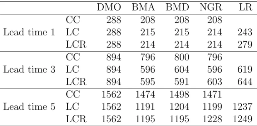
LCR ensemble adjustment schemes. . . 77 3.2 Brier scores for the CC, LC and LCR schemes at forecast lead times
1,3 and 5, evaluated at the 50% threshold. The climatology forecast score is 2500. . . 87 3.3 Brier scores for the CC, LC and LCR schemes at forecast lead times
1,3 and 5, evaluated at the 2% threshold. The climatology forecast score is 1960. . . 87 3.4 Brier scores for the CC, LC and LCR schemes at forecast lead times
1,3 and 5, evaluated at the 1% threshold. The climatology forecast score is 990. . . 87 3.5 The reliability component of the Brier score decomposition for
fore-cast lead times 1,3 and 5 at the 50% threshold. . . 91 3.6 The reliability component of the Brier score decomposition for
fore-cast lead times 1,3 and 5 at the 2% threshold. . . 91 3.7 The reliability component of the Brier score decomposition for
fore-cast lead times 1,3 and 5 at the 1% threshold. . . 91
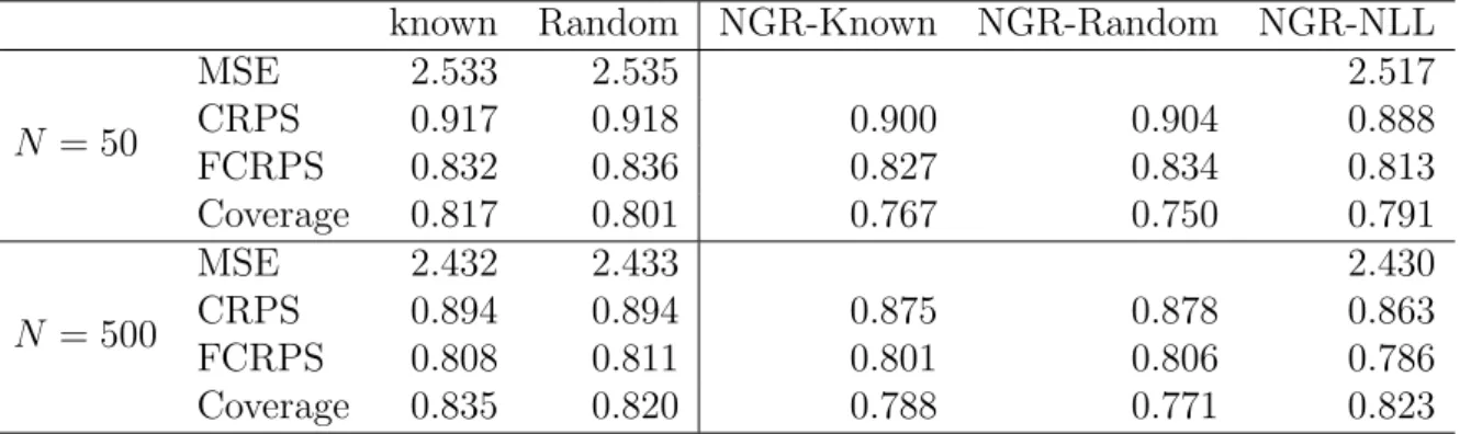
4.1 Results of the simulation study with parameters estimated from train-ing samples of size 50 and 500. Measures of the skill of deterministic forecasts (MSE) and ensemble calibration (CRPS, FCRPS and Cov-erage), for the two distribution-free post-processing methods (Known and Random), and ensemble forecasts sampled from NGR distribu-tions using the moment-based parameter estimates (NGR-Known and NGR-Random) and likelihood-based estimates (NGR-NLL). . . 125 4.2 Measures of the skill of deterministic forecasts (MSE) and
ensem-ble calibration (CRPS, FCRPS and Coverage) for the distribution-free and NGR post-processing methods with moment-based parame-ter estimates (Known and Random), and likelihood-based estimates (NLL), for post-processed ensemble forecasts in the Lorenz 1996 sys-tem. . . 129
4.3 Univariate scores for the raw ensemble forecasts, and ensemble fore-casts recalibrated with the distribution-free and likelihood-based NGR post-processing methods, at forecast lead times of 24 and 72 hours. The scores are averaged over the 17× 18 grid that approximately covers the UK. . . 132
5.1 Brier scores and the reliability (Rel) and resolution (Res) components of their decomposition, calculated at five thresholds of interest, for training samples of size N = 60. The Brier scores and the resolution components are scaled by 104, and the reliability components are scaled by 106. . . . 162
5.2 The CRPS for the raw ensemble forecasts, and ensembles sampled from plug-in and bootstrap BMA forecast distributions at Berlin, Frankfurt and Hamburg airports for the period 1 May 2010 – 30 April 2011. . . 167 5.3 The energy scores for the raw ensemble forecasts and ensembles
sam-pled from plug-in and bootstrap BMA forecast distributions for the spatial field defined by Berlin, Frankfurt and Hamburg airports, for the period 1 May 2010 – 30 April 2011. . . 168
2.1 Observations yas a function of the ensemble mean ¯xfor forecast lead times 1,3 and 5. A nonparametric estimate to the observations is shown in red. . . 66 2.2 Plots of the squared residualsr2as a function of the ensemble variance
s2 for forecast lead times 1,3 and 5. A nonparametric estimate to the expectation of the squared residuals is shown in red. . . 66
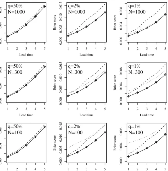
3.1 Brier scores as a function of lead time for the DMO (dashed), BMA (crosses), BMD (circles), NGR (solid) and LR (dotted) forecasts un-der the LC scheme at the 50%, 2% and 1% thresholds with parameter estimation performed with training samples of sizeN = 1000, 300 and 100. . . 89 3.2 Reliability diagrams at lead time 1 for BMA, BMD and NGR with
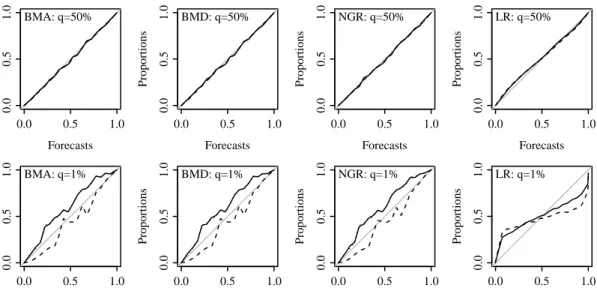
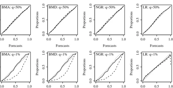
adjustment schemes CC (dashed), LC (dotted) and LCR (solid) for common and extreme thresholds, q. Also LR with η=a+bx (solid) and η =a+bx+ds2 (dashed). . . 90 3.3 As for figure 3.2 but for forecast lead time 3. . . 92 3.4 As for figure 3.3 but for forecast lead time 5. . . 92
4.1 Box and whisker plots for the parameter estimates ˆa,ˆb,ˆc and ˆd for the ‘known’ method (left), the measurement error method (middle) and the likelihood-based NGR estimates (right). . . 122 4.2 Rank histograms for the distribution-free post-processed ensemble
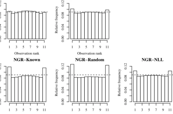
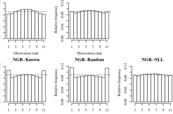
forecasts (top row), and ensemble forecasts sampled as equidistant quantiles from NGR distributions using the known, measurement er-ror, and NLL parameter estimates (bottom row). The training sam-ple size is N = 50. The horizontal lines indicate the bin heights of uniform histograms. . . 123 4.3 As for figure 4.2, but with training samples of size N = 500. . . 124 4.4 Rank histograms for the Raw ensemble forecasts, the two
moment-based, distribution-free post-processing methods (Known and Ran-dom), and ensemble forecasts sampled from NGR distributions using the moment-based and likelihood (NLL) parameter estimates. The forecast lead time is t= 3. . . 130
4.5 As for figure 4.4, for forecast lead time t= 5. . . 131 4.6 Multivariate rank histograms and energy scores (ES) for the raw
en-semble forecasts, the ‘known’ and ‘random’ forecasts post-processed with the distribution-free post-processing method, and forecasts sam-pled as equidistant quantiles from NGR forecast distributions with NLL parameter estimates, with and without ECC. Forecast lead times are 24 hours (left) and 72 hours (right). . . 134
5.1 Coverage of the 95% prediction intervals, the ignorance score (Ign) and the CRPS for the plug-in forecasts (open circles) and the predic-tive bootstrap forecasts (filled circles) as a function of training sample size, N, for simulated observations that follow the NGR model. . . . 155 5.2 PIT histograms for the plug-in NGR forecast distributions (left) and
bootstrap forecast distributions (right), for training samples of size
N = 30 (top row) and N = 60 (bottom row). . . 156 5.3 As for figure 5.1, but for observations that are distributed according
to the MOS statistical model. The results of the analytic forecasts are shown as open diamonds. . . 157 5.4 Coverage of the 95% prediction intervals, the ignorance score (Ign)
and the CRPS for the plug-in forecasts (open circles) and the predic-tive bootstrap forecasts (filled circles) as a function of training sample size, N, for probability forecasts of 2-metre temperature. . . 160 5.5 PIT histograms for probability forecasts of 2-metre temperature using
plug-in (left) and predictive bootstrap (right) forecasts. Model pa-rameters are estimated using rolling training samples of the previous 60 ensemble forecasts and observations. . . 161 5.6 As for figure 5.5, but for training samples of size N = 30. . . 162 5.7 Residualsrt as a function of the ensemble mean ¯xt. A nonparametric
Loess approximation to the expectation of the residuals is shown in red. . . 164 5.8 Squared standardised residuals ssrtas a function of the ensemble
stan-dard deviation st. A Loess approximation to the expectation of ssr is
shown in red. The vertical axis is plotted on a square root scale. . . . 165
6.1 Forecast residuals r as a function of ensemble mean ¯x. A nonpara-metric approximation to the expectation E(r) is shown in red. . . . 174 6.2 Squared standardised residuals ssr as a function of ensemble
stan-dard deviations. A nonparametric approximation to the expectation
E(ssr) is shown in red. The vertical axis is plotted on a square root scale. . . 175
6.3 Squared standardised residuals ssr as a function of ensemble standard deviation s, for NGR forecast distributions with variance given by equations (6.1) and (6.3). A nonparametric approximation to the expectation E(ssr) is shown in red. The vertical axis is plotted on a square root scale. . . 177 6.4 Pit histograms for the standard NGR model (left) and the revised
model with variance given by equation (6.5) (right). . . 179 6.5 Rank histograms for ensemble forecasts whose members are
depen-dent. Observations are independent of the ensemble members (left), and share the same multivariate distribution (right). . . 183 6.6 The fair CRPS as a function of the model parameter b, for simulated
data and ensemble forecasts post-processed with equation (6.6). . . . 184 6.7 Rank histograms for simulated data and ensemble forecasts
Weather conditions have had wide-ranging effects on humanity, seemingly since the beginning of time. Most obviously, the weather is a crucial factor in determining crop yields, and adverse periods of weather can lead to humanitarian crises. In modern society, weather conditions have both social and economic impacts. For example, in recent years the United Kingdom has witnessed several instances of wide-spread flooding. These events have impacted upon the livelihoods of those affected, as well as posing new challenges to the insurance industry. Other businesses and industries that are sensitive to weather conditions include supermarkets, construction, ship-ping, aviation and tourism. Indeed, in recent times the economic significance of the weather has led to the development of financial instruments that can be purchased by businesses to hedge against, and thus limit their financial exposure to, adverse weather conditions.
With the above comments in mind, it is clearly desirable to be able to provide accurate forecasts of future weather conditions. The possibility of mathematical approaches to weather forecasting was recognised as long ago as 1922, in the founding work of Lewis Richardson, ‘Weather prediction by numerical process’. Since then, the advent of computers and supercomputers has given rise to weather forecasts over the entire planet, for many weather variables, for forecast lead times up to and beyond two weeks. Weather forecasts are primarily based on numerical models of the atmosphere, which are derived from the field of fluid dynamics.
Until the last decade, weather forecasts were almost always deterministic in nature. For example, a forecaster might state ‘The temperature at 12pm tomorrow will be 20◦C’. However, despite years of research and the computational power available to the forecasters of today, weather forecasts are still subject to errors, and so we can not treat such deterministic forecasts as exact predictions that can be wholly relied upon. The uncertainty in weather forecasting has provided an opportunity for statisticians to determine systematic errors in weather forecasts that can be corrected, as well as to quantify the uncertainty in such forecasts. In other words, recent developments have led to the field of probability weather forecasts, rather than deterministic weather forecasts. By quantifying the uncertainty in the deterministic forecasts that are typically issued, users of probability forecasts can also estimate
the likelihood of the occurrence of weather events. For example, local councils may wish to estimate the joint likelihood of temperatures falling below 0◦C and heavy rainfall, which would lead to the formation of ice. Such estimates can then be used to make risk-based decisions — in the given example, councils may choose to deploy road gritting services if the probability forecast of ice formation exceeds a certain threshold.
The uncertainty in weather forecasts of the future atmospheric state is based upon so-called ‘ensemble forecasts’. An ensemble forecast is a collection of deterministic forecasts that differ in either the numerical model used to issue the forecasts or the initial atmospheric conditions that are supplied to the model. As the constituent members of an ensemble forecast will typically differ in their forecast values, an ensemble forecast provides a means of estimating the probability of certain weather events. For example, if six of nine ensemble members forecast the temperature, T, to fall below 0◦C, then we could assign a probability forecast Pr(T ≤ 0) = 2/3. Furthermore, the width of the ensemble forecast (i.e. the difference in the largest and smallest member), could be used as an 80% prediction interval — that is, an interval within which we would expect temperature observations to fall 80% of the time in the long-run.
Unfortunately, however, ensemble forecasts do not provide reliable representations of the forecaster’s uncertainty in the future, unknown observations. This is due to per-sistent errors in the numerical models used for the ensemble member forecasts, and uncertainty in how to select initial conditions with which to initialise the numerical models. For example, operational ensemble forecasts are often underdispersed, and so issuing probability forecasts of an event by the proportion of ensemble members that predict its occurrence leads to inaccurate probability forecasts — in the above example, the event{T ≤ 0}, which was assigned probability 2/3, will typically not occur on two thirds of occasions. Similarly, the prediction intervals of operational ensemble forecasts are often too narrow, and so the verifying observations lie outside the intervals more often than one would like. This has led to the development of the field of so-called ‘ensemble post-processing’, which is the subject of this thesis. En-semble post-processing methods can be thought of in two classes. Firstly, enEn-semble forecasts may be corrected, for example by the removal of systematic errors in the en-semble location and spread. The output from the post-processing method is another ensemble forecast, which (we should hope) has more desirable properties than the initial, so-called ‘raw’ ensemble forecast. Alternatively, and more commonly used in practice, is to use information contained in ensemble forecasts to issue probability forecasts, usually in the form of probability distributions. For example, a popular post-processing method that we use frequently throughout this thesis is to model the verifying observation as a Gaussian-distributed random variable, where the
ex-pectation and variance of the Gaussian distribution are modelled as linear functions of the sample mean and sample variance of the ensemble forecast. Well-known prop-erties of the Gaussian distribution can then be used to issue probability forecasts and prediction intervals, as well as deterministic forecasts. For example, the expec-tation of the Gaussian probability forecast distributions has frequently been shown to be a more accurate deterministic forecast than either the individual ensemble members or the ensemble mean, while the interval bounded by the 100×α/2% and 100×(1−α/2)% quantiles, where α is a constant in the interval (0,1) provides a 100×(1−α)% prediction interval. Ensemble post-processing methods are typically statistical models, and provide an opportunity for novel applications of statistical methods. In this thesis we present work that tackles several problems in the field of ensemble post-processing using statistical methodology.
The remainder of this thesis is organised as follows. In chapter 2 we give a broad ex-position of the background material that we make use of in later chapters. The chap-ter begins with an overview of ensemble forecasting, including early development and current operational practice. We then give a detailed introduction and discussion of ensemble post-processing methods, many of which we make use of in our new work. The chapter concludes with an overview and discussion of the various meth-ods that we use for the verification of both deterministic and probability forecasts, and a description of the datasets that we use in exemplifying our new methodology. In chapter 3 we present an investigation into ensemble post-processing methods for extreme events. We illustrate that allowing additional flexibility in the statistical models used for ensemble post-processing produces significant improvements to the skill of probability forecasts of the form Pr(y≤q), wherey is the verifying observa-tion, andq is anextreme threshold of interest. This work has been published in the literature [Williams et al., 2014]. In chapter 4 we introduce a novel post-processing method that leads to recalibrated ensemble forecasts, rather than probability fore-casts. Our new method makes fewer assumptions than are usually required, and serves as a more useful baseline than the simple frequency-based approaches de-scribed above. We recommend that new ensemble post-processing methods should seek to improve upon our baseline method. In chapter 5 we address the issue of uncertainty in the parameter estimates of the statistical models used for ensemble post-processing, a topic that was hitherto largely neglected in the literature. The results presented have also been published [Siegert et al., 2015a]. We show that prob-ability forecasts issued by ensemble post-processing methods are more reliable when they account for parameter uncertainty, and we propose a method of doing so that is easy to implement. Finally, in chapter 6, we introduce two ideas that we think worthy of further research. We illustrate how diagnostic plots, which are widely used in statistical modelling but are infrequently discussed in the post-processing literature, can be used to improve the specification of the statistical models issued
by ensemble post-processing methods. We then discuss the effect of dependencies between ensemble members, expressed through their correlation, on the conclusions that we may draw from commonly employed verification measures of forecast skill. Chapter 6 concludes with a summary of our findings presented during the thesis, and suggests directions for future research.
and ensemble post-processing
2.1 Introduction
In this chapter we provide details of much of the material that forms the basis for our novel work presented in chapters 3–6. The chapter is organised as follows. In section 2.2 we provide a brief overview of numerical weather prediction, and give an outline of the methodology that is used in operational ensemble weather forecasting. In section 2.3 we discuss the notion of calibration for both probability and ensemble forecasts, in particular, what is meant by ‘reliability’, ‘resolution’ and ‘forecast uncertainty’. In section 2.4 we provide an extensive review of many ensemble post-processing methods, several of which we make use during this thesis. We also give details of the routines that are used for estimating the parameters in the statistical models that are specified by ensemble post-processing methods. In section 2.5 we provide details of the graphical and quantitative methods that we use for the verification of out-of-sample forecasts in our new work, for both probability and ensemble forecasts. Finally, in section 2.6 we describe the datasets that are used to illustrate our new contributions in chapters 3–6.
2.2 Numerical weather prediction and ensemble
weather forecasting
2.2.1 Introduction
In this section we provide a brief overview of the main components of an ensem-ble forecasting system. We begin with a discussion of numerical weather prediction (NWP) models, and explain the main sources of error that result from the many dif-ficulties in constructing accurate models of the atmospheric state. In section 2.2.3 we introduce the practice of ensemble forecasting, which provides a means of
acknowl-edging and accounting for the aforementioned errors in the deterministic forecasts that are issued by NWP model forecasts. We recommend the text Kalnay [2003] for a far more detailed and complete exposition of the material that is presented in these two subsections. We conclude this section with a discussion of two interpretations of ensemble forecasts that are commonly employed by forecasters.
2.2.2 Numerical weather prediction
The twentieth century saw the rapid development of machines that were able to automate mathematical operations, which grew in to the computers and super-computers of today. These technological advances gave rise to the possibility of completing tasks that required large numbers of calculations for the first time. Not least among these was the ability to use numerical models of the atmosphere to issue meteorological forecasts. Prior to such an automated approach, the first at-tempts at weather forecasting (Richardson 1922, see Richardson [2007]) involved the laborious process of making calculations by hand and interpolating observations gathered at weather stations to an appropriate grid. While much of the fundamental process established by Richardson (and others) remains to this day, powerful com-putation allows high resolution forecasts to be automatically generated for multiple meteorological variables, forecast lead times and for increasingly fine grids in three dimensional space.
Modern-day operational weather forecasts are based on numerical weather predic-tion (NWP) models, which are an approximapredic-tion to the physics of the atmosphere. The models are derived from the field of fluid dynamics, and take the form of a high-dimensional system of coupled partial differential equations (PDEs). These PDEs represent the evolution in time and the spatial dependence of the many meteorolog-ical variables comprised within the model, including the complicated relationships governing inter-variable interactions. Initially based on a small set of equations that approximated the most important properties of the dynamics of the atmosphere, known as the ‘full equations of motion’, years of research has seen NWP models develop in to high-dimensional systems that are used operationally for forecast lead times of two weeks and beyond. The models provide approximations to large-scale, slowly-varying features, such as the Atlantic jet stream, as well as to small-scale, localised phenomena such as cloud formations and associated localised precipitation. Historically, a deterministic weather forecast was issued as the output of a single run of an NWP model. However, due to the many difficulties in numerical weather prediction, these forecasts are imperfect. In the remainder of this subsection we discuss three of the most difficult areas of numerical weather prediction, each of which lead to errors in the deterministic forecasts that are issued.
As is the case for all dynamical systems, NWP models are initial value problems, in the sense that their evolution through time is dependent on the initial value supplied. When making a single, deterministic weather forecast, therefore, it is important that the initial condition supplied to the model is the best available estimate of the atmospheric state at that time. This estimate is known as the analysis, and is produced using one of a variety of methods from the field of data assimilation. Errors in the analysis forecast will therefore lead to errors in the resulting deterministic forecast, even in the idealised setting of a ‘perfect’ NWP model. In his founding work in the 1960s [Lorenz, 1963, 1965], Lorenz studied the temporal evolution of models that were perceived as realistic approximations to the atmosphere at the time. In a series of numerical experiments, Lorenz found that two runs of an idealised model started from initial conditions that differ only very slightly will, after sufficient time, appear to evolve independently of one another, as they might had the two model runs been started from very different initial conditions. This problem became known as the ‘butterfly effect’, which considered the effect of small disturbances (or perturbations) in the initial conditions on the long-run evolution of dynamical models. In terms of the predictability of the atmosphere, Lorenz suggested that even a perfect NWP model would lose all predictive skill for forecast lead times longer than approximately two weeks, due to errors in the initial conditions which, even if known perfectly, are subject to round-off when used as inputs to computer models. Analogously, small differences in the analyses issued by weather centres could result in markedly different forecasts, even with the use of a common NWP model. There is yet to be a unified approach to producing analyses and, therefore, model initial conditions are likely to differ across operational centres. Furthermore, Lorenz found that the predictability of nonlinear dynamical systems with instabilities, such as the atmosphere, is dependent on the state of the system itself — the system is more stable in certain states than in others and, therefore, the skill of NWP forecasts is likely to vary, depending on the atmospheric stability at the time.
Secondly, constructing accurate representations of the atmospheric physics is a highly complicated task, and one that even after many years of research is still problematic. Large-scale features are generally well understood and are therefore predictable, while small-scale phenomena remain problematic. In addition, under-standing the complicated interactions between the various features of the planet, for example the differences in the behaviour of the atmosphere over the oceans and over land, and then casting these interactions in a viable mathematical form is a complicated research problem. Furthermore, NWP models must be ‘tuned’ to the observed atmosphere by adjusting the many parameters that control their evolution as specified by the aforementioned coupled system of PDEs.
Finally, approximating the solution of the NWP model, that is, the system of PDEs that describe the atmospheric physics and structure, is a highly complicated task. Due to the size and complexity of the system of PDEs, closed-form solutions are not available. It is therefore necessary to discretise the model and use numerical methods to approximate the model solution. It is necessary to discretise the model over a fixed grid, the structure of which forms a research problem in its own right. Popular choices of grid coordinates include Cartesian, Spherical and Gaussian. The model resolution refers to the density of grid points, with finer grids corresponding to models with higher resolution. The temporal evolution is also discretised, such that the model state is estimated at discrete, rather than continuous time steps. With the model suitably discretised, numerical methods, known as finite difference schemes, can be applied to estimate the model state at each gridpoint and time step. The choice of numerical scheme has considerable implications, not only in terms of the accuracy of the model solution, but also computational cost. The development of improved numerical methods is also an important field of research in its own right, and further discussion of this topic is beyond the scope of this thesis.
As mentioned above, NWP models typically provide accurate representations of large-scale features, while forecasters are less confident in their ability to represent localised events. The difficulty in predicting small-scale features is largely due to the fact that they occur within areas smaller than the ‘grid boxes’ that are enclosed by the grids on which NWP models are based. Inaccuracies in initial conditions and imperfect model physics, as well as the difficulties in approximating the solution of the model itself, all contribute to the inaccuracies that are observed in operational weather forecasts.
2.2.3 From deterministic forecasts to ensemble forecasts
In the previous subsection we highlighted several sources of uncertainty in the fore-casts issued by NWP models:
• The sensitivity of the NWP model to the initial conditions, and consequently the effect of analysis error on the model evolution.
• Uncertainty in the physical parameterisations and the parameter values used. • The loss of accuracy in the model solution due to the discretisation of the
model over space and time.
• The stability of the atmospheric system itself — Lorenz showed that the pre-dictability of unstable dynamical systems can vary.
Considering these fundamental problems of weather prediction in combination, there-fore, forecasters are rightly uncertain as to the accuracy of the deterministic forecasts that are issued by NWP models. It is therefore natural to turn to a framework that enables a forecaster to both issue a deterministic forecast and to provide an as-sessment of their confidence in that forecast or, or in other words, to quantify their forecast uncertainty. The framework for quantifying forecast uncertainty is therefore probabilistic in nature. A more detailed discussion of forecast uncertainty is pro-vided in section 2.3. In this subsection we provide an overview of ensemble weather forecasting, which is the framework upon which forecast uncertainty is based.
As described in chapter 1, an ensemble forecast is a collection of deterministic fore-casts that, in general, differ in their forecast values. We define an ensemble forecast for a general forecast occasion as x = (x1, x2, . . . , xM), where M denotes the
num-ber of ensemble memnum-bers, or the ensemble size. We now provide a brief overview of the history of ensemble forecasting, and describe the methods that are commonly employed in their generation.
Epstein [1969] proposed the idea of a so-called ‘stochastic-dynamic’ framework for weather forecasting. Epstein’s idea was to develop a partial differential equation that approximated the evolution of a probability density function (PDF) for the future, verifying observation, based on NWP model forecasts. The idea was to sample the possible initial conditions, and to approximate this PDF with the resulting model runs. The approach involved a very large number of model runs, which proved computationally infeasible. Even after some simplifying assumptions to estimate the first two moments rather than the entire PDF, Epstein’s approach was not applicable in settings beyond those of low-dimensional, ‘toy’ models.
Hoffman and Kalnay [1983] experimented with so-called ‘lagged average forecasting’, which generates ensemble forecasts whose members are deterministic forecasts of the same verifying observation, but initialised at different times. While the method obviates the need to generate perturbations to the initial conditions, it is necessary to weight the ensemble members according to their age, to accommodate the idea that their forecast skill will decrease with increasing lead time. Obtaining the ensemble member weights requires estimating the temporal evolution of the covariance matrix of forecast errors, and difficulties in doing so have resulted in limited applications of the method. There are also limitations on the size of ensembles that can be generated from lagged average forecasting, as large ensemble forecasts would require the inclusion of forecasts at prohibitively long lead times.
Leith [1974] introduced the ‘Monte Carlo’ approach to ensemble forecasting. The idea is to generate ensemble forecasts by perturbing the analysis, and using these perturbed analyses as initial conditions for the NWP model forecasts. The
pertur-bations are sampled at random from a multivariate distribution that is based upon the dependence structure of historical forecast errors and scaled such that their am-plitude is equal to the estimated analysis error. The dependence structure is derived in the data assimilation cycle, and must reflect the statistical horizontal and verti-cal structure of the forecast errors. Among other findings, Leith showed that the ensemble mean of Monte Carlo ensemble forecasts is in general a more skilful deter-ministic forecast than the ‘control forecast’, the NWP model forecast initialised at the analysis.
An alternative but related approach to Monte Carlo ensemble forecasting is to choose perturbations that are not sampled at random, but instead include information that is pertinent to the current predictability of the atmosphere. This approach recognises Lorenz’s finding that the stability of the atmosphere, and therefore its predictabil-ity, is subject to variation. In this approach, the amplitudes of the perturbations depend on the estimated analysis errors at that time, which vary in keeping with the predictability of the atmosphere. Larger perturbations are chosen for more difficult forecasts, and smaller perturbations are used when atmospheric conditions are more stable. This is in contrast to the approach of Monte Carlo forecasting, for which initial conditions are chosen at random and so do not contain information about the current predictability of the atmosphere.
So-called ‘bred vectors’ are commonly used to generate perturbations that contain current information for the atmospheric stability. After first initialising ensemble members with randomly sampled initial conditions, as in the Monte Carlo approach, the evolution of the ensemble members is updated by adding regular (for example, every six hours) perturbations that depend on the forecast errors of the NWP model at that time. Bred vectors are commonly employed in operational centres [Kalnay, 2003, chapter 6]. It is reported (see section 6.6.2 of Kalnay [2003]) that experiments conducted at the National Centre for Environmental Prediction (NCEP) demon-strated that the second type of perturbation grew much faster than the perturba-tions that were chosen for Monte Carlo ensembles, resulting in ensemble forecasts that exhibited greater spread.
Two further approaches to producing ensemble forecasts are to use multiple data assimilation systems [Houtekamer et al., 1996] and to combine forecasts from mul-tiple operational centres [Hou et al., 2001]. In the former system, random noise is added to the observations to reflect uncertainty in the analyses, and the NWP model parameterisations are also perturbed. The idea behind the system is that perturbing the NWP model will increase the extent to which the main contributory sources of uncertainty described in the previous subsection are sampled. In the sec-ond approach, the authors suggest that the forecast uncertainty will be well sampled by combining the analyses and state of the art NWP models from multiple weather
centres, whose NWP models and data assimilation processes are likely to differ.
2.2.4 Interpretations of ensemble forecasts
As mentioned in section 2.2.3, ensemble forecasts have been used successfully to im-prove the skill of deterministic forecasts and to estimate the associated forecast un-certainty. Other desirable applications include estimating the probability of binary events, such as the probability that the temperature will exceed a given threshold on a given day or, in a multivariate setting, that precipitation will exceed a certain threshold and the temperature will fall below 0◦C, resulting in the likely formation of ice. As described in the previous chapter, a related application is the estimation of prediction intervals for the verifying observations.
With a variety of possible applications, therefore, there is evidently a need for clarity over how exactly to interpret the ensemble forecasts. For example, if a forecaster wishes to derive probability forecasts from ensemble forecasts produced using the lagged average forecasting scheme mentioned in section 2.2.3, it appears unnatural to assign equal importance, or weight, to the ensemble members, given we know that the forecasts differ in age and, consequently, that some members are likely to be more skilful than others. On the other hand, assigning equal weight to all members appears more acceptable in the Monte Carlo setting, where perturbations to the analysis at the forecast initialisation time are simulated randomly. Equally, the forecaster may need to think carefully when handling ensemble forecasts whose members differ due to perturbations in the NWP model and/or the initial condi-tions. We may expect those ensemble members issued with perturbed NWP model parameterisations to produce less skilful deterministic forecasts than the control forecast, given that the parameters of the NWP model are likely to be ‘tuned’ based on the control forecast.
From a practical perspective, it is often necessary for the forecaster to make a simplifying assumption when drawing inferences from ensemble forecasts or, in other words, to decide upon an interpretation of the ensemble members. One commonly employed interpretation is that the ensemble members represent an independent and identically distributed (IID) sample from an underlying probability distribution. For the remainder of this thesis we refer to this distribution as theensemble distribution. Analogously, the verifying observation for an individual forecast occasion can be viewed as an IID draw from an underlying distribution, hereafter referred to as the observation distribution. As mentioned in the introductory chapter, a desirable property of an ensemble forecasting system is that the ensemble distribution, of which the ensemble forecast can be interpreted as representing a sample, and the observation distribution are equal.
The members of ensemble forecasts that we know, or choose to interpret as IID draws from an underlying distribution are said to be exchangeable. Furthermore, ensemble forecasts whose members are dependent, but can be viewed as a single draw from a symmetric multivariate distribution are also exchangeable. For example, an assumption of exchangeability is reasonable if a single NWP model is used and initial conditions are generated in a consistent manner, such as by random perturbations to the analysis. This leads to the following definition.
Definition 2.2.1 The members of an ensemble forecast x = (x1, x2, . . . , xM) are
exchangeable if the statistical properties of x are invariant to any relabelling of its constituent members. In other words, the members of an ensemble forecast are exchangeable if the forecaster is able to treat all ensemble members as statistically indistinguishable.
A second interpretation of an ensemble forecast is that its empirical distribution function (EDF) represents a probability forecast distribution for the verifying ob-servation, y. In this case the probability forecast distribution of y, conditional on the ensemble forecastx, is
F(y|x) = 1 M M ∑ m=1 I(xm ≤y), (2.1)
where F(y) denotes the cumulative distribution function (CDF) for y, and I(·) is the indicator function that takes the value 1 if its argument is true, and 0 if its argument is false. Equation (2.1) assumes equal weighting between ensemble members. Alternatively, the distribution fory could be constructed using weighted ensemble members such that
F(y|x) = M ∑ m=1 wmI(xm ≤y) where M ∑ m=1 wm = 1,
and an appropriate statistical framework is needed to estimate the weights wm,
for m = 1,2, . . . , M. In section 2.5 we discuss how different interpretations of the ensemble members can affect how the skill of ensemble forecasts is assessed.
2.3 Forecast calibration and forecast uncertainty
2.3.1 Calibration for probability forecasts
As we describe in the next section (2.4), forecasters often use ensemble forecasts as a basis for issuing probability forecasts of the future, unknown atmospheric state. Depending on the nature of the predictand (the meteorological variable for which probability forecasts are issued), forecasters may issue continuous probability fore-cast distributions, discrete (either binary or categorical) distributions or, in a few special cases, a discrete-continuous mixture distribution. Probabilistic forecasters are particularly interested in two distinct properties of their forecasts, namely the forecast reliability, or calibration, and the forecast resolution. Forecast reliability refers to the ability of a probabilistic forecasting system to issue ‘accurate’ proba-bility forecasts, in the sense that the value or event that materialises occurs with the relative frequency expected by the probabilistic forecasting system. Forecast resolution, meanwhile, is a measure of the information content of a forecast. The resolution can be viewed as the variability of the verifying observations, conditional on the probability forecasts. Forecasts with high resolution provide useful informa-tion to the forecast user, and so the condiinforma-tional variability of the observainforma-tions is large. On the other hand, forecasts with no resolution are unable to distinguish between the possible outcomes of the observations, and so there is no (conditional) variability in the observations. The notions of reliability and resolution are perhaps best exemplified with a discussion of probability forecasts of binary events, which now follows.
Let q denote a threshold of interest, and y the verifying observation, where y is unknown when the forecast is issued. Suppose the forecaster issues forecasts of the binary event z = I(y ≤ q), which take the form p = Pr(y ≤ q) = Pr(z = 1). A probabilistic forecasting system for z is reliable if, among those occasions on which the event z = 1 is forecast to occur with probability p, the event does occur with relative frequencyp, and this is true for allp. The forecast resolution of this system is a measure of its ability to distinguish between the outcomes z = 0 and z = 1. Observe that the constant forecast p = ¯z is reliable — the long-run proportion of events that satisfy z = 1 is equal to the probability forecast p — but the forecast has no resolution — it does not tell the user anything that cannot be inferred from historical observations. In section 2.5.5 we provide expressions for two measures that are commonly employed to assess the reliability and resolution of probability forecasts of binary events.
A further property of probabilistic forecasts that is of interest is known as the ‘sharp-ness’, which provides a measure of the dispersion of the probability forecasts. The
sharpness of forecasts for binary predictands, z, is often measured as the variance of the Bernoulli distribution with probability p = Pr(z = 1), given by p(1−p). Similarly, the sharpness of forecasts for continuous predictands is often measured as the variance of the continuous forecast distribution. Forecasters prefer probability forecasts that are both reliable and sharp. In this thesis we refer to the guiding principle of Gneiting et al. [2007] and other papers by the same authors, who state that forecasts should be as sharp as possible, subject to reliability. Specifically, in a discussion of desirable properties of probability forecast distributions for continuous predictands, Gneiting et al. state: “The more concentrated the forecast PDF, the sharper the forecast, and the sharper the better, subject to calibration.”
In this thesis we also make use of ‘prediction intervals’, which provide an insight in to both the sharpness and calibration of probability forecasts for continuous, rather than binary, observations. For a given probability forecast distribution, we define the α% prediction interval as the interval within which the verifying observation lies with probability α. For example, for a Gaussian forecast distribution a 90% prediction interval for the verifying observation could be calculated as the interval (q.05, q.95), where the notationqβ refers to the β-quantile of the forecast distribution.
The ‘coverage’ of prediction intervals refers to the actual relative frequency of obser-vations that fall in such intervals. Prediction intervals for which the expected and observed coverage are not equal are indicative of probability forecast distributions that are not reliable. In keeping with the foregoing remarks concerning forecast reli-ability and sharpness, we would like prediction intervals to be as narrow as possible, subject to having accurate coverage.
We also make frequent use of the term ‘forecast uncertainty’ in the remainder of this thesis, the precise meaning of which depends on the context of the probabilistic forecast. For example, forecast uncertainty for a continuous predictand usually refers to the spread, or dispersion, of the probability forecast distribution, and can be viewed as a measure of uncertainty in deterministic forecasts that might also be inferred from the forecast distribution, such as its expectation or median. Forecasters are ‘more uncertain’ when issuing forecasts from probability distributions whose dispersion is large, compared with distributions whose dispersion is small. There are natural relationships between such forecasts and prediction intervals — prediction intervals are narrower for forecasts in which we are confident, or less uncertain.
2.3.2 Calibration for ensemble forecasts
Forecasters sometimes prefer to issue ensemble forecasts, rather than probability forecasts, and so it is also important to establish the notion of calibration for en-sembles. As described in section 2.2.4, ensemble forecasts can be interpreted as
either a probability forecast for the verifying observation (via their EDF), or as a collection of IID realisations from an underlying ‘ensemble distribution’. In the for-mer case the comments given in the previous subsection apply. On the other hand, we view ensemble forecasts whose members are IID samples as being calibrated with the verifying observations if the observations also appear as IID realisations of the corresponding ensemble distributions.
Calibrated ensemble forecastsx= (x1, x2, . . . , xM) for continuous predictands, whose
members are IID random draws, have the following appealing properties. The ex-pectation of the ensemble mean, ¯x, is equal to the expectation of the observation,y, that isE(¯x) = E(y). Secondly, the range of the ensemble forecast, max(x)−min(x), forms a 100×(M −1)/(M + 1)% prediction interval with the correct long-run ob-served coverage.
Historically, and (we understand) still in some operational settings, the empirical distribution functions (EDFs) are used as probability forecast distributions for the verifying observations. For example, the EDF of an ensemble forecast might be used to issue a probability forecast for a binary predictand by calculating the frequency of ensemble members that predict the event to occur. As we discuss in section 2.4.2.1, however, probability forecasts derived from such frequency-based approaches have undesirable properties, even if the ensemble forecast is calibrated with the verifying observation in the sense described above.
2.4 An overview of ensemble post-processing
methods
2.4.1 Introduction
While considerable effort has been devoted to the production of NWP models that accurately describe the physics of the atmosphere, as well as to the development of perturbations to the analysis that accurately represent the forecaster’s uncertainty of the atmospheric state at the model initialisation time, it remains the case that the evolution of the atmosphere is insufficiently resolved, and that the growth of the perturbations does not accurately reflect the state-dependent predictability of the atmosphere. Often the growth rates of the perturbations are slower than the growth rates resulting from the instabilities of the true atmospheric flow, and therefore many operational ensemble forecasts are underdispersed [Hamill and Colucci, 1997, 1998].
forecasts as a basis for stating their beliefs about their uncertainty in the future verifying observations. Persistent errors, or biases, in the location (the forecast values of the deterministic ensemble members) and the spread of ensemble forecasts mean that, for example, the proportion of ensemble members that forecast the occurrence of an event, such as the binary event{y≤q}, where yis an observation andqa threshold of interest, is not a reliable estimate of the probability of the event occurring. Typically the event will occur with relative frequency that is not equal to the proportion of ensemble members that predict it to do so or, in other words, ensemble forecasts are typically not well calibrated with the verifying observations. Similarly, prediction intervals, usually defined as the range of the ensemble forecasts (see section 2.3.2), are frequently too narrow — observations typically fall outside of the range of the ensemble forecasts more often than indicated by the nominal coverage of the prediction intervals.
Despite their deficiencies, however, ensemble forecasts often contain useful informa-tion that can be exploited to issue recalibrated forecasts of the future atmospheric state, either as probability forecasts or ensemble forecasts. For example, from as early as Leith [1974], the ensemble mean has frequently proven to be a more skilful deterministic forecast than the control forecast. Furthermore, the ensemble spread, which is usually measured by its sample variance, is often a useful predictor of the error in the ensemble mean forecast, despite the underdispersion typically observed; see, amongst many others Hamill and Colucci [1997, 1998]; Raftery et al. [2005]; Gneiting et al. [2005]. In other words, referring to our discussion in section 2.3.2, the ensemble variance is often a useful predictor of the forecast uncertainty. Ensem-ble forecasts with this property are said to exhibit ‘spread-skill relationships’. En-semble forecasts with large spread are often associated with enEn-semble means whose deterministic forecasting errors are larger than ensemble forecasts with small spread. Such spread-skill relationships are exploited frequently throughout this thesis.
As mentioned in chapter 1, ensemble post-processing methods often take the form of parametric statistical models that seek to quantify relationships (such as the bias) between the ensemble forecasts and observations, and specify probability forecast distributions for the future (unknown) verifying observations. However, an ensemble post-processing method could be as simple as, for example, removing a constant bias from each member. In this thesis we class any method that exploits relationships between the ensemble forecasts and observations to produce recalibrated forecasts as a post-processing method, whether in the form of probability forecast distributions or recalibrated ensemble forecasts. For example, in chapters 3 and 5, we investigate post-processing methods that construct continuous probability forecast distributions in the standard parametric statistical modelling framework, while in chapter 4 we introduce a new post-processing method that recalibrates ensemble forecasts only.
As is generally the case in statistical modelling, the majority of ensemble post-processing methods require the estimation of model parameters. These estimates are obtained from samples of historical ensemble forecasts and their verifying observa-tions, which we refer to as ‘training samples’ throughout this thesis. The parameter estimation procedure is usually performed by optimising an objective function that is calculated over the training sample, as in chapters 3, 5 and 6, using numerical algorithms to find the optimal set of parameter estimates. Alternatively, parameter estimates are sometimes calculated directly using techniques such as the method of moments, as in chapter 4. So-called ‘rolling’ training samples are often employed to estimate model parameters for the next forecast occasion — that is, a training sample of the N previous ensemble forecasts and verifying observations is used to estimate the parameters for the next ‘out-of-sample’ forecast.
Having obtained parameter estimates from a training sample of ensemble forecasts and observations, the chosen ensemble post-processing method can be used to is-sue either probability forecasts or post-processed ensemble forecasts (depending on the post-processing method) of the future, unknown atmospheric state or, in other words, to issue out-of-sample forecasts. We make clear this distinction by denoting out-of-sample forecasts and observations with the subscript t, and within-sample forecasts and observations (that are used for parameter estimation) with the sub-script i. The size of training samples is denoted by N, and the size of the dataset of out-of-sample forecasts is denoted by T. If a rolling training sample is used for parameter estimation, the parameter estimates will change with forecast occcasion
t, where t = 1,2, . . . , T indexes the out-of-sample forecasts in the test dataset. In certain studies, however, such as that presented in chapter 3, the same parameter estimates are used for each out-of-sample forecast. We make clear the distinction in our notation for the particular study at hand.
The remainder of this section is organised as follows. In section 2.4.2 we describe some simple methods for issuing probability forecasts for the binary event{yt≤q},
where q denotes a threshold of interest, that are related to the frequency-based approaches mentioned previously. In sections 2.4.3 and 2.4.4 we review several post-processing methods that were used in the publication Williams et al. [2014]. These post-processing methods, or adaptations thereof, have been successfully applied to a variety of problems in the forecasting of various meteorological variables, and are frequently used in chapters 3–6. We give an overview of the methods only, and defer more technical material such as the objective functions used for parameter estimation until they are required in chapter 3. In section 2.4.5 we outline some post-processing methods that tackle meteorological variables of renowned difficulty, such as wind direction and precipitation, and describe an extension to the logistic regression model described in section 2.4.4.3. We also outline some post-processing
methods that yield forecasts of multivariate quantities. We have not made use of many of the methods in section 2.4.5, either because we were not aware of them, they were not published until the later stages of the study, or they were not relevant due to being targeted at specific variables that were not under consideration. In section 2.4.6 we describe the approach of ensemble copula coupling (ECC), which is an increasingly popular method for producing post-processed ensemble forecasts of multivariate predictands, such as for spatial fields. Finally, in section 2.4.7 we give details of the procedures used in our work for the estimation of model parameters. We describe two popular objective functions and the numerical algorithms that are used to find the optimal parameter estimates.
2.4.2 Ad-hoc post-processing methods
2.4.2.1 Frequency-based probability forecasts
In this section we describe some simple frequency-based approaches for estimating probability forecasts of binary events. The climatology serves as the simplest prob-ability forecast of the formp= Pr(yt≤q), where q is a threshold of interest to the
user. The probabilityp is estimated from the empirical distribution function of the observed climatology as Pr(yt ≤q) =Fclim(q) = 1 N N ∑ i=1 I(yi ≤q), (2.2)
whereyi, i= 1,2, . . . , N denoteN historical observations. The climatology forecast
is reliable in the sense described in section 2.3.1, but has no resolution — the same forecast is always issued, and so does not provide any useful information to the user beyond that that can be inferred from the historical observations.
Until the growth in popularity of more sophisticated methods, probability forecasts of the form Pr(yt ≤ q) were derived from ensembles using simple frequency-based
calculations. These approaches are based on the assumption that the ensemble mem-bers are sampled from the ‘true’ probability density function (PDF) of the future verifying observationyt. In this case, the proportion of ensemble members
predict-ing the event {yt ≤ q} is a consistent and unbiased estimator of the probability of
the event occurring. In the simplest case, the proportion of members of the ensem-ble forecast xt = (x1,t, x2,t, . . . , xM,t) predicting the event {yt ≤ q} can be used to
estimate Pr(yt≤q) Pr(yt ≤q) = 1 M M ∑ m=1 I(xm,t ≤q). (2.3)
This probability forecast suffers from the implications that probability forecasts of 0 (1) are issued when the thresholdq is smaller (larger) than all ensemble members. An alternative estimator is
Pr(yt≤q) = Rank(q)t/(M + 1), (2.4)
where Rank(q)t=
∑M
m=1I(xm,t ≤q) + 1 is the rank of the threshold q when pooled
together with the members of the ensemble forecast xt. Again, however, this
esti-mator implies a probability of 1 when all ensemble members are smaller thanq, i.e. when Rank(q)t =M + 1.
Direct model output (DMO) is a further frequency-based estimator, that avoids probability forecasts of 0 or 1. Probability forecasts are given by
Pr(yt≤q) =
Rank(q)t−1/3
M+ 1 + 1/3 . (2.5)
Unlike the other frequency-based approaches described previously (equations (2.3) and (2.4)), the probability forecasts returned by equation (2.5) do not attain either the undesirable values of 0 or 1. The probability forecasts can range from 2/(3M+4) (when Rank(q)t = 1) to (3M + 2)/(3M + 4) (when Rank(q)t = M + 1). The
adjustments −1/3 to the numerator and 1/3 to the denominator of equation (2.5) are one of several possible corrections to frequency-based approaches, such as those given in equations (2.3) and (2.4). Wilks [2006b, page 41] provides several other possibilities. We have chosen to show the DMO forecasts as they were used in the article by Wilks [2006a] and in our own work presented in chapter 3.
Note that the four methods of issuing probability forecasts Pr(yt ≤q) described in
this section should not be viewed as ensemble post-processing methods, since the forecasts are simply a function of the members of the ensemble forecast xt — the
ensemble is not post-processed, and the probability forecasts are independent of any historical ensemble forecasts.
2.4.2.2 Rank histogram recalibration
As highlighted in section 2.4.1, in practice ensemble forecasts suffer from biases in both their location and dispersion. This was discussed by Hamill and Colucci [1997] in an application to probability forecasts of precipitation. Hamill and Colucci [1997, 1998] proposed an ensemble post-processing method that we refer to as rank histogram recalibration (RHR), that attempts to account for the biases in ensemble location and dispersion. Unlike the frequency-based approaches described above, the RHR method makes use of historical training samples of ensemble forecasts
and observations as follows. Firstly, constant biases are removed from the ensemble forecastsxi, i= 1,2, . . . , N, to form bias-corrected ensemblesxbi, where
b xim =xim+ 1 M ×N N ∑ i=1 M ∑ m=1 (yi−xim), for i= 1,2, . . . , N and m= 1,2, . . . , M, (2.6) so that the unconditional (over the entire training sample) sample mean of the bias-corrected ensemble members is equal to the sample mean of the observations
yi, i= 1,2, . . . , N. Then define a vector of weights,
wj = 1 N N ∑ i=1 I(Rank(yi) = j) forj = 1,2, . . . , M + 1 (2.7) where Rank(yi) = 1 + ∑M
m=1I(ˆxim≤yi) is the rank of the observation when pooled
together with the members of the (de-biased) ensemble forecast ˆxi. The weights are
therefore given by the relative frequency of the M + 1 possible ranks that can be taken by theN observationsyiover the training sample. This enables out-of-sample
probability forecasts to be issued, as we now describe.
Firstly, any constant bias is removed from the out-of-sample ensemble forecast xt,
using the same bias correction as was performed for the ensemble forecasts in the training sample. We then define the order statistics for the corrected ensemble fore-cast ˆxt, denoted ˆx
(m)
t for m = 1,2, . . . , M, such that ˆx (1) t <xˆ (2) t < . . . < xˆ (M) t . The
probability forecast distribution issued by the rank histogram recalibration method is then constructed as follows. The distribution is assumed uniform between con-secutive order statistics of the ensemble forecast, with each uniform distribution weighted by the relevant weight defined above. For example, the distribution be-tween ensemble members ˆx(1)t and ˆx(2)t is assumed uniform, and is weighted by w2,
and the uniform distribution between ensemble members ˆx(Mt −1)and ˆx(M)t is weighted bywM. The probability distribution for values that are unbounded by the ensemble
forecast must be specified by the forecaster. In an application to probability forecasts of quantitative precipitation, Hamill and Colucci [1997] assumed that observations
yt were uniformly distributed between 0 and the smallest ensemble member, ˆx (1)
t ,
but fitted a Gamma distribution to the right hand tail, that is used for probability forecasts of values that lie above the largest ensemble member, ˆx(Mt ). On the other hand, Wilks [2006a] fitted a Gaussian distribution to both tails of the RHR fore-cast distribution, with expectation and variance given by the ensemble mean and variance, respectively. Probability forecasts for observations in the lower and upper tails of the forecast distribution are weighted by w1 and wM+1, respectively. As
described earlier, many operational ensemble forecasts are underdispersed, and so a relatively large proportion of observations fall in the tails of the probability forecast distributions. We denote by gRHR(·) the parametric family of probability
distribu-tions that is chosen for the tails of the RHR forecast distribution, with cumulative distribution function GRHR(·). As with Wilks [2006a], this probability distribution
is typically dependent on the ensemble forecast ˆxt. The RHR forecast distributi