University of Windsor University of Windsor
Scholarship at UWindsor
Scholarship at UWindsor
Electronic Theses and Dissertations Theses, Dissertations, and Major Papers
9-12-2019
A Simple Approach to Generating Body Force Models of Jet
A Simple Approach to Generating Body Force Models of Jet
Engine Fans and its Application to Inlet-Fan Coupling Interaction
Engine Fans and its Application to Inlet-Fan Coupling Interaction
Quentin J. Minaker University of Windsor
Follow this and additional works at: https://scholar.uwindsor.ca/etd
Recommended Citation Recommended Citation
Minaker, Quentin J., "A Simple Approach to Generating Body Force Models of Jet Engine Fans and its Application to Inlet-Fan Coupling Interaction" (2019). Electronic Theses and Dissertations. 7821.
https://scholar.uwindsor.ca/etd/7821
This online database contains the full-text of PhD dissertations and Masters’ theses of University of Windsor students from 1954 forward. These documents are made available for personal study and research purposes only, in accordance with the Canadian Copyright Act and the Creative Commons license—CC BY-NC-ND (Attribution, Non-Commercial, No Derivative Works). Under this license, works must always be attributed to the copyright holder (original author), cannot be used for any commercial purposes, and may not be altered. Any other use would require the permission of the copyright holder. Students may inquire about withdrawing their dissertation and/or thesis from this database. For additional inquiries, please contact the repository administrator via email
A Simple Approach to Generating Body Force
Models of Jet Engine Fans and its Application to
Inlet-Fan Coupling Interaction
by
Quentin J. Minaker
A Thesis
Submitted to the Faculty of Graduate Studies
through the Department of Mechanical, Automotive & Materials Engineering in Partial Fulfillment of the Requirements for
the Degree of Master of Applied Science at the University of Windsor
Windsor, Ontario, Canada
2019
A Simple Approach to Generating Body Force
Models of Jet Engine Fans and its Application to
Inlet-Fan Coupling Interaction
by
Quentin J. Minaker
APPROVED BY:
R. Bowers
Department of Mechanical, Automotive & Materials Engineering
V. Stoilov
Department of Mechanical, Automotive & Materials Engineering
J. Defoe, Advisor
Department of Mechanical, Automotive & Materials Engineering
Declaration of Co-Authorship /
Pre-vious Publication
I hereby declare that this thesis incorporates material that is the result of joint
re-search, as follows: The thesis was authored by Quentin J. Minaker under the
super-vision of professor Dr. J. Defoe. In all cases, the key ideas, primary contributions,
experimental designs, data analysis, interpretation, and writing were performed by
the author; Dr. J. Defoe provided feedback on refinement of ideas and editing of the
manuscript.
I am aware of the University of Windsor Senate Policy on Authorship and I certify
that I have properly acknowledged the contribution of other researchers to my thesis,
and have obtained written permission from each of the co-author(s) to include the
above material(s) in my thesis.
I certify that, with the above qualification, this thesis, and the research to which
it refers, is the product of my own work.
This thesis includes 2 original papers that have been previously
Thesis Chapter Publication title/full citation Publication status
Chapter 2 Minaker, Q.; Defoe, J. Prediction of Crosswind
Separation Velocity for Fan and Nacelle Systems Under review
Using Body Force Models: Part 1: Fan Body by industrial
Force Model Generation Without Detailed partners
Stage Geometry. Int. J. Turbomach. Propuls.
Power 2019
Chapter 3 Minaker, Q.; Defoe, J. Prediction of Crosswind
Separation Velocity for Fan and Nacelle Systems Under review
Using Body Force Models: Part 2: Comparison by industrial
of Crosswind Separation Velocity With and partners
Without Detailed Fan Stage Geometry.
Int. J. Turbomach. Propuls. Power 2019
I certify that I have obtained a written permission from the copyright owner(s)
to include the above published material(s) in my thesis. I certify that the above
material describes work completed during my registration as a graduate student at
the University of Windsor.
I declare that, to the best of my knowledge, my thesis does not infringe upon
anyone’s copyright nor violate any proprietary rights and that any ideas, techniques,
quotations, or any other material from the work of other people included in my
thesis, published or otherwise, are fully acknowledged in accordance with the standard
referencing practices. Furthermore, to the extent that I have included copyrighted
material that surpasses the bounds of fair dealing within the meaning of the Canada
Copyright Act, I certify that I have obtained a written permission from the copyright
owner(s) to include such material(s) in my thesis.
approved by my thesis committee and the Graduate Studies office, and that this thesis
Abstract
Modern aircraft design is seeing an increase in inflow distortions entering the engines
as a consequence of modifying the size, shape, and placement of the engine and/or
nacelle casing to increase propulsive efficiency and reduce weight and drag. This could
take the form of increasing the fan diameter, which generally leads to a decrease in
intake length to maintain lower nacelle weight, or fuselage-embedded engines. It is
important to be able to predict how these changes will affect the external flow-fan
interaction. High computational costs as well as a limited access to detailed fan
geometry has impaired the ability of airframers to investigate these interactions.
In this thesis, the objective is to present a process, which is used to create a
simplified numerical model, known as a body force model, and which produces, within
the framework of a fluid flow simulation, a desired fan performance without the need
for detailed geometry. This body force approach uses volumetric source terms and
a compressibility correction to model the blade rows. The main advantage of using
this approach is that it allows for steady calculations to capture distortion effects;
compared to traditional bladed unsteady calculations it reduces the computational
cost by two orders of magnitude. The process determines the requirements for the
fluid simulations using both a 1D analysis through the fan stage, as well as simplified
blade camber shapes, and is enabled by making a series of simplifying assumptions.
An example fan stage representative of one seen in modern large bypass ratio engines
was created using this process, and was found to produce the desired performance to
within 1%. The process is also used to create a stage which mimics the performance
of NASA Stage 67. This newly created stage, as well as NASA Stage 67 are inserted
into a nacelle and used to predict flow separation at varying crosswind speeds. The
simplified stage was capable of reproducing the overall trends well; it over predicted
Acknowledgments
The work presented in this thesis would not have been possible if not for the support
of those close to me. Firstly, I am grateful for the support and guidance of my
supervisor, Dr. Jeff Defoe. His expertise in the field of turbomachinery, dedication
to his students, and passion towards teaching has greatly influenced me on my path
to becoming an engineer. Additionally, I would like to thank my committee members
Dr. Randy Bowers and Dr. Vesselin Stoilov for both their time in reviewing my thesis
and thoughtful insight on improvements.
To the past and current members of the Turbomachinery and Unsteady Flows
Research Group, I would like to thank you for your friendship and support that aided
me during our time together. In particular, I would like to acknowledge David Jarrod
Hill, Matheson West, Syamak Pazireh, Majed Etemadi, and Hanieh Khalili Param.
A final big thank you is extended to my family: my fianc´ee, Miranda, my parents,
Bruce and Beth, and my brothers Eoin and Keiran for their endless support and
encouragement. I would not be at this point in my life without each and every one
Contents
Declaration of Co-Authorship / Previous Publication iii
Abstract vi
Acknowledgments vii
List of Figures xi
List of Tables xiv
Nomenclature xv
1 Introduction 1
1.1 Objective and High-Level Approach . . . 2
1.2 Major Findings and Conclusions . . . 2
1.3 Thesis Outline . . . 4
1.4 Bibliography . . . 5
2 Prediction of Crosswind Separation Velocity for Fan and Nacelle Systems Using Body Force Models: Part 1: Fan Body Force Model Generation Without Detailed Stage Geometry 6 2.1 Introduction . . . 6
2.3 Assessment of Body Force Approach . . . 12
2.4 Fan Stage Design Approach . . . 17
2.4.1 Stage Performance and Gas Path . . . 19
2.4.2 Blade Performance and Camber . . . 22
2.5 Assessment of Camber Distribution . . . 27
2.6 Estimating Operating Conditions for Off-Design Thrust and Mass Flow 28 2.7 Implementation of the Body Force Model Generation Approach . . . 30
2.8 Implementation in 3D CFD . . . 30
2.9 Example Application of Process . . . 32
2.9.1 Results at Design Point . . . 33
2.9.2 Results Off-Design . . . 37
2.10 Summary and Conclusions . . . 38
2.11 Bibliography . . . 40
3 Prediction of Crosswind Separation Velocity for Fan and Nacelle Systems Using Body Force Models: Part 2: Comparison of Cross-wind Separation Velocity With and Without Detailed Fan Stage Geometry 42 3.1 Introduction . . . 42
3.2 Simplified Stage Creation . . . 45
3.2.1 Comparison of Stages at Design Condition . . . 48
3.3 Numerical Setup of Full Wheel Crosswind Simulations . . . 51
3.4 Results and Discussion of Crosswind Simulations . . . 55
3.5 Summary and Conclusions . . . 65
3.6 Bibliography . . . 67
4.2 Contributions . . . 71
4.3 Future Recommendations . . . 71
4.4 Bibliography . . . 73
Appendix A Richardson Extrapolation Code 74
Appendix B 1D MATLAB Design Code 75
List of Figures
2-1 Comparison of the physical blades (left) and to the source term model
(right). . . 10
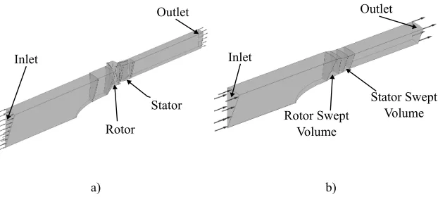
2-2 Computational domains of (a) the single passage bladed RANS
simu-lations and (b) the body force simulations. . . 14
2-3 Work coefficient vs. meridional distance through the rotor at: (a) 20%
span (b) 50% span (c) 80% span and (d) rotor trailing edge at 70%
corrected speed, andφ = 0.48. . . 15 2-4 Work coefficient vs. meridional distance through the rotor at: (a) 20%
span (b) 50% span (c) 80% span and (d) rotor trailing edge at 90%
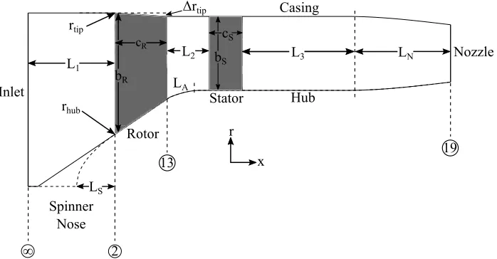
corrected speed, andφ = 0.48. . . 15 2-5 Meridional profile displaying the geometric parameters required for gas
path generation and station numbering. . . 18
2-6 Example of blade camber line. . . 23
2-7 Rotor chordwise work coefficient at 80% span comparison between a
blade with and without added incidence from the CFD simulations of
the example design shown later3. . . . . 24
2-8 Velocity triangle at the rotor trailing edge . . . 25
2-9 Camber lines for the example design shown later1 produced by running
2-10 Work coefficient vs. meridional distance through the Stage 67 rotor at:
(a) 20% span (b) 50% span (c) 80% span and (d) rotor trailing edge
for comparison of chordwise loading between a real machine and the
simplified stage for 90% corrected speed andφ = 0.48. . . 28 2-11 Computational domain created for internal flow simulations. . . 31
2-12 Work coefficient vs. meridional distance through the rotor at: (a) hub
(b) 50% span (c) tip and (d) rotor trailing edge at design corrected
speed andφ = 0.64. . . 34 2-13 Chordwise flow coefficient through the rotor at design corrected speed
and φ= 0.64. . . 35 2-14 Deviation through the rotor tip. . . 37
2-15 Work coefficient at rotor trailing edge during off-design (takeoff)
com-parison. . . 38
3-1 Comparison between NASA Stage 67 and simplified stage gas paths
and meridional blade profiles. . . 47
3-2 Work coefficient vs. meridional distance through the rotor at: (a) 20%
span (b) 50% span (c) 80% span and (d) rotor trailing edge at design
speed. . . 49
3-3 Mass flux along rotor trailing edge. . . 51
3-4 Computational domain for crosswind simulations. (a) Side view, (b)
front view, and (c) zoomed in view of nacelle and fan stage. . . 52
3-5 Nacelle casing used within full wheel simulations, where the dashed
line represent the casing extended axially downstream and the
dashed-dotted line is the rotation axis . . . 53
3-6 Separation size and FPR as a function of grid points used to show grid
3-7 Areas of separated flow within the nacelle at the (a) fully attached
condition, (b) separation point, and (c) highly separated condition. . 56
3-8 Mach number in plane tangent to crosswind velocity with (a) attached
flow and (b) highly separated flow. . . 57
3-9 Stagnation pressure ratio at rotor leading edge with (a) attached flow
and (b) highly separated flow. . . 58
3-10 Mass flux distribution at the fan face for the (a) fully attached
condi-tion and (b) highly separated condition. . . 59
3-11 Absolute flow angles at the fan leading edge for the (a) fully attached
condition and (b) highly separated condition. . . 61
3-12 Meridional velocity normalised by the blade rotation speed at 50%
span at the fan leading edge for the (a) fully attached condition and
(b) highly separated condition. . . 62
3-13 Change in incidence angles from design at the fan leading edge for the
(a) fully attached condition and (b) highly separated condition. . . . 62
List of Tables
2.1 Important characteristics of NASA Stage 67 rotor at 90% speed [11]. 12
2.2 Summary of the bladed simulations grid independence study performed
by Hill and Defoe (2018) [2]. . . 13
2.3 Summary of the body force grid independence study preformed by Hill and Defoe (2018) [2]. . . 13
2.4 Work coefficient RMS errors for NASA Stage 67 at 70% corrected speed and φ= 0.48. . . 16
2.5 Work coefficient RMS errors for NASA Stage 67 at 90% corrected speed and φ= 0.48. . . 16
2.6 Summary of the grid independence study for the example design in the next section. . . 32
2.7 Key design parameters. . . 33
3.1 Comparison of NASA Stage 67 and the simplified stage. . . 50
Nomenclature
Symbols
A Area
a Location of maximum camber
B Number of blades in a row
b Blade span
cBlade chord
cp Pressure coefficient
e Energy
F Thrust
f Force
h Enthalpy
i Incidence angle
K Compressibility correction factor
L Length
M Mach number ˙
m Mass flow rate ˆ
n Blade camber surface normal vectors
p Pressure
R Gas constant
s Spacing between blades
T Temperature
U Blade speed
U∗ Velocity ratio
~
V Velocity
~
W Relative velocity
α Absolute flow angle
β Relative flow angle
γ Specific heat ratio
δ Deviation
η Efficiency
κ Blade metal angle
ξ Change in blade angle
ρ Density
τ Shear stress
Υ Tip radius change parameter
φ Flow coefficient
ψpt Stagnation pressure rise coefficient
ψ Work coefficient
ω Angular velocity
Subscripts
13 Fan trailing edge quantity
19 Nozzle exit quantity
2 Fan face quantity
abs Absolute quantity
BF Body force quantity
BS Bladed simulation quantity
cCompressible
corr Corrected value
hubHub span location
i Incompressible
inletInlet boundary value
is Isentropic
LE Blade leading edge
m Meridional component
mid Mid span location
n Normal component
n% Location percent
R Rotor
ref Reference quantity
rel Relative quantity
S Stator
sliceSlice quantity
Spin Spinner nose
t Stagnation quantity
tip Tip span location
T E Blade trailing edge
x Axial component
y Crosswind quantity
δ Deviation
∞ Freestream quantity
Superscripts
A Area-averaged quantity
M Mass-averaged quantity
Abbreviations
BMA Blade Metal Angle
CFD Computational Fluid Dynamics
FPR Fan Stagnation Pressure Ratio
RANS Reynold-Averaged Navier-Stokes
Chapter 1
Introduction
In an effort to increase propulsive efficiencies in, and thereby reduce fuel
consump-tion from commercial aircraft, manufacturers are using lower fan stagnaconsump-tion pressure
ratios (FPR) and thus increasingly larger fan diameters in turbofan engines.
Early-generation geared turbofan engines with FPR of 1.4 and bypass ratios of 12 have
been shown to reduce fuel burn by up to 16% when compared to prior engines with
the same thrust range [1]. This reduction is expected to grow in the future as
de-creasing FPR are used [2]. This design trend requires ever-larger engine diameters,
which leads to increased weight; typically this increase is offset by reducing the length
of the nacelle casing. However, shorter nacelle inlets lead to an increased chance of
inlet distortion effects, which can negatively effect fan stage performance [3]. It is
critical for airframers to have the ability to assess the changes in external flow-fan
stage interaction caused by these changes in nacelle design.
To view this interaction, the airframer must be capable of modelling the fan stage.
It is an issue as typically the airframer would not have detailed fan stage geometry
because they are well protected by the engine manufacturer - this work serves to
resolve this problem. Through the use of 1D analysis to determine necessary stage
assumptions, a process is defined that generates a body force model intended for use
in assessing external flow-fan stage interaction.
1.1
Objective and High-Level Approach
The objective of this thesis is to present a process that allows for the creation of a
fan stage body force model without the need for a prior knowledge of detailed fan
geometry. The body force model generated is assessed on its ability to produce the
desired performance, capture trends that are found in real modern machines, and
reproduce the inlet distortion responses seen when detailed geometry is used. The
distortions of interest are those created by varying crosswind velocities. Crosswind
flow is defined as flow that moves perpendicular to the axis of rotation of the
turbo-machinery. The use of a body force fan model is critical for this process as it greatly
reduces computational costs, especially for inlet distortion cases. The reduction in
computational costs occurs because the body force replaces physical blade rows with
volumetric source terms. This replacement allows for the use of steady as opposed
to unsteady, computational fluid dynamics, and reduces the computational grid by
approximately two orders of magnitude.
1.2
Major Findings and Conclusions
In this thesis, two major topics are investigated. The first is the development of the
body force model design process and its ability to create a body force model that
produces the correct desired performance. The second topic is the effect of using
a model thus produced on inlet distortion response prediction compared to using a
detailed stage geometry.
Using the design process, a body force model representative of a high bypass ratio
spec-ified at design conditions. Design elements, such as desired chordwise and spanwise
loading distributions are examined. The chordwise loadings show excellent agreement
with the design intent at lower span fractions. The local root mean squared (RMS)
difference is approximately 4% of the maximum chordwise loading; however,
agree-ment decreases as span fraction increases, and this value increases to 15% in the outer
span. The spanwise loading distribution matches well with the design intent with a
local root mean squared difference of 0.6% .
The process is also used to create a body force model based on the performance
of an existing machine to determine the effects of the simplifications used to generate
the model. The overall performance at design is well matched with slight deviations
from the desired requirements, namely the FPR is 1.14% over the desired value. The
effect of simplification on the ability to capture distortion interaction effects on the
fan and nacelle performance was investigated. The simplification has little effect
on fan performance prediction. The maximum difference in the predicted incidence
angle during highly separated flow was 2.4◦ in the outer span, which is deemed as an
appropriate accuracy when considering the level of intended fidelity. The maximum
difference in predicted nacelle performance, measured using a metric which quantifies
the stagnation pressure loss in a 60◦ sector, occurred with highly separated flow; the
simplified stage over predicted the loss by 9%.
The intended use of this process is not to a produce a detailed, or realistic fan
stage design, but to produce a model that recreates the effect that a fan stage has on
the flow. It is a tool that is intended to be used during preliminary design of nacelles
1.3
Thesis Outline
This thesis is split into two major chapters, each responsible for one of the topics
mentioned. In Chapter 2, the body force formulation is described in detail and
its validation is demonstrated. The design process is detailed here along with the
implementation of this process into a commercial CFD framework. Finally an example
application of this process is demonstrated. In Chapter 3, this process is used to create
a body force model based on an existing stage as a design reference. The effects of
the simplifications employed are investigated, at both design condition and with inlet
distortion. Lastly, conclusions are drawn from this work and possible future plans are
1.4
Bibliography
[1] Game changing technology: Pratt & whitney geared turbofan engine reduces fuel
burn by 40 million gallons.
https://www.utc.com/en/news/2018/07/09/game-
changing-technology-pratt-whitney-geared-turbofan-engine-reduces-fuel-burn-by-40-million-gallon, 2018.
[2] B. Riegler and B. Bichlmaier. The geared turbofan technology opportunities,
challenges, and readiness status. 1st CEAS European Air and Space Conference,
September 2007.
[3] A. Peters, Z. S. Spakovszky, W. K. Lord, and B. Rose. Ultrashort nacelles for low
Chapter 2
Prediction of Crosswind
Separation Velocity for Fan and
Nacelle Systems Using Body Force
Models: Part 1: Fan Body Force
Model Generation Without
Detailed Stage Geometry
2.1
Introduction
In the design stage of an airframe, the external flow around all components must be
considered. This is certainly important around engine nacelles, where the external
flow will be affected by the operation of the fan. This interaction is dependent on
both the positioning of the fan stage within the nacelle and its operating condition
simplified model of the propulsion system. This is done to reduce computational costs
compared to traditional bladed Reynolds-averaged Navier-Stokes (RANS) methods.
These simplified models use steady computational fluid dynamics (CFD) simulations
for non-uniform inflow where normally unsteady simulations would be required, as
well as reducing the number of grid cells needed by approximately two orders of
magnitude within the turbomachinery blade rows [2].
These modeling approaches are discussed in detail in Godard et al. (2017) [3]. One
of the approaches commonly used in full airframe simulations involves using actuator
disks. Actuator disks work by imposing changes to flow direction and stagnation
quantities over a single plane but are limited in their ability to reproduce the effects of
the coupling between external flow and the fan. Godard et al. proposed that the main
reason for this inability comes from the fact that the actuator disk takes the inflow as
is and computes the outflow accordingly but lacks feedback effects [3]. Through-flow
or body force methods are another approach that is examined to help capture this
coupling effect however this is a higher fidelity approach and therefore requires more
information. Body force methods work by applying sources of momentum and energy
in the swept volumes where the blades would normally be, and were found to capture
the external flow-fan coupling more accurately than actuator disks [3].
Many variations of body force methods exist however they usually require the user
to have detailed blade geometry. Gong’s model [4] and its later refinements in Peters
et al. (2015) [1], Hill’s model [2] as well as a Lift-Drag model [5] are examples of these;
they require calibration based on experiments or more detailed computations which
include the blade rows in detail. This calibration therefore relies on detailed blade
geometry and entails additional computational cost. Models such as those proposed
by Hall et al. (2017) [6] and Pazireh and Defoe (2019) [7] have been shown to work
thickness information needed in Hall’s approach) and the gas path1 of the fan stage.
The modeling approach of Sato et al. (2019) [8] works without the need of fan blade
geometries but still requires information on the gas path, and blade leading and
trailing edge meridional2 profiles.
However, the airframer may not have selected what engines will be used, and even
if they have they may not be able to obtain the fan geometry and/or bypass duct gas
path from the engine manufacturer. This means that they would be unable to use the
body force methods mentioned above. Tools currently exist that allow for creation
of highly detailed stage and blade geometry, however they generally require more
experience with turbomachinery, as well as detailed information about the stage.
MULTALL is an open source turbomachinery design suite which takes basic stage
information and will generate 3D blades and gas paths [9]. Although simplified, these
inputs still require the user to have information on the blade performance which may
be unknown, such as blade rotation speed or stage work coefficient. The airframer
is not interested in the level of fidelity of the blades or the stage; all they require
is that the body force recreates the external-internal flow interaction. Therefore the
airframer desires to create this body force model based on information that they know
to some degree of accuracy, such as, the required thrust, limitations on engine size,
and estimation of the fan stagnation pressure ratio (FPR) at the design point.
The objective of this paper is to introduce and assess a body force model
gen-eration process which enables simulation of powered nacelles and/or full airframes
without any prior detailed fan geometry information. This process consists of 1D
analysis to determine the required change in flow quantities through the stage, as
well as generating simplified blade camber surfaces and a gas path. The full
MUL-TALL suite is not used since it requires too much input information, however certain
tools within the suite are utilized as will be described later. A number of assumptions
1Hub and casing radius as a function of axial position
and simplifications are used during these steps to determine the required information.
The key outcomes are that (1) the process enables creation of a body force model of
a fan stage without a priori knowledge of detailed fan geometry or gas path; (2) this
body force model, once implemented in a CFD framework, matches the design intent
performance at the design point; (3) this body force matches the desired spanwise
loading at the rotor trailing edge, which in this process is uniform, and provides a
reasonable estimate of the rotor chordwise loading similar to that found in modern
machines. With these outcomes met the resulting model can also be used to assess
off-design conditions.
In the first section of this paper the body force formulation is described in detail
and its validation is demonstrated. Next the design process is explained and the
selected camber shape is presented and validated. The implementation of this process
into a commercial CFD framework is discussed, and finally an example application
of this process is demonstrated.
2.2
Body Force Formulation
The concept of body force modeling involves replacing the physical rotor and stator
blades with momentum and energy sources. These sources are added across a
cir-cumferential region covering the radial and axial extent of the physical blades. These
sources are used to generate the flow turning, as well as the pressure and temperature
changes which occur in the real machine. These sources can be thought as a local
LE θ
x
Fn Fp
θ
x
TE LE TE
Fan Body force
Fan Body Force
Leading Edge
Trailing Edge x
θ
x
θ
Fn
Leading Edge
Trailing Edge Leading
Edge
Figure 2-1: Comparison of the physical blades (left) and to the source term model (right).
The momentum and energy equations are,
∂ρ~V
∂t +∇(ρ~V ~V
T) +∇p− ∇ ·τ =ρ~f (2.1)
∂ρet
∂t +∇(ρht ~
V)− ∇ ·(∇ ·τ) =ρ(~r×~ω)·~f (2.2)
where ρ is the fluid density, V~ is the flow velocity, p is the static pressure, et is stagnation energy (where ρht=ρet+p ), ht is stagnation enthalpy, r is radius,ω is angular rotation speed, and τ is the viscous stress. The equations are modified to account for the momentum and energy source terms, which are represented as a body
force per unit mass f.
The body force method chosen for this process is Hall’s model [6], because it
requires no calibration and therefore reduces the amount of stage information needed.
The source term per unit mass, here the incompressible normal force, fn,i, is defined
as:
fn,i=
2πδ 12W2/|n θ|
2πr/B (2.3)
The blade leading and trailing edge meridional profiles, and the full machine gas
path are also needed. The original Hall model was only intended to be used for
low speed machines (incompressible flow), so a correction factor is added to account
for compressibility since modern commercial engine fans operate at transonic relative
Mach numbers. This takes the form of an added compressibility correction,K, where:
fn,c =Kfn,i (2.4)
as used in Benichou et al. (2019) [10]. This correction uses the Prandtl-Glauert rule
in subsonic relative flow, and the Ackeret formula in supersonic relative flow,
K0 =
1
√
1−M2 M < 1
2
π√M2−1 M >1
(2.5)
and has an upper limit set to avoid instabilities as the relative Mach number
ap-proaches 1 giving,
K =
K0 K ≤3 3 K0 >3
(2.6)
Body force models exist that have added terms to account for the blockage effects
caused by the blades; this can be seen in the model used in Benichou et al. (2019)
[10]. Including blockage adds complexity as it requires information on blade thickness.
This was neglected in the current approach as the aim is not to generate full blade
shapes, and as will be shown later is not required to accurately predict the loading in
however the upstream influence of a fan on incoming flow is not significantly impacted
by the viscous losses in blade rows [6] and are therefore neglected in the body force
model used in this paper.
2.3
Assessment of Body Force Approach
A single passage bladed RANS simulation is compared against a body force model
to assess the approach both with and without the compressibility correction at the
design flow coefficient,
φ= Vx
Umid
(2.7)
of 0.48, whereUmid is the rotor blade speed at mid-span. The machine used is NASA Stage 67 [11]. The important features of this machine are shown in Table 2.1. The
overall, spanwise, and chordwise loading is examined for both the 70% and 90%
speedlines.
Table 2.1: Important characteristics of NASA Stage 67 rotor at 90% speed [11].
Parameter Value Parameter Value
ωcorr(rad/s) 1512 B 22
Mrel,tip 1.2 Vx
M
Umid 0.5
FPR 1.48 rhub rtip
inlet
0.375
˙
mcorr (kg/s) 31.1
rhub rtip
outlet 0.478
True Chord Aspect Ratio 1.56
The simulations were run using Ansys CFX 16 [12]. The grids and computational
approach are the same as those used in Hill and Defoe (2018) [2]. The bladed Stage
67 simulation uses a single passage containing 3.58×10⁶ cells. Two grids were used to
than 1% change is seen between the stagnation pressure ratio and isentropic efficiency
and it was therefore determined that the medium grid is sufficient. The simulations
are steady state, and use the shear-stress-transport turbulence model. The stagnation
quantities are set at the inlet and a mass flow rate boundary condition is used at the
outlet. In this paper, blades with zero shear stress surfaces were used so that a direct
comparison could be made against the body force model which includes only the
turning (normal) force in the blade rows. The body force model consisted of a 1/16
annulus slice containing 279,760 cells. In Table 2.3 a summary of the body force
grid independence study is shown. The boundary conditions are the same as in the
bladed simulations. The computational domains are shown in Figure 2-2. Further
information on the computational setup can be found in Hill and Defoe (2018) [2].
Table 2.2: Summary of the bladed simulations grid independence study performed by Hill and Defoe (2018) [2].
Medium Grid Fine Grid Percent Change
Rotor Cell Count 1.78x10⁶ 2.45x10⁶ 37.6
FPR-1 0.493 0.496 0.71
Rotor ηis 92.3% 92.3% 0
Table 2.3: Summary of the body force grid independence study preformed by Hill and Defoe (2018) [2].
Medium Grid Fine Grid Percent Change
Cell Count 279,760 609,500 117%
Inlet
Rotor
Stator Outlet
a) b)
Inlet
Outlet
Rotor Swept Volume
Stator Swept Volume
Figure 2-2: Computational domains of (a) the single passage bladed RANS simula-tions and (b) the body force simulations.
The work coefficient, defined as
ψ = ht−ht,inlet
Umid2
(2.8)
as a function of chord is shown in Figures 2-3 and 2-4 for 70% and 90% corrected
speed,
%ωcorr =
ω
q Tt Tt,ref
,
ωdes q
Tt Tt,ref
(2.9)
respectively. The figures include results from the Hall body force model with and
without the compressibility correction as well as the single-passage results, which are
% Chord
0 20 40 60 80 100
ψ -0.1 0 0.1 0.2 0.3 % Chord
0 20 40 60 80 100
-0.1 0 0.1 0.2 0.3 % Chord
0 20 40 60 80 100
0.1 0.2 0.3
0.1 0.2 0.3 0.4
% Span 0 20 40 60 80 100 Single Passage Bladed
a) b) c) d) 0 -0.1 Fn,i Fn,c ψ ψ ψ
Figure 2-3: Work coefficient vs. meridional distance through the rotor at: (a) 20% span (b) 50% span (c) 80% span and (d) rotor trailing edge at 70% corrected speed, and φ = 0.48.
% Chord
0 20 40 60 80 100
Work Coefficient -0.1 0 0.1 0.2 0.3 % Chord
0 20 40 60 80 100
Work Coefficient -0.1 0 0.1 0.2 0.3
Single Passage Bladed Body ForceWithout K Body ForceWith K
% Chord
000 20 40 60 80 100
W or k C oe ff ic ei nt -0.1 0 0.1 0.2
0.3 20% Span
% Chord
0 20 40 60 80 100
Work Coe fficie nt -0.1 0 0.1 0.2
0.3 50% Span
% Chord
0 20 40 60 80 100
Work Coe fficie nt 0 0.1 0.2 0.3
0.4 80% Span
Work Coefficient
0.1 0.2 0.3 0.4
% Span 0 20 40 60 80
100 TE Spanwise Profiles Single Passage/Bladed
KFn KFn
% Chord
0 20 40 60 80 100
Work Coe fficei nt -0.1 0 0.1 0.2
0.3 20% Span
% Chord
0 20 40 60 80 100
W or k C oe ff ic ie nt -0.1 0 0.1 0.2
0.3 50% Span
% Chord
0 20 40 60 80 100
Work Coe fficie nt 0 0.1 0.2 0.3
0.4 80% Span
Work Coefficient
0.1 0.2 0.3 0.4
% Span 0 20 40 60 80
100 TE Spanwise Profiles Single Passage/Bladed
KFn KFn
% Chord
0 20 40 60 80 100
Work Coe fficei nt -0.1 0 0.1 0.2
0.3 20% Span
% Chord
0 20 40 60 80 100
Work Coe fficie nt -0.1 0 0.1 0.2
0.3 50% Span
% Chord
0 20 40 60 80 100
Work Coe fficie nt 0 0.1 0.2 0.3
0.4 80% Span
Work Coefficient
0.1 0.2 0.3 0.4
% Span 0 20 40 60 80
100 TE Spanwise Profiles Single Passage/Bladed
KFn KFn
% Chord
0 20 40 60 80 100 -0.1
0 0.1 0.2
0.3 20% Span
% Chord
0 20 40 60 80 100
Work Coe fficie nt -0.1 0 0.1 0.2
0.3 50% Span
% Chord
0 20 40 60 80 100
Work Coe fficie nt 0 0.1 0.2 0.3
0.4 80% Span
Work Coefficient
0.1 0.2 0.3 0.4
% Span 0 20 40 60 80
100 TE Spanwise Profiles Single Passage/Bladed
KFn KFn
Single Passage Bladed
Fn,i Fn,c 0 a) b) c) d) ψ ψ ψ ψ
The root mean squared (RMS) difference in local chordwise and spanwise work
coefficient as a percent of total change in bladed simulation work coefficient along the
chord (mass averaged in the spanwise case) between the body force (BF) models and
the bladed simulations (BS), defined as
%RM S = s
Rc
0(ψBS−ψBF) 2 dx
c
(ψBS,T E −ψBS,LE)×100 (2.10)
is shown in Tables 2.4 and 2.5.
Table 2.4: Work coefficient RMS errors for NASA Stage 67 at 70% corrected speed and φ = 0.48.
fn,i %RMS fn,c %RMS Improvement
20% Span 7.78% 6.62% 1.16%
50% Span 7.27% 2.74% 4.53%
80% Span 7.98% 3.75% 4.23%
Spanwise 4.50% 4.30% 0.20%
Table 2.5: Work coefficient RMS errors for NASA Stage 67 at 90% corrected speed and φ = 0.48.
fn,i %RMS fn,c %RMS Improvement
Difference Difference
20% Span 9.25% 5.37% 3.88%
50% Span 10.9% 1.81% 9.09%
80% Span 12.7% 2.15% 10.5%
Spanwise 8.34% 3.42% 4.92%
overall and chordwise loadings. The correction factor has a greater influence the
larger the relative Mach number becomes; this is seen as the span fraction increases
and as the corrected rotational speed is increased. In the 70% corrected speed case
the improvement increases by approximately 3% as the span fraction increases, and
in the 90% corrected speed case this increases even further to approximately 6%.
The reason for this larger improvement in the 90% corrected speed case is due to
the fact that the relative Mach numbers are increased throughout the rotor. This
is also seen in the fact that the improvement more than doubles throughout in this
higher corrected speed case. The results show that the body force model with a
compressibility correction is capable of matching the loadings to within 7% which is
deemed as an acceptable level of accuracy for this design process.
2.4
Fan Stage Design Approach
We take the fan design point to be cruise, as this is the typical design condition
for low fan pressure ratio commercial aircraft engines [13] which are of increasing
interest in modern design. The benefit of selecting this typical design condition is
that this is usually where the designer will have the most information about required
performance. This condition requires the specification of a cruise altitude and flight
Mach number. These are quantities an airframer would normally know and provide
the information needed to find inlet stagnation quantities. We employ 1D analysis to
determine the flow properties through the stage to meet the desired performance at
cruise; based on the resulting flow properties as well as a series of assumptions and
geometric constraints, the gas path can be defined.
The fan pressure ratio and net thrust are required inputs. The input geometric
axial distances upstream of, between, and downstream of the blade rows (L1/cR,
L2/cR, L3/cR), nozzle contraction length (LN/cR), hub curvature length (LA/cR) and fractional tip radius change through the rotor (∆rtip/rtip). A diffusion factor is specified to determine the number of rotor and stator blades, or these can be directly
specified. If an elliptical spinner nose is desired, the axial length of the spinner nose,
LSpin, is also needed, and is specified as a percent of a linear spinner nose length. The body force model is created to generate a set fan stagnation-to-stagnation pressure
ratio at a corrected mass flow which, combined with the gas path geometry, achieves
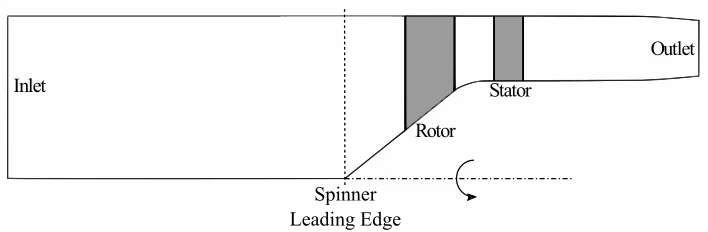
the desired thrust. Figure 2-5 shows the generic meridional profile of the gas path
and illustrates the definitions of the geometric parameters.
Inlet
Nozzle
Rotor
Stator Hub
Casing
Spinner Nose
rhub
rtip
L1
bR
cR L
2
LS
L3 LN
cS
bS
x r Δrtip
∞ 2
13 19
LA
Figure 2-5: Meridional profile displaying the geometric parameters required for gas path generation and station numbering.
The assumptions made are:
1. the axial velocities at the leading and trailing edge of the blade rows are equal
and constant along the span,
2. the bypass ratio is high enough that the core flow contribution to thrust
gener-ation and the core suction effect on flow in the fan rotor is negligible,
4. the flow is in the meridional direction at fan inlet.
From assumption (2), we do not include a bifurcation into a core duct in the gas path.
A simple linear scaling is used to set the blade tip relative Mach number. From
literature it was found that modern day fans with pressure ratios of 1.6 would be
expected to have a tip relative Mach number of approximately 1.4 [13, 14]. We apply
this scaling to set our tip relative Mach number based on the design fan pressure ratio
(F P R):
Mrel,tip = 1.4
1.6F P R (2.11)
At design, hub and casing boundary layers are thin and fully attached due to the
high Reynolds numbers in practical engine fans and thus we assume no changes in
stagnation quantities up to the fan face; these are then set by the flight condition.
2.4.1
Stage Performance and Gas Path
Application of control volume analysis to the flow going through the engine yields the
standard expression for the thrust
F = ˙m(V19−V∞) +A19(p19−p∞) (2.12)
where F is thrust, ˙m is the mass flow rate, and A is passage area. The thrust, flight velocity, and freestream static pressure are known at the outset, with the other
quantities to be determined; this is done using a quasi-1D approach. Two cases can
exist, depending on whether the exhaust nozzle is choked or not. The nozzle is choked
if
F P Rpt,∞ p∞
for air with specific heat ratio γ = 1.4. If the nozzle is choked the nozzle exit static pressure is
p19 =p∞
F P R
1.893
1 +
γ−1 2
M∞2
γγ−1
(2.14)
If the nozzle is not choked the nozzle exit static pressure is equal to the atmospheric
static pressure:
p19=p∞ (2.15)
The nozzle velocity, assuming isentropic flow, is
V19=M19 "
γR F P R
γ−1 γ T
∞ 1 + γ−21
M∞2
1 + γ−21
M192
!#0.5
(2.16)
If the nozzle is choked then M19 = 1 and if it is unchoked it is determined by
M19=
pt,∞F P R
p∞
γ−γ1 −1 γ−1
2 0.5 (2.17)
If the flow is choked, the mass flow and nozzle area are then given by the simultaneous
solution of Equations 2.12 and the corrected flow per unit area equation applied at
station 19,
˙
m= Ap19pt,19
Tt,19 r
γ RM19
1 + γ−1 2 M19
2
−2(γγ+1−1)
. (2.18)
In 2.18, the stagnation quantities are the mass-weighted averaged values. To keep
the body force model as simple as possible, we design for uniform spanwise work input
so that the local values are everywhere equal to the mass-weighted averages.
If the flow is unchoked, the mass flow rate is directly calculated from Equation
2.18 to determine the nozzle exit area.
The axial Mach number at the fan face (station 2) is found from Equation 2.18
given the fan inlet area (computed from the tip radius and hub-to-tip ratio) and the
now-known mass flow rate. This Mach number is then used to determine the static
temperature at the fan face.
The assumption of equal leading and trailing edge axial velocities along with the
choice of F P R allows the rotor trailing edge area to be calculated. In doing so we neglect the effect of swirl on the required rotor exit area, however, within the design
space typically of interest, swirl angles will normally be well under 30◦ and there is
only a minor effect on the passage area [15].
The gas path shape through the rotor is generated using straight line hub and
casing curves. This means that the axial velocity will vary within the blade row, but
greatly simplifies the generation of the gas path. A parameter, Υ, which is a fraction
of the fan leading edge span sets the amount of tip radius change through the rotor,
∆rtip = Υ(rcas,LE−rhub,LE) (2.19)
Downstream of the rotor the casing radius is constant.
The slope of the hub through the rotor is set to meet the required decrease in
passage area while keeping the leading and trailing edge axial velocities equal.
Downstream of the rotor trailing edge, the hub radius curves back towards axial
over some desired fraction of the distance between rotor and stator (LA). The stator span is set to be constant along the chord. In reality the removal of swirl would require
a decrease in passage area, but by the same logic applied to the determination of the
rotor trailing edge area, this effect is normally small.
The spinner length determines its shape. If the axial length is less than that of a
straight line with the rotor hub slope extended to zero radius, then the spinner nose
extends to zero radius upstream with the tangent to the ellipse at the nose purely
radial. Otherwise, a conical spinner is used with the rotor hub line extended directly
down to zero radius.
2.4.2
Blade Performance and Camber
The rotor inlet velocity triangle at the tip, which is determined by the axial Mach
found using Equation 2.18 and the relative Mach number found using Equation 2.11
determines the rotation speed of the rotor blades.
A camber surface is needed for the body force model. Camber lines are determined
at set span fractions; in the current approach hub, mid, and tip span fractions are
used. The camber surface is generated by fitting a 3D surface which passes through
these lines.
Chordwise loading distribution has been shown to have an effect on inlet
distor-tions [6], therefore one of the aims is to generate a body force model with a camber
surface that produces realistic chordwise loading distributions, while remaining
rela-tively simple. The solution employed is to use camber shapes defined by a combination
of a circular arc and a straight line. An example of this camber shape is shown in
Figure 2-6. In physical blades the highest loading tends to be in the leading edge
region, however in the Hall body force model (Equation 2.3) the loading scales with
deviation, which tends to increase towards the trailing edge at design. The intent of
pushing all camber curvature forward is to combat this effect. The straight line in
the rear section of the chord works to ensure that the required overall flow turning is
met as the Hall model acts to reduce the deviation. A range of circular-straight line
dividing locations were tested, and it was found that a 50/50 split between circular
arc and straight line provides the best combination of guaranteeing the correct flow
turning and chordwise loading distribution accuracy as shown later. It should be
increases the accuracy of the loading distribution of the body force model. This is
a significant difference compared to the no blade information process used by Sato,
Spotts, and Gao (2019) [8] as no real attempt was made to capture realistic chordwise
loading in that paper.
0 50
% Chord
r
θ
0 50 100
Circular Arc Straight Line
Figure 2-6: Example of blade camber line.
In the design velocity triangles the meridional velocity is used as opposed to the
axial velocity. This is important because of the significant radial velocities in the
rotor, especially near the hub. The consequence is that the velocity triangles and
hence camber angles are dependent on the streamsurface inclination since the leading
and trailing edge axial velocities are assumed constant.
At the rotor leading edge a small positive incidence of 2◦ is used; this along with
the design velocity triangles sets the rotor inlet camber angle. The incidence is added
to provide a more realistic chordwise loading. It increases the blade loading and flow
deflection in the rotor leading edge region. This also helps ensure that the chordwise
loading distributions match predicted trends when the assumption of constant axial
velocity is not realized when employing the model within a CFD simulation; if the
axial velocity exceeds the assumed value it will cause negative incidence at the leading
edge which can result in local work removal. The positive incidence acts to counteract
without the added incidence from the example design described later3 to demonstrate
the difference in work addition. In the blade with 0◦ incidence the stagnation enthalpy
in the first 20% chord drops below the freestream stagnation enthalpy; this could alter
the expected distortion interaction behaviour. Adding the incidence eliminates this
decrease in the leading edge region. The stator leading edge camber angle is set by
assuming zero incidence. Zero incidence was used for the stator leading edge because
there is no change in work across the stator which eliminates the need to add incidence
to improve the chordwise loading distribution.
% Chord
0 20 40 60 80 100
Work Coefficient
-0.1 0 0.1 0.2 0.3 0.4
0.5 Rotor Chordwise Work at 80% Span
Camber with 2 deg incidence Camber with 0 deg incidence
Figure 2-7: Rotor chordwise work coefficient at 80% span comparison between a blade with and without added incidence from the CFD simulations of the example design shown later3.
The rotor trailing edge flow angles are set based on the required work input, using
the Euler turbine equation,
cp(Tt,T E−Tt,LE) = ω(rT EVθ,T E −rLEVθ,LE), (2.20)
the design choice to have a constant spanwise work input/pressure rise, and flow
deviation. The stator trailing edge is set to remove the swirl from the flow. The
trailing edge angles in both blade rows account for deviation. Trailing edge deviation
is estimated using a modified form of Carter’s rule [13]:
δT E = 0.23
2a c
2
+ α 500
!
ξs c
0.5
(degrees). (2.21)
where the maximum camber of the blade is at an axial distance a from the leading edge, c is the axial chord length, α is the exit flow angle (β in the rotor), ξ is the overall change in blade angle, and s is the pitch (spacing between blades). Carter’s rule is intended for fully circular blade camber shapes; a modification is made toato account for the adjustment of the location of maximum camber from the mid point to
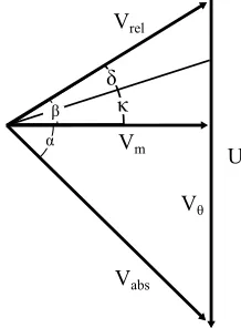
the new value of 37.5% chord (a= 0.375). The relationship between the flow angles (α and β), blade angle (κ), and deviation (δ) at a rotor trailing edge are illustrated using the generic velocity triangle shown in Figure 2-8.
U
Vθ
Vrel
Vabs
κ δ
β
Vm α
Figure 2-8: Velocity triangle at the rotor trailing edge
The 2D camber line sections are stacked using the open-source turbomachinery
design suite MULTALL’s geometry and grid generator Stagen. The information
re-quired for Stagen is the camber distribution and the corresponding axial and radial
coordinates through the gas path at the set span fractions (0% and 100% are required,
however additional span fractions can be supplied to further constrain the design) and
grid based on the information given; the number of spanwise sections generated is
equal to the number of radial grid points requested. The current maximum of 64
points is used here, which has been shown to be an adequate number of radial grid
points in body force models [2]. The thickness distribution is set within Stagen to
produce blades of negligible thickness such that the maximum thickness is less than
1% of the blade chord. Blade thickness information is not required for the body force
model, and therefore this is done so the camber surface extraction provides a good
estimate. The blade sections are stacked with their centroids lying along a radial line
through the centroid of the hub blade section. Shown in Figure 2-9 are the camber
lines that are produced by Stagen. The grid points on the blade surfaces are then
ex-tracted and this is used to generate the 3D blade shapes. The camber surface is found
by extracting the average of the rθ coordinates of the pressure and suction sides of the 3D blade shapes at each axial location. Finally the camber surface normal vectors
used in the compressibility-corrected Hall body force model are calculated using the
MATLAB [16] built in function “surfnorm”. For more information on how Stagen
works refer to Denton (2017) [9].
0 50
r
θ
% Chord
0 50 100
0.45 0.5 0.55 0.6 0.65 0.7 0.75
0.9 1 1.1 1.2 1.3 1.4 1.5
Hub Tip 50% Span
25% Span
75% Span
Figure 2-9: Camber lines for the example design shown later4 produced by running Stagen. Hub, 50% Span, and Tip camber lines are supplied to Stagen
2.5
Assessment of Camber Distribution
The simplified camber shape is assessed by using NASA Stage 67’s gas path and
overall performance specifications atφ= 0.48 and 90% corrected speed. The purpose is to determine how accurately a half circular arc, half straight line camber distribution
can reproduce the real stage’s chordwise loading. Leading and trailing edge meridional
profiles, as well as the gas path are kept the same as the existing NASA Stage 67 to
isolate loading changes caused by camber shape. The trailing edge blade angles for
the simplified camber distribution are iteratively adjusted to minimize the spanwise
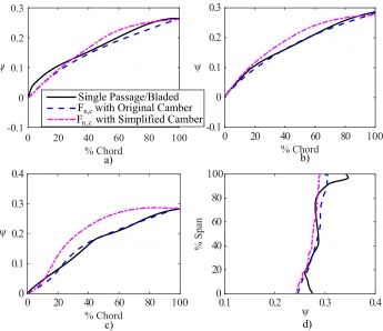
work coefficient distribution %RM S value at the trailing edge between the simplified and the original camber. The loading distributions are shown in Figure 2-10. The
spanwise loading (shown in Figure 2-10 (d)) %RM S difference value is 3.19%; with the outer region having a larger contribution to this difference. The work coefficient
in the outer region has a higher sensitivity to adjustments in blade angle which
leads to increased computational costs to reduce the %RM S difference in this region, therefore the accuracy of the trailing edge blade angle was iterated to ±0.05◦. The chordwise loadings display similar overall trends especially at lower span fractions
with the %RM S difference being 6.48% and 7.43% along the 20% and 50% span lines respectively. This slight difference is due to the modified distribution having larger
work addition within the first 50% chord, but this is expected as this is where blade
turning occurs. As span fraction increases this difference becomes more evident as the
%RM S difference increases to 13.2%; again this stems from the increased sensitivity due to blade angles changes in the outer span region. The %RM S difference provides a way to quantitatively compare the loading distributions to those of a real machine
however it is expected that the loadings distributions will not be exactly the same, as
the camber distributions are different. The general trends in the rate of work addition
% Chord
0 20 40 60 80 100
-0.1 0 0.1 0.2 0.3 % Chord
0 20 40 60 80 100
-0.1 0 0.1 0.2 0.3 % Chord
0 20 40 60 80 100
0 0.1 0.2 0.3 0.4
0.1 0.2 0.3 0.4
% Span 0 20 40 60 80 100 Single Passage/Bladed
Fn ,c with Simplified Camber Fn,c with Original Camber
ψ ψ ψ ψ a) b) d) c)
Figure 2-10: Work coefficient vs. meridional distance through the Stage 67 rotor at: (a) 20% span (b) 50% span (c) 80% span and (d) rotor trailing edge for comparison of chordwise loading between a real machine and the simplified stage for 90% corrected speed and φ= 0.48.
2.6
Estimating Operating Conditions for Off-Design
Thrust and Mass Flow
One of the intended uses of the models produced by the design process is to allow
airframers to investigate external-fan interactions at a variety of different conditions.
To investigate off-design conditions the user must know the fraction of design inlet
corrected mass flow,
˙
as well as the flight and atmospheric conditions. If the off-design operating point
yields an unchoked nozzle, inlet corrected mass flow is a function of the fan pressure
ratio and thus rotational speed. When investigating the off-design conditions it is
assumed that the fan is operating along the working line; in CFD this requires the
outlet boundary condition to be set at a constant pressure. The fact that, in general,
the flow coefficient is nearly a constant along a fan’s working line is used to assume
a linear relationship between the fraction of design inlet corrected mass flow and the
fraction of design corrected speed
˙
mcorr ˙
mcorr,des
= ωcorr
ωcorr,des
(2.23)
This yields an initial guess for the rotational speed required to drive a certain mass
flow through the machine.
With the mass flow supplied the fan inlet axial Mach number can be found using
Equation 2.18 at the fan face and subsequently the static temperature can be found.
With the axial Mach number and static temperature, the axial velocity is known.
It is again assumed that the axial velocity is equal at the rotor leading and trailing
edges. While this assumption is acceptable for the design condition it will be far less
accurate off-design, however this is only used as an initial estimate which is then later
corrected through an iterative process. Using the new velocity triangles and the blade
angles set at design the Euler turbine equation, Equation 2.20, is used to determine
the rotor outlet stagnation temperature, and this is then used to determine the rotor
outlet stagnation pressure. The stagnation quantities are found at the hub, 50%
span, and the casing; a parabolic curve is then fit to these points and that is used to
analytically mass average the rotor outlet stagnation conditions. Using the stagnation
quantities at the rotor outlet the same steps as before are used to determine the axial
velocity, static temperature, and static pressure at the nozzle exit. With the static
for the mass flow rate to be computed. This mass flow rate is compared to the desired
mass flow rate and the process is repeated with the rotational speed altered until the
desired mass flow rate is achieved. This provides an initial guess for the rotational
speed, however CFD simulations must be run and the rotational speed adjusted to
verify that the off-design operating point has been correctly found. An example of
this process is shown later in this paper and the off-design predictions are compared
to those found using CFD and the overall 1D performance prediction is matched to
within 2%.
2.7
Implementation of the Body Force Model
Gen-eration Approach
The design process has been implemented as a MATLAB [16] code, but could be
im-plemented in any scientific computing system. It generates the hub and casing curves
as well as the 2D blade camber lines at the hub, 50%, and tip span fractions. The
blade camber surface extraction process is also done within MATLAB. The process
runs on a personal workstation and is computationally inexpensive. Computational
run times for all steps (including Stagen) are typically under two minutes.
2.8
Implementation in 3D CFD
Hub and casing curves, as well as the the blade leading and trailing edge profiles are
imported into grid generation software (here, Pointwise v18 [17]) to generate the gas
path and demarcate blade swept volumes, which must be designated as separate cell
zones.
Shown in Figure 2-11 is a computational domain created using this process. The
rotor leading edge respectively. These are set far enough away to provide clean inflow
and avoid possible interactions with the blade rows. The process creates a constant
radius (equal to blade tip radius) casing curve upstream of the rotor blades. It should
also be noted that in the design point simulation the outlet nozzle is manually cut
slightly before the throat area(A∗); in the example case this was at A/A∗ of 1.08 (nozzle length cut by %10 before the throat area). This was done to avoid having a
Mach number equal to one occurring at a boundary condition, which was found to
lead to stability issues in some solvers.
Inlet
Rotor
Stator
Outlet
Spinner Leading Edge
Figure 2-11: Computational domain created for internal flow simulations.
Four grid levels are used to assess grid independence. A 5-degree slice of the full
machine is used with uniform inflow. This saves computational cost as the body force
model produces circumferentially uniform flow when the inflow is uniform.
Simula-tions are run at the design operating point for the design detailed in the next section.
All grids are fully structured using hexahedral cells with higher mesh density in the
bladed areas. A summary of the grids tested is in Table 2.6. Only a 0.9% change
in pressure rise coefficient was seen from the second finest grid to the finest grid and
Table 2.6: Summary of the grid independence study for the example design in the next section.
Overall Cell Count (x,r,θ) Grid Count Percent Change in Pressure Rise Coefficient
30024 (147,25,10) N/A
123480 (288,50,10) 8.1%
464310 (474,100,11) 1.5%
914860 (621,150,11) 0.9%
The computations are carried out using Ansys CFX v18.2 [12], using the same
boundary condition types described in the NASA Stage 67 body force simulations at
the design operating point, however at off-design operating points the outlet static
pressure is fixed based on the atmospheric conditions being tested and the rotational
speed is adjusted until the desired mass flow is reached. This is done to remain on
the fan working line. The hub and casing are set as zero shear stress walls as the
model assumes no losses.
2.9
Example Application of Process
In this section we present an example application of the model generation process
and its implementation into CFD. The main purpose of this example is to show the
level of expected accuracy of the desired performance at design and therefore assumes
that there is no inlet distortion or separation. In part 2 of this paper5 the ability to
predict these flow phenomena is examined. The example design discussed is based a
on high-bypass ratio turbofan engine for a medium-range jet airliner. The geometric
values, as well as the desired thrust are based on publicly available information found
on the Pratt & Whitney 1500G engine [18]. The key design parameters that are used
in this example are shown in Table 2.7.
Table 2.7: Key design parameters.
Parameter Value Parameter Value
FPR 1.4 bR/cR 2.33 Thrust at cruise 16.75kN bS/cS 2.25 Fan tip diameter 1.85m L1 8 Fan hub-to-hip ratio 0.3 L2 0.813 Cruise Mach number 0.78 L3 2
Cruise altitude 10668m LN 2
In this example application the number of rotor and stator blades is supplied
based on the Pratt & Whitney 1500G engine, and are 18 and 36 respectively. The
spinner nose is set such that the rotor hub slope line is extended to zero radius.
2.9.1
Results at Design Point
These inputs produce a stage with the gas path shown in Figure 2-11. The rotational
speed of the rotor (camber lines shown in Figure 2-9) is 374 rad/s and the required mass flow computed is 182 kg/s. The computed increase in the mass averaged fan stagnation pressure ratio across the rotor (FPR-1) was found to be 0.395 which is
1.25% below the design intent and the mass averaged stage work coefficient was found
to be 1.9% lower than the desired value. Using the mass averaged Mach number at the
outlet boundary it was found that the area which would create choked flow was 0.8%
lower than that generated by the design code. This resulting smaller area required
is a result of the stage slightly under predicting the FPR and work coefficient. If
and trailing edge spanwise work coefficients are shown. The spanwise trailing edge
work distribution has an RMS difference of 0.6% from the mass averaged overall work
coefficient, so the goal of uniform outlet stagnation temperature is largely achieved.
% Chord
0 20 40 60 80 100
-0.1 0 0.1 0.2 0.3 0.4 0.5 % Chord
0 20 40 60 80 100
-0.1 0 0.1 0.2 0.3 0.4 0.5 % Chord
0 20 40 60 80 100
-0.1 0 0.1 0.2 0.3 0.4 0.5 % Chord 0.5 0.55 0.6 0.65 0.7
Work Coefficient -0.1 0 0.1 0.2 0.3 0.4 0.5 Hub % Chord 0.5 0.55 0.6 0.65 0.7
Work Coefficient -0.1 0 0.1 0.2 0.3 0.4
0.5 50% Span
% Chord 0.5 0.55 0.6 0.65 0.7
Work Coefficient -0.1 0 0.1 0.2 0.3 0.4 0.5 Casing KFn TLAB Prediction Work Coefficient
0.3 0.35 0.4 0.45 0.5
% Span 0 20 40 60 80
100 TE Spanwise Profile Fn,c 1D Prediction ψ ψ ψ % Span ψ a) b) d) c)
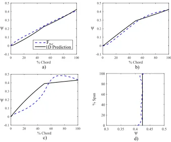
Figure 2-12: Work coefficient vs. meridional distance through the rotor at: (a) hub (b) 50% span (c) tip and (d) rotor trailing edge at design corrected speed and
φ= 0.64.
The loading is compared against a 1D prediction generated using the Euler turbine
equation and assuming constant axial velocity through the blade, as well as a linear
build-up of in deviation along the chord. The 1D prediction has a discontinuity
of slope at the transition from circular arc to straight line camber. The chordwise
loading is well predicted at lower span fractions with % RMS difference between
the 1D prediction and the CFD being 4.12% and 4.09% at the 20% and 50% span
fractions respectively, however as span fraction increases to 80% span the accuracy
![Table 2.2: Summary of the bladed simulations grid independence study performedby Hill and Defoe (2018) [2].](https://thumb-us.123doks.com/thumbv2/123dok_us/1341644.1167074/32.612.152.498.575.642/table-summary-bladed-simulations-independence-study-performedby-defoe.webp)