University of Windsor University of Windsor
Scholarship at UWindsor
Scholarship at UWindsor
Electronic Theses and Dissertations Theses, Dissertations, and Major Papers
2018
Machine Learning Approaches for Cancer Analysis
Machine Learning Approaches for Cancer Analysis
Alkhateeb Abedalrhman University of Windsor
Follow this and additional works at: https://scholar.uwindsor.ca/etd
Part of the Computer Sciences Commons
Recommended Citation Recommended Citation
Abedalrhman, Alkhateeb, "Machine Learning Approaches for Cancer Analysis" (2018). Electronic Theses and Dissertations. 7597.
https://scholar.uwindsor.ca/etd/7597
This online database contains the full-text of PhD dissertations and Masters’ theses of University of Windsor students from 1954 forward. These documents are made available for personal study and research purposes only, in accordance with the Canadian Copyright Act and the Creative Commons license—CC BY-NC-ND (Attribution, Non-Commercial, No Derivative Works). Under this license, works must always be attributed to the copyright holder (original author), cannot be used for any commercial purposes, and may not be altered. Any other use would require the permission of the copyright holder. Students may inquire about withdrawing their dissertation and/or thesis from this database. For additional inquiries, please contact the repository administrator via email
MACHINE LEARNING APPROACHES FOR CANCER ANALYSIS
by
Abedalrhman Adnan A. Alkhateeb
Windsor, Ontario, Canada
© 2018 Abedalrhman Alkhateeb A Dissertation
Submitted to the Faculty of Graduate Studies through the School of Computer
Science in Partial Fulfillment of the Requirements for the Degree of Doctor of
July 12, 2018
Machine Learning Approaches for Cancer Analysis
by
Abedalrhman Alkhateeb
APPROVED BY:
_____________________________ D. Zhu, External Examiner
Wayne State University
_____________________________ L. Porter
Department of Biological Sciences
_____________________________ A. Ngom
School of Computer Science
_____________________________ J. Lu
School of Computer Science
_____________________________ L. Rueda, Advisor
Declaration of Co-authorship /
Previous Publication
I. Co-Authorship
I hereby declare that this thesis incorporates material that is result of joint research, as follows:
Chapter 2 of the thesis was co-authored with L. Rueda. We both contributed in finalizing the idea
and follow-up discussions, A. Alkhateeb has implemented the method, experimental design, and the data
analysis. A. Alkhateeb and L. Rueda both contributed in writing the contents of the chapter.
Chapter 3 of this paper was co-authored with S. Singireddy, I. Rezaeian, and L. Rueda. L. Rueda is
the one who suggested the idea, and then A. Alkhateeb and L. Rueda participated in discussing how to
model the time series problem. S. Singireddy participated in pre-processing the dataset, A. Alkhateeb has
implemented the methods. A. Alkhateeb, I. Rezaeian, and L. Rueda have participated in writing the text
of paper.
Chapter 4 was co-authored by R.Etemadi, AA. Tabl, N.Mangalakumar, H. Pham, W. ElMaraghy, L.
Rueda, and A. Ngom.
In [R. Etemadi, A. Alkhateeb, I. Rezaeian, and L. Rueda ”Identification of discriminative genes for
pre-dicting breast cancer subtypes,” IEEE International Conference on Bioinformatics and Biomedicine (BIBM)
2016 Dec 1 (pp. 1184-1188). IEEE.] R. Etemadi and L. Rueda have discussed the initial idea, R. Etemadi
has implemented the methods. A. Alkhateeb supervised and verified the model. all authors participated in
writing the paper.
In [AA. Tabl, A. Alkhateeb, L. Rueda, W. ElMaraghy, A. Ngom, ”Identification of the Treatment
Surviv-ability Gene Biomarkers of Breast Cancer Patients via a Tree-Based Approach,” International Conference on
Bioinformatics and Biomedical Engineering. Springer, Cham, 2018.] AA. Tabl, A. Alkhateeb, A. Ngom have
participated in the initial idea and designing the model, AA. Tabl has implemented the model. A. Alkhateeb
with all authors in writing the paper.
In [N. Mangalakumar, A. Alkhateeb, H. Pham, L. Rueda, and A. Ngom, ”Outlier genes as biomarkers
of breast cancer survivability in time-series data,” Proceedings of the 8th ACM International Conference
on Bioinformatics, Computational Biology, and Health Informatics. ACM, 2017.] N. Mangalkumar has
extended my time-series clustering method to detect outliers, the one is discussed in Chapter 3. All Authors
have participated in discussing the idea and writing the paper. N. Mangalkumar and A. Alkhateeb have
implemented the extension. H. Pham has pre-processed the data set to create a time-series model for breast
cancer survivals.
Chapter 5 was co-authored by A. Alkhateeb, S. Singireddy, I. Rezaeian, J. Kelly, I. Qemo, D.
Cavallo-Medved, LA. Porter, and L. Rueda. A. Alkhateeb, I. Rezaeian, S. Singireddy, and L. Rueda have equally
contributed in discussing the main idea and writting the paper. S. Singireddy and A. Alkhateeb pre-processed
the data, and both participated with I. Rezaeian in implementing the methods. I. Qemo and J. Kelly have
done the wet-lab experiment on CAMK2G and participated with D. Cavallo-Medved and LA. Porter in the
biological validations for all genes.
I am aware of the University of Windsor Senate Policy on Authorship and I certify that I have properly
acknowledged the contribution of other researchers to my thesis, and have obtained written permission from
each of the co-author(s) to include the above material(s) in my thesis.
II. Previous Publication
This thesis includes 11 original papers that have been previously published/submitted for publication in
peer reviewed journals, as follows:
Chapter Publication Title Status
Chapter 2 Alkhateeb, A., Reddy, S., Rezaeian, I., & Rueda, L. (2015, July). Zseq: an approach
for filtering low complex and biased sequences in next generation sequencing data.
InWorkshop Notes.
Published
Alkhateeb, A., Rezaeian, I., & Rueda, L. (2015, November). ZSeq 2.0: A fully
auto-matic preprocessing method for next generation sequencing data. InBioinformatics
and Biomedicine (BIBM), 2015 IEEE International Conference on(pp. 1762-1764). IEEE.
Published
Alkhateeb, A., & Rueda, L. (2017). Zseq: An approach for preprocessing
next-generation sequencing data.Journal of Computational Biology,24, 746-755.
Chapter 3 Alkhateeb, A., Rezaeian, I., Singireddy, S., & Rueda, L. (2015, November).
Obtain-ing biomarkers in cancer progression from outliers of time-series clusters. In
Bioin-formatics and Biomedicine (BIBM), 2015 IEEE International Conference on (pp. 889-896). IEEE.
Published
Chapter 4 Etemadi, R., Alkhateeb, A., Rezaeian, I., & Rueda, L. (2016, December).
Iden-tification of discriminative genes for predicting breast cancer subtypes. In
Bioin-formatics and Biomedicine (BIBM), 2016 IEEE International Conference on (pp. 1184-1188). IEEE.
Published
Tabl, A. A., Alkhateeb, A., Rueda, L., ElMaraghy, W., & Ngom, A. (2018, April).
Identification of the treatment survivability gene biomarkers of breast cancer
pa-tients via a tree-based approach. In International Conference on Bioinformatics and
Biomedical Engineering (pp. 166-176). Springer, Cham.
Published
Tabl, A. A., Alkhateeb, A., Rueda, L., ElMaraghy, W., & Ngom, A. (May 2018).
A novel approach for identifying relevant genes for breast cancer survivability on
specific therapies,Evolutionary Bioinformatics Journal.
In Press
Mangalakumar, N., Alkhateeb, A., Pham, H. Q., Rueda, L., & Ngom, A. (2017,
August). Outlier genes as biomarkers of breast cancer survivability in time-series
data. In Proceedings of the 8th ACM International Conference on Bioinformatics,
Computational Biology, and Health Informatics(pp. 594-594). ACM.
Published
Chapter 5 Singireddy, S., Alkhateeb, A., Rezaeian, I., Rueda, L., Cavallo-Medved, D., &
Porter, L. (2015, August). Identifying differentially expressed transcripts
associ-ated with prostate cancer progression using RNA-Seq and machine learning
tech-niques. InComputational Intelligence in Bioinformatics and Computational Biology
(CIBCB), 2015 IEEE Conference on (pp. 1-5). IEEE.
Published
Alkhateeb, A., Rezaeian, I., Singireddy, S. Qemo, I., Kelly, J.,Rueda, L., Cavallo-Medved, D., & Porter, L. Transcriptomics signature from next-generation se-quencing data reveals new transcriptomic biomarkers related to prostate
can-cer,Evolutionary Bioinformatics Journal.
In
Appendix
A
Kordestani, M., Alkhateeb, A., Rezaeian, I., Rueda, L., & Saif, M. (2016, May). A
new clustering method using wavelet based probability density functions for
identi-fying patterns in time-series data. InStudent Conference (ISC), 2016 IEEE EMBS
International (pp. 1-4). IEEE.
Published
I certify that I have obtained a written permission from the copyright owner(s) to include the above
published material(s) in my thesis. I certify that the above material describes work completed during my
registration as a graduate student at the University of Windsor.
III. General
I declare that, to the best of my knowledge, my thesis does not infringe upon anyone’s copyright nor
violate any proprietary rights and that any ideas, techniques, quotations, or any other material from the work
of other people included in my thesis, published or otherwise, are fully acknowledged in accordance with the
standard referencing practices. Furthermore, to the extent that I have included copyrighted material that
surpasses the bounds of fair dealing within the meaning of the Canada Copyright Act, I certify that I have
obtained a written permission from the copyright owner(s) to include such material(s) in my thesis. I declare
that this is a true copy of my thesis, including any final revisions, as approved by my thesis committee and
the Graduate Studies office, and that this thesis has not been submitted for a higher degree to any other
Abstract
The transcriptome is the entire set of transcripts that are expressed from the genes of an organism under
some conditions and at a particular time. The transcriptome can be sequenced into reads in order to find
clues about genes and protein sequences, structures, and their functions. While in the past, transcriptome
sequencing technology used to be costly and slow, more recently, next generation sequencing technology
has emerged, decreasing the cost and increasing the speed of genome, transcriptome and exome sequencing.
However, raw sequences come with artifacts, and hence preprocessing the reads is required for downstream
analysis. In this dissertation, we have proven that preprocessing sequencing data is required for better
performance throughout the genomics processing.
In addition, we propose many machine learning models that serve as contributions to solve a
biolog-ical problem. First, we present Zseq, a linear time method that identifies the most informative genomic
sequences and reduces the number of biased sequences, sequence duplications, and ambiguous nucleotides.
Zseq finds the complexity of the sequences by counting the number of unique k-mers in each sequence as
its corresponding score and also takes into the account other factors, such as ambiguous nucleotides or high
GC-content percentage in k-mers. Based on az-score threshold, Zseq sweeps through the sequences again
and filters those with az-score less than the user-defined threshold. Zseq is able to provide a better mapping
rate; it reduces the number of ambiguous bases significantly in comparison with other methods. Evaluation
of the filtered reads has been conducted by aligning the reads and assembling the transcripts using the
ref-erence genome as well asde novoassembly. The assembled transcripts show a better discriminative ability
to separate cancer and normal samples in comparison with another state-of-the-art method.
Studying the abundance of select mRNA species throughout prostate cancer progression may provide
some insight into the molecular mechanisms that advance the disease. In the second contribution of this
dissertation, we reveal that the combination of proper clustering, distance function and Index validation
for clusters are suitable in identifying outlier transcripts, which show different trending than the majority
of the transcripts, the trending of the transcript is the abundance throughout different stages of prostate
cancer. We compare this model with standard hierarchical time-series clustering method based on Euclidean
distance.
Using time-series profile hierarchical clustering methods, we identified stage-specific mRNA species
termed outlier transcripts that exhibit unique trending patterns as compared to most other transcripts
the trending transcripts compared to the hierarchical clustering method based on Euclidean distance. A
wet-lab experiment on a biomarker (CAM2G gene) confirmed the result of the computational model. Genes
related to these outlier transcripts were found to be strongly associated with cancer, and in particular,
prostate cancer. Further investigation of these outlier transcripts in prostate cancer may identify them as
potential stage-specific biomarkers that can predict the progression of the disease.
Breast cancer, on the other hand, is a widespread type of cancer in females and accounts for a lot of
cancer cases and deaths in the world. Identifying the subtype of breast cancer plays a crucial role in selecting
the best treatment. In the third contribution, we propose an optimized hierarchical classification model that
is used to predict the breast cancer subtype. Suitable filter feature selection methods and new hybrid feature
selection methods are utilized to find discriminative genes. Our proposed model achieves 100% accuracy for
predicting the breast cancer subtypes using the same or even fewer genes.
Studying breast cancer survivability among different patients who received various treatments may help
understand the relationship between the survivability and treatment therapy based on gene expression. In
the fourth contribution, we have built a classifier system that predicts whether a given breast cancer patient
who underwent some form of treatment, which is either hormone therapy, radiotherapy, or surgery will
survive beyond five years after the treatment therapy. Our classifier is a tree-based hierarchical approach
that partitions breast cancer patients based on survivability classes; each node in the tree is associated with
a treatment therapy and finds a predictive subset of genes that can best predict whether a given patient
will survive after that particular treatment. We applied our tree-based method to a gene expression dataset
that consists of 347 treated breast cancer patients and identified potential biomarker subsets with prediction
accuracies ranging from 80.9% to 100%. We have further investigated the roles of many biomarkers through
the literature.
Studying gene expression through various time intervals of breast cancer survival may provide insights
into the recovery of the patients. Discovery of gene indicators can be a crucial step in predicting survivability
and handling of breast cancer patients. In the fifth contribution, we propose a hierarchical clustering method
to separate dissimilar groups of genes in time-series data as outliers. These isolated outliers, genes that trend
differently from other genes, can serve as potential biomarkers of breast cancer survivability.
In the last contribution, we introduce a method that uses machine learning techniques to identify
tran-scripts that correlate with prostate cancer development and progression. We have isolated trantran-scripts that
have the potential to serve as prognostic indicators and may have significant value in guiding treatment
decisions. Our study also supports PTGFR, NREP, scaRNA22, DOCK9, FLVCR2, IK2F3, USP13, and
CLASP1 as potential biomarkers to predict prostate cancer progression, especially between stage II and
Dedication
Acknowledgements
Firstly, I am deeply thankful to my supervisor, Dr. Luis Rueda, for his continuous support of my Ph.D
studies and related research, for his patience, motivation, and immense knowledge. His guidance helped me
in all the time of the research and in writing this thesis. I could not have imagined having a better advisor
and mentor for my Ph.D study and career in general. Thanks a lot Dr. Rueda for the fun environment that
you have created in your lab and the time we enjoyed discussing about soccer games! I would also like to
thank my co-supervisor Dr. Alioune Ngom for all the support and the opportunities he have provided for
me, and all brainstorming about cutting-edge research topics in deep learning and sparse learning. Thank
you very much for being nice to my four-year-old son Omar by giving him a big bag of candy; you made
his day, in which he kept saying that ”the professor gave me the candy bag”! Dr. Rueda and Dr. Ngom,
I love the fact that I can call you my friends too, beside the academic and professional work under your
supervision.
I would also like to thank the internal readers of my thesis, Dr. Jianguo Lu. I had a very tight presentation
timing for my comprehensive and proposal. I remember how nice Dr. Lu was to come to my proposal the
day after coming back from a long trip to China. Thank you very much.
I would like to thank my outside-program committee member and collaborator, Dr. Lisa Porter. Thank
you for all the support and encouragement that you have provided me during my Ph.D. journey. It is such
an honor that I have worked with a great researcher who dedicate big part of her life to being more attentive
to cancer research in Windsor.
My tokens of appreciation goes too to Dr. Dongxiao Zhu, for his willingness to be the external examiner
of this thesis and for taking his time of reading this thesis while being in his sabbatical.
My deepest appreciation goes to our collaborator Dr. Dora Cavallo-Medved for all the support and
encouragement that she have provided me during the research. All the cancer activities you have initiated,
and I was honored to work with you on them, despite the small amount of participation that I manage to
do!
Reddy, Osama Hamzeh, Naveen Mangalakumar, and Huy Pham Quang for all the support and the fun time
we spent together; without your help this work would have never been completed!
I would like to show my gratitude to our collaborators Dr. Ingrid Qemo, John Kelly from the Biological
Sciences Department, and Ashraf Abou Tabl from Industrial and Manufacturing Systems Engineering, and
Roohollah Etemadi from the School of Computer science for their support and multi-disciplinary collaborative
efforts.
Finally, I would like to thank Karen Metcalfe and all other members of the Windsor Cancer Research
Group, and Canadian Cancer society - ROIT members in Windsor for all the fun time we have in working
Table of Contents
Declaration of Co-authorship / Previous Publication iii
Abstract vii
Dedication ix
Acknowledgements x
List of Figures xv
List of Tables xvii
List of Symbols and Abbreviations xviii
Epigraph xx
1 Introduction 1
1.1 Transcriptome . . . 1
1.2 Cancer . . . 2
1.3 Microarray . . . 8
1.4 Next-generation sequencing . . . 10
1.5 Machine learning . . . 10
1.6 RNA-Seq preprocessing . . . 12
1.7 Outlier detection from time-series cancer RNA-Seq data . . . 13
Bibliography . . . 16
2 Zseq : an approach for preprocessing next generation sequencing data 19 2.1 Introduction . . . 19
2.1.1 Methods . . . 20
2.1.2 Estimating the cuttoff point . . . 23
2.2 Results . . . 25
2.2.1 De novo sequences validation . . . 27
2.2.2 Machine learning validation . . . 28
2.2.3 Result for estimated cutoff point Zseq . . . 31
Bibliography . . . 33
3 Identifying biomarkers of prostate cancer progression using transcript outliers from time-series clusters 37 3.1 Background . . . 37
3.2 Materials and methods . . . 39
3.2.1 Data pre-processing . . . 40
3.2.2 Natural cubic spline interpolation . . . 42
3.2.3 Universal alignment . . . 43
3.2.4 Distance function . . . 43
3.2.5 Determining the desired number of clusters . . . 45
3.3 Results and discussions . . . 45
3.3.1 Biological prioritization of transcripts . . . 48
Bibliography . . . 57
4 Machine learning approaches for breast cancer data analysis 62 4.1 Supervised Hierarchical model to Analyze Breast Cancer Data . . . 62
4.1.1 Hierarchical supervised model for predicting breast cancer subtypes . . . 63
4.1.2 Methods . . . 63
4.1.3 Results and experiments . . . 64
4.1.4 Discussion . . . 65
4.2 Hierarchical prediction model for treatments through out survivability . . . 66
4.2.1 Materials and methods . . . 67
4.2.2 Results and discussion . . . 68
4.3 An adaptive clustering algorithm for gene expression time-series data analysis . . . 70
4.3.1 Data pre-processing . . . 72
4.3.2 Methods . . . 74
4.3.3 Comparison with other methods . . . 82
4.3.4 Results . . . 82
Bibliography . . . 88
5.2 Methods . . . 107
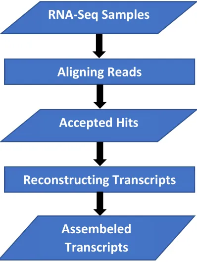
5.2.1 Genome mapping and transcriptome assembly . . . 107
5.2.2 Finding differentially expressed transcripts . . . 107
5.3 Results . . . 110
5.3.1 Malignant versus matched normal comparison . . . 110
5.4 Conclusion and discussion . . . 115
Bibliography . . . 123
6 Conclusion and future work 128 6.1 Conclusion . . . 128
6.2 Future work . . . 130
Bibliography . . . 132
A Clustering time-series profiles using wavelet based probability density functions (PDF) for identifying patterns in time series 134 A.1 The proposed clustering method . . . 134
A.1.1 Wavelet-based density function estimation . . . 135
A.1.2 The multi-level thresholding method . . . 136
A.1.3 Forward feature selection with memory . . . 136
Bibliography . . . 138
B The clinical and sequencing details of the Chinese prostate cancer dataset 139
C The clinical and sequencing details of the North American prostate cancer dataset 146
List of Figures
1.1 Central dogma of molecular biology. . . 2
1.2 Alternative splicing allows a gene to transcribe into two or more different ways using different
combinations of exons to produce different proteins. . . 3
1.3 TNM stages of prostate cancer. Courtesy: Comprehensive Urology [5]. . . 4
1.4 Gleason score patterns which was drawn by Dr. Gleason Courtesy: [3]. . . 5
1.5 The new breast cancer 10 subtypes clinical courtesy: [10], Kaplan–Meier plot of 15-years breast
cancer survival for each InClust. . . 9
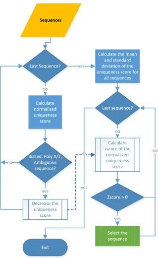
2.1 Schematic representation of the process for filtering reads using the Zseq method. . . 21
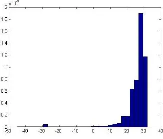
2.2 Distribution of the normalized uniqueness scores for all reads in sample (SRR202054) (µ=
25.8169, σ= 7.1681). . . 22
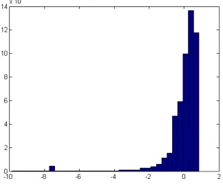
2.3 Distribution of the z-scores of the normalized uniqueness scores corresponding to each read
for sample (SRR202054). . . 24
2.4 Percentage of GC content for all filtered reads using the Zseq histogram (a) withµ= 52.63%
andσ= 12.08%. . . 26
2.5 Percentage of GC content for all filtered reads using the DUST histogram with µ= 53.09%
andσ= 12.36%. . . 26
2.6 Biologically meaningful human genomic sequences found using BLAST. De novo assembled
transcripts using original reads. . . 28
2.7 Biologically meaningful human genomic sequences found using BLAST. De novo assembled
transcripts using reads filtered by DUST. . . 28
2.8 Biologically meaningful human genomic sequences found using BLAST. De novo assembled
transcripts using reads filtered by Zseq. . . 29
2.9 An example of two transcripts, one with separable FPKM values (a), and another transcript
with inseparable FPKM values (b). . . 30
3.1 Preprocessing pipeline for each sample in the data set. . . 41
3.2 The 19,698 interpolated transcript profiles, each profile consists of the log(FPKM) values of
the transcripts expressions throughout prostate cancer stages/sub-stages(a), the profiles after
universal alignment(b). . . 44
3.3 PAAC values for the proposed method for the first data set. . . 46
3.4 PAAC values for the hierarchical clustering based on Euclidean distance for the first data set. 46
3.5 PAAC values for the proposed method for the second data set. . . 47
3.6 PAAC values for the hierarchical clustering based on Euclidean distance for the second data
set. . . 47
3.7 The first dataset: cluster 2 - main cluster for the proposed method. . . 48
3.8 The first dataset: cluster 2 - main cluster for the hierarchical clustering based on Euclidean
distance method. . . 48
3.9 The first dataset: clusters 1 to 16 of 31 distinct clusters detected by our proposed model. . . 49
3.10 The first dataset: clusters 17 to 31 of 31 distinct clusters detected by our proposed model. . 50
3.11 The second dataset: clusters 1 to 12 of 20 distinct clusters detected by our proposed model. 51
3.13 Comparison of CAMK2G mRNA expression in prostate cancer cells mimicking prostate cancer progression. QRT-PCR was performed to determine relative mRNA expression of CAMK2G in the MNU series of prostate cancer cell lines that mimic early through to late stages of
progression (NA22, stage 1 ; NB14, stage 2; NB11, stage 3; and NB26, stage 4). ∗p <
0.05, n= 3. . . 55
3.14 CAMK2G -N M172171 transcript in the second dataset. . . 56
4.1 Multi-Class classification model with performance measures. . . 69
4.2 Box plots for the AKIP1 and ASAP1 genes in node number one and two, which show the mini-mum, first quartile, median, third quartile, and maximum gene expression values for each group of samples (‘DH’ vs. Rest) and (‘DR’ vs. Rest). . . 70
4.3 Circos plot for the biomarker genes in node number one for the Rest samples based on the correlation coefficient among genes expressions (p <0.05). . . 71
4.4 Local and global outliers. . . 73
4.5 Dataset pre-processing. . . 74
4.6 Work flow of baseline method. . . 77
4.7 Slicing the time series based on window size and step size. . . 77
4.8 Window size and step size. . . 78
4.9 Change in gene trend. . . 79
4.10 Workflow of ACTS . . . 81
4.11 Heatmap for 24 oncogenes. . . 85
4.12 Heatmap for 18 tumor suppressor genes. . . 85
5.1 - A Schematic view of the proposed workflow for finding differential transcripts between benign vs. malignant and across various stages of prostate cancer . . . 108
5.2 Genes corresponding to the differentially expressed transcripts identified in Kannan’s, Kim’s and Ren’s datasets. . . 111
5.3 Expression trend of matched normal versus malignant transcripts. . . 111
5.4 Performance of five different classifiers for matched normal versus malignant classification. . . 113
5.5 Stage-specific expression level of transcripts that have been selected based on their significant expression changes between stages T1c and T2. . . 118
5.6 Stage-specific expression level of transcripts that have been selected based on their significant expression changes between stages T2 and T2a. . . 119
5.7 Stage-specific expression level of transcripts that have been selected based on their significant expression changes between stages T2a and T2b. . . 120
5.8 Stage-specific expression level of transcripts that have been selected based on their significant expression changes between stages T2b and T2c. . . 120
5.9 Stage-specific expression level of transcripts that have been selected based on their significant expression changes between stages T2c and T3a. . . 121
5.10 Stage-specific expression level of transcripts that have been selected based on their significant expression changes between stages T3a and T3b. . . 121
List of Tables
2.1 Comparison of the results of applying Zseq on samples from the prostate cancer data set as a
result of applying DUST on the same samples. . . 27
2.2 Average mapping rate of transcripts using the data set generated by the original reads, reads filtered by DUST and reads filtered by Zseq. . . 29
2.3 the number of discriminative transcripts for each of the three data sets. . . 30
2.4 Some artifacts measurements of prostate cancer samples which were preprocessed by EC-Zseq. 31 2.5 the number of decisive transcripts for the data set that was pre-processed by EC-Zseq. . . 32
3.1 Tumor samples that are analyzed from the first dataset. . . 40
3.2 Staging and description of the prostate cancer patent cohort [18]. . . 42
3.3 Genes and transcripts that correspond to prostate cancer were clustered as outliers for the first dataset. . . 52
3.4 Genes and transcripts that correspond to prostate cancer were clustered as outliers for the second dataset. . . 53
4.1 Comparison of the proposed model with SVM-RBF and an existing model. . . 64
4.2 The Steps of the proposed model shows the biomarker genes and which class can be determined at each step. . . 65
4.3 Class list with the number of saples in each class . . . 67
4.4 Result of baseline method. . . 83
4.5 Results of ACTS method. . . 87
5.1 Datasets used in this study for malignant vs. normal analysis with the number of samples in each dataset. . . 107
5.2 Distribution of Long’s dataset samples in various stages of prostate cancer. . . 108
5.3 Differentially expressed transcripts identified in Kannan’s, Kim’s and Ren’s datasets. . . 112
5.4 Top transcripts that discriminate stages T2 and T2Aof prostate cancer. . . 114
5.5 Top transcripts that discriminate stages T2A and T2B of prostate cancer. . . 114
5.6 Top transcripts that discriminate stages T2B and T2C of prostate cancer. . . 114
5.7 Top transcripts that discriminate stages T2C and T3A of prostate cancer. . . 115
5.8 Top transcripts that discriminate stages T3A and T3B of prostate cancer. . . 115
5.9 Top transcripts that discriminate stages T2C and T3/T4of prostate cancer. . . 116
5.10 Comparison between CuffDiff and our feature-selection method for identifying differentially expressed transcripts between each pair of consecutive stages of prostate cancer. . . 117
6.1 List of biomarkers that have been extracted by our methods . . . 129
B.1 The details of the samples sequencing runs for the Chinese dataset. . . 139
List of Symbols and Abbreviations
Symbol Definition
DN A Deoxyribonucleic Acid
RN A Ribonucleic Acid
RN A−seq RNA Sequencing
W HO World Health Organization
T N M Tumor, Node, and Metastases
mRN A messenger RNA
miRN A micro RNA
CN V Copy Number Variation
CN A Copy Number Aberration
N GS Next-generation Sequencing
SV M Support Vector Machine
k−N N k−Nearest Neighbors Algorithm
RBF Radial Basis Function
bp Base Pair
GP U Graphic Processing Unit
T P U Tensor Processing Unit
ORF s Open Reading Frames
Chr. Chromosome
Chr. Chromosome
P IN Prostatic Intra-epithelial Neoplasia
KSF Keratinocyte Serum Free
AU C Area Under Curve
V CD Variation Co-expression Detection
DB−index Davies-Bouldin’s index
M RI Magnetic Resonance Imaging
ACC Accuracy
F M F-Measure
Epigraph
Small stones together build a mountain
Chapter 1
Introduction
1.1
Transcriptome
Molecular biology is a branch of biochemistry that studies the molecular basis of biological
activity among biomolecules in a cell, such as the synthesis of DNA to RNA, and then to
proteins, as well as the regulatory mechanisms of the products of the genes. DNA is the
material that holds heredity information. Stored in the nucleus of the cell, it is arranged
into regions called chromosomes, which carry the genes. Each gene consists of a long chain
of nucleotides which is designated to perform a specific function. Roughly speaking, a gene
transcribes into mRNA, which then translates into protein. Nonetheless, some parts of the
gene “splice out” – called introns, while the remaining parts –coding parts or exons– “splice
into” messenger RNA, out of which a portion is translated into protein. Transcription and
translation are one-way direction processes as depicted in Figure 1.1; they form what is known
as the central dogma of molecular biology. Based on the fact that different transcripts for
specific genes may lead to a different protein, we decided to analyze the gene expression and
quantification on both gene level as in Chapter 4, and more detailed on the transcription
level as in Chapters 2, 3, and 5.
The transcriptome or usually known as all RNAs is the repertoire of all DNA molecules
that transcribe into RNA and the events that are associated with the transcription
DNA
RNA
Protein
Replication
Transcription
Translation
Figure 1.1: Central dogma of molecular biology.
alterations, transcriptome analysis opens the door for studying a number of external
fac-tors involved in gene expression such as environmental conditions, regulatory proteins, gene
transport, and others. The transcriptome includes the gene transcript expression profiling
and alternative splicing activity. It comprehensively includes the overall messenger RNA
(mRNA) expression in one cell, which is also known as single-cell transcriptome. Alternative
splicing is a regulated process during gene expression that results in coding multiple variants
or isoforms of RNA, which are then tranlated into different proteins via open reading frames
(ORFs). In this process, particular exons of a gene may be included within or excluded from
the final transcript (processed mRNA produced from that gene) [1]. Figure 1.2 depicts two
different scenarios of transcriptions of the same gene to form two different proteins.
1.2
Cancer
Cancer is a very complex disease that can be defined as unusual growth of cells. The
defining feature of this disease is the rapid creation of abnormal cells that grow beyond
their usual boundaries. According to the World Health Organization (WHO), cancer is the
second leading cause of death world-wide [2]. Cancer starts by transforming healthy cells
into tumor cells in a multistage process that generally progresses from a pre-cancerous lesion
Exon 1 Exon 2 Exon 3 Exon 4
Exon 1 Exon 2 Exon 3 Exon 4
Exon 1 Exon 2 Exon 3 Exon 1 Exon 2 Exon 4
Protein A Protein B
Gene
Transcript 2 Transcript 1
Figure 1.2: Alternative splicing allows a gene to transcribe into two or more different ways using different combinations of exons to produce different proteins.
genetic factors and three categories of external agents, including but not limited to:
• physical carcinogens agents, such as ultraviolet and ionizing radiation.
• chemical carcinogens agents, such as asbestos, components of tobacco smoke, aflatoxin
(a food contaminant), and arsenic (a drinking water contaminant).
• biological carcinogens agents, such as infections from certain viruses, bacteria, or
para-sites [2].
Similarly, the staging cancer system was devised by Pierre Denoix to notate the
differ-ent stages of cancer while progression takes place [4]. This notation system is known as
Classification of Malignant Tumors (TNM), where:
• T describes the size of the primary tumor and whether it has invaded nearby tissue.
Figure 1.3: TNM stages of prostate cancer. Courtesy: Comprehensive Urology [5].
• M describes distant metastasis, namely, how cancer spreads from one organ of the body
to another distant organ.
In Chapter 3, we present an approach that is used to quantify transcript reads over TNM
classification to interpolate the progression for prostate cancer tumours. More details about
the stages and the sub-stages of the samples are included in that chapter. Figure 1.3 depicts
the normal and different TNM stages of prostate tissues.
Prostate is a gland in the male reproductive system, and prostate cancer is the
develop-ment of cancerous cells in the prostate. While the majority of prostate cancers metastasize
very slowly, some metastasize very fast [6]. The aggressiveness of prostate cancer can be
measured using Gleason score. Gleason score is a grading system which was introduced by
Figure 1.4: Gleason score patterns which was drawn by Dr. Gleason Courtesy: [3].
appearance. The pathologist can determine the score based on collecting several details such
as tumor’s shape, tumor size, and which prostate tissue the tumor exists. The higher score
indicates greater risks and higher mortality. Cell morphology determines the structure, the
size, and how the shape of cells looks like such as cocci, bacilli, spiral shapes. The cancer
can be dominant or non dominant cell morphology in specific tissue based on whether or
not the majority of cells are cancer. The pathologist grade the dominant cell morphology
from 1 to 5 , and another score from 1 to 5 for the non dominant cell morphology. The total
addition of the two score form the total Gleason score that ranges from 2 to 10. Figure 1.4
depicts the Gleason scale patterns that pathologist can use to determine the score for both
dominant and non-dominant cell morphology.
Gleason score (pattern) descriptions are the following:
• Gleason pattern 1: is the most well-differentiated tumor pattern. It is a well-defined
nodule of single/separate, closely/densely packed, back-to-back gland pattern that does
shaped and proportionally large, when comparing them to those of Gleason pattern 3
tumors.
• Gleason 2: is fairly well circumscribed nodule of single, separate glands. However, the
glands are looser in arrangement and not as uniform as in pattern 1. Minimal invasion
by neoplastic glands into the surrounding healthy prostate tissue may be seen. Similar
to Gleason 1, the glands are usually larger than those of Gleason 3 patterns, and are
round to oval in shape. Thus the main difference between Gleason 1 and 2 is the density
of packing of the glands seen and invasion is possible in Gleason 2, not in Gleason 1 by
definition.
• Gleason pattern 3: is a clearly infiltrative neoplasm, with extension into adjacent
healthy prostate tissue. The glands vary in size and shape and are often long/angular.
They are usually small to medium size/micro-glandular in comparison to Gleason 1-2
grades. The small glands of Gleason 3, in comparison to the small and poorly defined
glands of pattern 4, are distinct glandular units.
• Gleason pattern 4: glands are no longer single/separated glands similar to those seen
in patterns 1-3. They look fused together, difficult to distinguish, with rare lumen
formation compared to Gleason 1-3 which usually all have open lumens (spaces) within
the glands, or they can be cribriform-(denoting an anatomical structure that is pierced
by numerous small holes. Resembling the cribriform plate/similar to a sieve. An item
with many perforations). Fused glands are chains, nests, or groups of glands that are
no longer entirely separated by stroma. Fused glands contain occasional stroma giving
the appearance of partial separation of the glands.
• Gleason pattern 5: Neoplasms have no glandular differentiation (thus not resembling
normal prostate tissue at all). It contains sheets (groups of cells almost planar in
appearance (similar to the top of a box), solid cords, or individual cells [7].
Gleason scores are often grouped based on similar behavior: Grade 2-4 being
-poorly differentiated grade neoplasm, and Grade 8-10 high-grade neoplasm. We have
de-veloped a machine learning approaches to obtain markers for prostate cancer Gleason score
[8]and laterality (location in the tissue) [9].
On the other hand, breast cancer is the most common type of cancer in female population
worldwide [2]. Breast cancer can be classified using the TNM classification and molecular
subtypes. In Chapter 4, we present an approach used to analyze the gene expression of
breast cancer patients to find markers that are related to specific subtypes using supervised
machine learning methods.
The tumor tissue under the microscope suggest nonlinear structure which is known as
tumor heterogeneity. Heterogeneity may show distinct morphological and phenotypic
pro-files, including cellular morphology, gene expression, proliferation, metabolism, motility, and
metastatic potential. Tumor heterogeneity has been observed in many type of cancer, breast
and prostate cancers are not any exception [16]. Targeting heterogeneity for furthur
anal-ysis can be in experimental and computational side, single cell sequencing and bulk tumor
sequencing can be both applied in the coputational side; In the first, an indicual cell can
be entirely sequenced amd the mutational profiles for distict cells can be analyzed with no
ambguity. However, this method is lacking of sufficient number of cells to obtain
statisti-cal significance. While in the bulk tumor sequencing, identifying rare mutations is difficult
because of the low frequency in the (bulk) mixture of cells.
Perou and colleagues categorized the molecular subtypes of breast cancer based on the
relative expression of 500 differentially expressed genes [17, 18], the five intrinsic categories
including:
• Luminal A breast cancer is hormone-receptor-positive (estrogen-receptor and/or
progesterone-receptor positive), HER2 negative.
• Luminal B breast cancer is hormone-receptor-positive (estrogen-receptor and/or
progesterone-receptor positive), and either HER2 positive or HER2 negative with high levels of Ki-67.
and progesterone-receptor negative) and HER2 negative.
• HER2-enriched breast cancer is hormone-receptor-negative (estrogen-receptor and
progesterone-receptor negative) and HER2 positive.
• Normal-like breast cancer is similar to luminal A, but is hormone-receptor positive
(estrogen-receptor and/or progesterone-receptor positive), and HER2 negative.
A recent research has introduced 10 molecular subtypes of Breast Cancer [10]. The aim of
this new subtype categorization is to obtain more separation in the largest subgroup of breast
cancer. In the 70% of breast cancers that are classified as estrogen-receptor
positive/HER2-negative in Luminal A, there is a tremendous heterogeneity; some groups of those patients
have different prognosis than others [13]. The genomic variation at a specific locus can lead
to a different expression for that gene. Curtis et al. generated a map of CNAs, CNVs,
and SNP for the new breast cancer classes. The integrative 10 classes which are named
InClust 1-10 have different clinical outcomes. Figure 1.5 shows the number of patients in
each InClust followed by the number of death from the specific disease between brackets
from the study [10].
1.3
Microarray
Chang et al introduced the microarray as anti-body microarray in 1983 [11]. In 1995, Schena
et al. used the microarray to monitor the expression of genes in parallel by reading
comple-mentary DNAs on glass using high-speed printing robotics [12]. After that, the microarray
industry established itself as the most used technology for reading gene expression with many
different industrial leaders in the market such as Affymetrix, Agilent, Applied Microarrays,
Arrayjet, Illumina, and others.
Microarray is capable to read the expressions of thousands of genes at the same time. a
microscope slides which known as DNA chips are positions to measure the gene expression
at the mRNA level that is known as transcriptome. Two mRNA samples, one from normal
Figure 1.5: The new breast cancer 10 subtypes clinical courtesy: [10], Kaplan–Meier plot of 15-years breast cancer survival for each InClust.
other disease, are converted into complementary DNA (cDNA). if a gene from both samples
have a similar expression, the corresponding chip will appear as yellow, if the experiment
gene has expressed less than the reference gene, the correspondence chip will appear as red,
1.4
Next-generation sequencing
Next generation sequencing (NGS) technology allows us to sequence the molecular events
fast at a very low cost, as well as higher sample throughput. The applications of NGS in
transcriptome analysis are commonly known as RNA Sequencing or RNA-Seq. There are
two main methods used to reconstruct the gene transcripts from sequenced reads. The first
one consists of comparing the reads to the reference genome for the same organism or a
similar known organism, while the second one consists of reconstructing the transcription
data from the reads without comparing it to known reference genome, which is known as de
novo assembly. Both techniques have been used in this thesis – see Chapter 2.
1.5
Machine learning
Machine learning is a branch of computer science that uses mathematical, statistical, and
logical techniques to make the machine learn from data without being programmed. In 1959,
Arthur Samuel came up with the name machine learning by combining artificial intelligence
in gaming and pattern recognition algorithms to make the machine learn from previous
experience. Data-driven predictions or decisions are the main purpose of machine learning.
Ever since, machine learning has evolved to include more applications and more challenges
to overcome by the machine including:
• Supervised learning, which means making the machine learn from labeled samples to
build the ability to predict or classify new unlabeled samples. Supervised learning
mainly includes classification and regression. We used these techniques in Chapters 2,
4, and 5.
• Unsupervised learning, in which the samples are not labeled, and hence, the machine
will attempt to group the samples based on similarities among them. Clustering is the
most popular application of unsupervised learning. In Chapter 3, we have contributed
outliers from time-series transcriptomic profiles. We further enhanced this algorithm
by extending the proposed method – see Chapter 4.
• Semi-supervised learning: since labeling samples is an expensive process, it starts with
labeling small number of samples, and then use the rest of the unlabeled samples in the
learning (training phase) which is more economically feasible. Mixing the unsupervised
techniques on the unlabeled data with the supervised techniques on both labeled and
unlabeled samples is a common technique in industry. The conjunction of labeled and
unlabeled samples may improve the accuracy of the learning system [14].
• Feature selection and extraction techniques are used to select or extract the most
infor-mative features (attributes) of the data that are relevant to the classification problem
that we are trying to solve. This includes feature selection (such as filter, wrapper, and
hybrid techniques), feature extraction, and dimensionality reduction techniques.
• Artificial neural network (ANN) and deep learning: In the attempt to mimic human
biological neural learning process, computer scientists created learning algorithms based
on connected nodes that can learn by forward propagation from the input layer to the
output layer going through the hidden layer. The nodes in the hidden layers have a
learning functions which is also known as activation functions. The nodes are connected
using weighted edges, which can be updated in the network back propagation phase to
reduce the error of the learning.
• Deep learning: A deeper neural networks or a neural network with multiple hidden layers
which recently emerge due to the revolutionary development in computer resources, such
as graphic processing units (GPU), and tensor processing unit (TPU). The complicated
deeper network are becoming more practical to optimize the machine learning; unlike
the ealier version of ANN, deep learning is about building multi-hidden layers of learning
rather than trying to understand the way that human brain works, which is known as
neuroscience technology [15].
time order. Time series applications exist in our daily life, including financial stocks,
weather forecast, heart beat rate, speech, and others. In scientific domains, time series
applications almost exist in all fields such as signal processing, earthquake prediction
and astronomy.
1.6
RNA-Seq preprocessing
NGS technology generates a large number of reads (short sequences), which contain a vast
amount of genomic data. The sequencing process, however, comes with artifacts such as
biased sequences, sequence duplications, and ambiguous nucleotides. Preprocessing of the
sequences is mandatory for further downstream analysis. In Chapter 2, we present Zseq,
a linear time method that identifies the most informative genomic sequences and de-rank
the sequences with artifacts. The complexity of a word in any language is that have
non-repetitive terms, so the word cat has a high complexity and most likely to be a word, while
cacacaca has a low complexity and most likely not to be a word in English language. In
order to measure the complexity of RNA sequences, Zseq calculates the complexity of the
sequences by counting the number of unique k-mers in each sequence as its corresponding
score and also takes into the account other factors such as ambiguous nucleotides or high
GC-content percentage in k-mers. Based on a z-score threshold, Zseq sweeps through the
sequences again and filters those with a z-score less than the user-defined threshold.
The Zseq algorithm is able to provide a better mapping rate; it reduces the number of
ambiguous bases significantly in comparison with other methods. Evaluation of the filtered
reads has been conducted by aligning the reads and assembling the transcripts using the
reference genome as well as de novo assembly. The assembled transcripts show a better
discriminative ability to separate cancer and normal samples in comparison with another
state-of-the-art method in Chapter 2. Moreover, de novo assembled transcripts from the
reads filtered by Zseq have longer genomic sequences than other tested methods. Estimating
results.
1.7
Outlier detection from time-series cancer RNA-Seq data
Studying the abundance of selected mRNA species throughout prostate cancer progression
may provide insight into the molecular mechanisms that advance the disease. In Chapter 3,
we reveal that the combination of proper clustering, distance function and index validation
for clusters are suitable in identifying outlier transcripts, which exhibit different trends than
the majority of the transcripts. Unlike an earlier works in which we clustered the profiles
to find patterns as illustrated in Appendix A, this work focuses on finding the trend of
a transcript is the abundance throughout different stages of prostate cancer. In modeling
cancer progression, the stages are represented as time points, and the increase in transcript
abundance throughout those time points are cubic-spline interpolated. After profiling the
transcripts, we universally aligned the profile to a coordinate profile z [47], then we
hierar-chically clustered the profiles to find outliers profiles that have large distances and differently
trend than the other profiles.
Using a hierarchical clustering method for time-series profile data, we identified
stage-specific mRNA species termed outlier transcripts that exhibit unique trending patterns as
compared to most other transcripts during disease progression. This method is able to
identify those outliers rather than finding patterns among the trending transcripts compared
to the hierarchical clustering method that is based on the Euclidean distance. Our proposed
algorithm was able to identify the outliers and cluster them in singleton-clusters or in clusters
containing a small number of transcripts, while the hierarchical clustering based on Euclidean
distance was trying to find patterns rather than exclude the outliers.
A wet-lab experiment on a marker gene CAMK2G confirmed the results of the
com-putational model on a dataset of samples from a Chinese population. Genes related to
these outlier transcripts were found to be strongly associated with cancer, and in particular,
may identify them as potential stage-specific indicators that can predict disease progression,
leading to novel drugs or therapies.
Studying gene expression through various time intervals of breast cancer survivability may
provide deeper insight into the recovery of the patients. Gene expression values are different
in various stages of progression of the disease. Discovery of gene biomarkers can be a crucial
step in predicting survivability and handling breast cancer patients. In Chapter 4, we present
an approach used to enhance a hierarchical clustering method to separate dissimilar groups
of genes in time-series data as outliers. These isolated outliers (genes that trend differently
from other genes) can serve as potential markers of breast cancer survivability. Noise is
undesirable case or unwanted case in data distribution, the noise can be generated randomly
or non-randomly. Outliers are cases who are removed from the main body of the data, where
the proximities of the outlier to the other cases are generaly small, in another words, the
measurment of the outlier is away from the mean of the other measurements in the same
class [21]. In supervised learning, the outlier can be determined by identifying the border of
the class using support vector machines [21] or anti-Bayesian [22]; this technique known as
one class classification.
Outliers can be studied to analyse unusual situation since the outlier can be a legitimate
case, while it is usually treated as noise or error in a measurment. It also may introduce
novelty in any distribution. Since cancer is unusual growth of the cells, unusual growth of
the cancerous cells over time needs to be carefully studied to analyze the nature of cancer,
in addition to the motives of the expression at some certain time points.
We partition the time axis (time points) into bins of length six months starting from 1-6
up to 55 months intervals and, for each gene, we average its expression level over all patients
who appear in a survival bin. Gene expressions throughout those time points are cubic
spline interpolated to create a trending profile for each gene. First, we universally align the
gene expression profiles to minimize the total area between them. Then, we cluster them
using a sliding window approach and hierarchical clustering based on minimum squared error
To the best of our knowledge, this work is the first time-series model that is built on the
survival time of patients after the treatment. With this approach, we identified 60 genes
(including 36 oncogenes and 18 tumor suppressor genes) as potential biomarkers of breast
Bibliography
[1] Douglas L Black. Mechanisms of alternative pre-messenger rna splicing. Annual review
of biochemistry, 72(1):291–336, 2003.
[2] World Health Orgnization. Cancer. http://www.who.int/, 2018. [Online; accessed
19-April-2018].
[3] Donald F Gleason. The Veteran’s Administration Cooperative Urologic Research Group:
histologic grading and clinical staging of prostatic carcinoma. Lea and Febiger, 1977.
[4] Pierre F Denoix. Enquete permanent dans les centres anticancereux. Bull Inst Nat Hyg,
5(1):1–70, 1946.
[5] Comprehensive Urology. Stages of Prostate Cancer. https://
comprehensive-urology.com/basics-of-prostate-cancer-grading-and-staging/,
2018. [Online; accessed 19-April-2018].
[6] World Health Organization. World Cancer Report, volume 5. World Health
Organiza-tion, 2014.
[7] Jonathan I Epstein, William C Allsbrook Jr, Mahul B Amin, Lars L Egevad, ISUP
Grad-ing Committee, et al. The 2005 international society of urological pathology (isup)
con-sensus conference on gleason grading of prostatic carcinoma. The American journal of
surgical pathology, 29(9):1228–1242, 2005.
[8] Osama Hamzeh, Abedalrhman Alkhateeb, Iman Rezaeian, Aram Karkar, and Luis
generation sequencing and machine learning techniques. InInternational Conference on
Bioinformatics and Biomedical Engineering, pages 337–348. Springer, 2017.
[9] Osama Hamzeh, Abedalrhman Alkhateeb, and Luis Rueda. Predicting tumor locations
in prostate cancer tissue using gene expression. In International Conference on
Bioin-formatics and Biomedical Engineering, pages 343–351. Springer, 2018.
[10] Christina Curtis, Sohrab P Shah, Suet-Feung Chin, Gulisa Turashvili, Oscar M Rueda,
Mark J Dunning, Doug Speed, Andy G Lynch, Shamith Samarajiwa, Yinyin Yuan,
et al. The genomic and transcriptomic architecture of 2,000 breast tumours reveals
novel subgroups. Nature, 486(7403):346, 2012.
[11] Tse-Wen Chang. Binding of cells to matrixes of distinct antibodies coated on solid
surface. Journal of immunological methods, 65(1-2):217–223, 1983.
[12] Mark Schena, Dari Shalon, Ronald W Davis, and Patrick O Brown. Quantitative
mon-itoring of gene expression patterns with a complementary dna microarray. Science,
270(5235):467–470, 1995.
[13] Medscape New Map of Breast Cancer Identifies 10 Disease Subtypes. https://www.
medscape.com/viewarticle/762239#vp_2, 2018. [Online; accessed 14-May-2018].
[14] Kamal P Nigam. Using unlabeled data to improve text classification. Technical
re-port, CARNEGIE-MELLON UNIV PITTSBURGH PA SCHOOL OF COMPUTER
SCIENCE, 2001.
[15] Yann LeCun, Yoshua Bengio, and Geoffrey Hinton. Deep learning. nature,
521(7553):436, 2015.
[16] Andriy Marusyk and Kornelia Polyak. Tumor heterogeneity: causes and consequences.
Biochimica et Biophysica Acta (BBA)-Reviews on Cancer, 1805(1):105–117, 2010.
[17] Charles M Perou, Therese Sørlie, Michael B Eisen, Matt Van De Rijn, Stefanie S Jeffrey,
Christian A Rees, Jonathan R Pollack, Douglas T Ross, Hilde Johnsen, Lars A Akslen,
[18] Aleix Prat and Charles M Perou. Deconstructing the molecular portraits of breast
cancer. Molecular oncology, 5(1):5–23, 2011.
[19] Numanul Subhani, Luis Rueda, Alioune Ngom, and Conrad J Burden. Multiple gene
expression profile alignment for microarray time-series data clustering. Bioinformatics,
26(18):2281–2288, 2010.
[20] Leo Breiman. Random forests. Machine learning, 45(1):5–32, 2001.
[21] Vladimir Naumovich Vapnik. The nature of statistical learning theory, ser. statistics for
engineering and information science. New York: Springer, 21(1003-1008):2, 2000.
[22] Yifeng Li, B John Oommen, Alioune Ngom, and Luis Rueda. Pattern classification using
a new border identification paradigm: The nearest border technique. Neurocomputing,
Chapter 2
Zseq : an approach for preprocessing
next generation sequencing data
2.1
Introduction
A low-complexity sequence of nucleotides has highly biased distribution of nucleotides in a
way that makes the sequence less diverse of unique k-mers of nucleotides. The lower the
complexity of a sequence, the more likely that the sequence will be mapped to different parts
of the genome. In other words, when we process low-complex sequences, there is less chance
that we can align it to a specific part of the genome uniquely. This low level of certainty
regarding the real position of a sequence, makes it less desirable to be used.
Poly A/Poly T is a chain of A or T, used to prime the three and five sites in a genome
sequence during cDNA library preparation [6]. Poly A/T sequences may cause bias in the
reads. The intronic Poly A/T tails tend to splice out rather than staying between coding
exons [7]. The GC content represents the ratio of a G-C pair in the genome sequence. The
stop codons show a significantly high ratio of A-T nucleotides [8], while coding codons have
a higher GC content [9]. The GC content of a gene plays an important role in carrying
the genetic information. The GC content of the human genome varies among different
representation of A+T sequences can be significantly lower, because in the preparation of a
standard library a gel slice is used and heated up to 50◦C, thereby increasing the bias of the
GC content [11].
Fastqc can be used to check the quality of the sequenced reads that is coming from high
throughput sequencing pipelines. It provides a modular set of analyses wether your data
should be preprocessed and which kind of biases or artifacts which the raw data may have
at each base pair position in the reads [12]. Fastqc can works FASTA and FASTQ format
where both are similar except that FASTQ provides a quality measurment of each sequenced
base pair. Fastqc is useful to view the content of the data before and after preprocessing the
sequences using tools such as Zseq.
There are different techniques that try to remove those sequences with low-complexity
patterns from samples. Morgulis et al. presented the symmetric DUST method [13], which
masks low-complexity regions in a sequence to overcome context sensitivity in calculating
the complexity score. Schmieder et al. proposed two methods to evaluate the sequence
complexity [14]. The first method is based on entropy as a measure. The second method,
which is a variant of the DUST algorithm based on BLAST search, filters out the
low-complexity score sequences. Both methods consider each triplet of nucleotides as a word.
One of the downsides of the previous methods is that they focus only on the complexity
of the sequences. This can be misleading in some cases due to the highly biased nature
of the sequences. In this chapter, we propose a novel method called Zseq, which decreases
the uniqueness score of highly biased regions, thereby filtering highly biased sequences and
low-complexity sequences.
2.1.1 Methods
Figure 2.1 depicts the process of finding reads with improved quality. Each module is
ex-plained in detail in the next few paragraphs.
In the first step, Zseq scans all the reads and calculates the uniqueness score for all reads.
Figure 2.1: Schematic representation of the process for filtering reads using the Zseq method.
that read. Zseq considers the defaultk-mer size,w, as 4-mers, which makes the vocabulary of
four nucleotides (A,T,C,G) to be 44 = 256 words. As the long reads may contain thousands
Figure 2.2: Distribution of the normalized uniqueness scores for all reads in sample (SRR202054) (µ =
25.8169, σ= 7.1681).
is because a 3-mer word can exist many times in the same read without being considered as
unique, even when it is associated with different nucleotides each time. Zseq excludes the
5-mers of the low-complex/biased artifacts, such as ambiguous bases (N), PolyA/T and GC
content, from being unique by decreasing the unique score of the reads by one for each 2w
in order to reduce the chances of selecting this sequence later. The uniqueness score of each
read is then normalized by dividing it by the length of the read. The normalized uniqueness
scores of all reads are stored in a vector with the same order of the read in the input file.
Figure 2.2 shows the distribution of the normalized uniqueness scores for all reads for sample
SRR202054 from the prostate cancer data set used in the study of [16]. The x-axis shows
the normalized uniqueness scores, while the y-axis shows the number of reads. As shown in
the figure, the penalized sequences have a very small score down to -30. These are sequences
that have been generated using reads that contain long PolyA/T sequences, very high GC
In the next step, Zseq calculates the mean and standard deviation for the normalized
uniqueness scores. The mean of the normalized uniqueness scores of all reads is calculated
in the first loop. The variance is also calculated linearly using a Na¨ıve algorithm to reduce
the cost of this step. The standard deviation is calculated from the variance of the vector of
the normalized uniqueness scores.
Next, for each normalized uniqueness score, we calculate the z-score using the mean, µ,
and the standard deviation, σ, as follows:
z = (s−µ)/σ. (2.1)
The z-score represents how many standard deviations the normalized uniqueness score of
the read is away from the mean µ for all normalized uniqueness scores. In other words, if
a read has a z-score of 0, it means that the read has the normalized uniqueness score of µ,
while a z-score of value 1 means that the normalized uniqueness score is away exactly one
standard deviation from the µ. Figure 2.3 shows the z-scores for all reads in the sample
(SRR202054), where the x-axis is thez-score of the normalized uniqueness scores, while the
y-axis indicates how many reads a particular z-score has in the sample.
Finally, the user-adjustable threshold θ is used to determine whether or not to select the
reads, if the z-score of the normalized uniqueness score of the reads is greater than or equal
toθ, the read will be selected; otherwise, it will be filtered out.
2.1.2 Estimating the cuttoff point
A data driven method based on the labeling rules is used to filter out the reads with low
uniqueness score. The method automatically finds the cutoff pointcto compensate θ in the
histogram of reads’ uniqueness scores and removes those reads whose uniqueness score is less
than c. The labeling rules model calculates the first quartile q1 and third quartile q3 using
cut-off point is calculated as follows:
c=q1−g(q3−q1) (2.2)
where g is the g-factor that can be calculated as follows:
g = (h−q1)/h (2.3)
withhbeing the highest value in the histogram of reads’ uniqueness scores. After calculating
the cut-off point c, the method sweeps again throughout the reads and selects those that
have uniqueness score ≤c
2.2
Results
In our experiments, we used the prostate cancer data set utilized in the study of [16]. The
data set is publicly available in NCBI Gene Expression Omnibus (GEO) under accession no.
GSE29155. It contains 11 samples in total, where seven of them belong to tumor tissues
and the remaining four samples are benign. We measured the GC content and the number
of ambiguous bases of the outcomes of each method, and then aligned the results of both
methods to the human genome using Tophat2 as the alignment method [18].
DUST takes a value that ranges from 0 and 100 as the complexity threshold, while Zseq
takes a z-score value as a complexity threshold, which shows how many standard deviations
the normalized uniqueness score of the read is away from the mean. For the DUST method
we chose the value 5 as the threshold, which means that the value of the complexity of the
read has to be greater than or equal to 5 to be selected; otherwise, DUST will ignore the
read. For Zseq, we have chosen -1.5 as the value of the threshold, which makes the read
good to be selected if the z-score of that read is greater than or equal to -1.5. The reason
behind selecting these two thresholds is that both methods filter almost the same number of
reads in each sample.
Figure 2.4: Percentage of GC content for all filtered reads using the Zseq histogram (a) with µ= 52.63%
andσ= 12.08%.
Figure 2.5: Percentage of GC content for all filtered reads using the DUST histogram withµ= 53.09% and
σ= 12.36%.
also has smaller standard deviation which makes the reads centered more around the mean
than DUST. Figure 2.4 and Figure 2.5show the GC content distributions for both methods
applied on the same sample set (SRR202058).
Zseq shows a slight improvement in reducing the GC content, mapping rate and mapping
time, while dropping the number of ambiguous bases drastically in comparison with DUST.
Table 2.1 shows that the number of ambiguous bases, N, in the filtered reads using Zseq have
drastically decreased compared with the ambiguous bases that have been filtered out using

![Figure 1.3: TNM stages of prostate cancer. Courtesy: Comprehensive Urology [5].](https://thumb-us.123doks.com/thumbv2/123dok_us/1344897.1167349/25.612.85.532.76.423/figure-tnm-stages-prostate-cancer-courtesy-comprehensive-urology.webp)
![Figure 1.4: Gleason score patterns which was drawn by Dr. Gleason Courtesy: [3].](https://thumb-us.123doks.com/thumbv2/123dok_us/1344897.1167349/26.612.74.543.68.359/figure-gleason-score-patterns-drawn-dr-gleason-courtesy.webp)
![Figure 1.5: The new breast cancer 10 subtypes clinical courtesy: [10], Kaplan–Meier plot of 15-years breastcancer survival for each InClust.](https://thumb-us.123doks.com/thumbv2/123dok_us/1344897.1167349/30.612.73.522.77.569/figure-subtypes-clinical-courtesy-kaplan-breastcancer-survival-inclust.webp)
![Table 3.2: Staging and description of the prostate cancer patent cohort [18].](https://thumb-us.123doks.com/thumbv2/123dok_us/1344897.1167349/63.612.189.419.282.515/table-staging-description-prostate-cancer-patent-cohort.webp)

