Electromechanically Coupled Finite Element Model of a Circular Electro-active Polymer Actuator.

ABSTRACT

DEODHAR, ASEEM PRALHAD. Electromechanically Coupled Finite Element (FE) Model of a Circular Electro-active Polymer Actuator. (Under the direction of Dr. Stefan Seelecke).

This thesis presents a Finite Element model of a circular Dielectric Electro-active Polymer

(DEAP) actuator using two different hyperelastic material models. This model is a first

approximation of the material behavior of the DEAP and lays out a basic framework of

modeling an electromechanically coupled DEAP as a system by neglecting the hysteric and

rate-dependent material behavior. This includes the modeling of the compliant electrodes

along with the polymeric dielectric. The compliant electrodes, pasted on both sides of the

elastomer, have a large effect on the mechanical behavior of the DEAP which needs to be

taken into consideration while modeling the DEAP system. The model is developed using the

commercial Finite Element Modeling software, COMSOL Multiphysics. The material

parameters are found by systematically varying them and comparing the simulation results to

known experimental results. The results from the mechanical simulations are presented in the

form of force-displacement curves and are validated by comparing them to experimental

results. Electromechanical simulations are carried out and the stroke of the actuator for

different electrode stiffness values is compared with experimental values when the DEAP is

biased with a constant force. The comparisons with experimental values are good

qualitatively. The capacitance variation of the DEAP as a function of deformation is also

predicted by the model and is in good agreement with the experimental values. This work

lays out a platform for further enhancements by including the viscoelastic material properties

Electromechanically Coupled Finite Element Model of a Circular Electro-active Polymer Actuator

by

Aseem Pralhad Deodhar

A thesis submitted to the Graduate Faculty of North Carolina State University

in partial fulfillment of the requirements for the degree of

Master of Science

Mechanical Engineering

Raleigh, North Carolina

2011

APPROVED BY:

_______________________________ ______________________________

Dr. Gregory Buckner Dr. Mohammed Zikry

________________________________

ii

DEDICATION

iii

BIOGRAPHY

Aseem Deodhar was born in Pune, India on August 10, 1986. He graduated as a Bachelor of

Technology in Mechanical Engineering in May 2008 from College of Engineering, Pune

iv

ACKNOWLEDGMENTS

I would like to thank my adviser Dr. Stefan Seelecke for all his patience with me and all the

guidance, motivation and encouragement. I also thank him for giving me an opportunity to

travel to Germany. It has been a great experience working with him.

I also thank Dr. Gregory Buckner and Dr. Mohammed Zikry for serving on my graduate

committee.

I would also like to thank Dr. Alexander York for all his help with the experimental data and

extremely useful tips about writing and presenting technical data. Special thanks to Micah

Hodgins for his help with experiments and simulations. I thank the other members (past and

present) of the Adaptive Structures Lab – Stephen Furst, Gheorghe Bunget, Rohan Hangekar

and Nicole Lewis for all the good times at and away from work.

I specially thank my cousin sister Mrunal and her husband Anant Natu for all their help and

support.

Finally, I‘m most thankful to my parents and my elder brother for all their love, support and

v

TABLE OF CONTENTS

LIST OF FIGURES ... vii

LIST OF TABLES ... ix

Chapter 1. INTRODUCTION ... 1

1.1 Introduction and Background ... 1

1.2 Literature Review ... 2

1.3 Motivation ... 4

1.4 Thesis Overview ... 5

Chapter 2. MECHANICS & ELECTROSTATICS ... 7

2.1 Problem Characterization ... 7

2.2 Hyperelastic Material Models ... 9

2.2.1 Neo-Hookean material model ... 10

2.2.2 Mooney-Rivlin material model ... 10

2.2.3 Determination of material parameters for Mooney-Rivlin material ... 11

Chapter 3. GEOMETRY & FE MODEL ... 14

3.1 Geometry of the DEAP actuator ... 14

3.2 Boundary Conditions... 15

3.2.1 Mechanical Boundary Conditions ... 18

3.2.2 Electrical Boundary Conditions... 19

3.2.3 Electromechanical Boundary condition ... 19

3.3 Finite Element Mesh ... 20

Chapter 4. MECHANICAL SIMULATIONS ... 23

4.1 Experiments ... 23

4.2 Simulations ... 25

4.2.1 Pre-strain ... 25

4.2.2 Solver ... 26

vi

Chapter 5. ELECTRO-MECHANICAL COUPLING ... 32

5.1 Experiments ... 32

5.2 Simulation Procedure ... 33

5.3 Results ... 34

5.3.1 Time Resolved Data ... 34

5.3.2 Local Results ... 35

5.3.2.1 Deformation and Stress ... 35

5.3.2.2 Electric Field ... 39

5.3.2.3 Charge Distribution ... 40

5.3.3 DEAP Stroke ... 40

5.3.4 Global Results... 42

5.3.4.1 Force-Voltage Characteristics ... 42

5.3.4.2 Capacitance Variation (Sensing Applications) ... 43

5.4 Simulations with a .75 inch2 actuator ... 44

5.5 Further Experiments ... 46

5.5.1 Electrode Thickness variation ... 46

5.5.2 Actuator diameter variation ... 47

CONCLUSIONS... 51

REFERENCES ... 52

APPENDICES ... 57

APPENDIX – 1 Basic Mechanics and Electrostatics... 58

A1.1 Deformation and Strain ... 58

A1.2 Stresses ... 60

A1.3 Electrostatics ... 61

vii

LIST OF FIGURES

Figure 1: DEAP construction and Operating principle ... 1

Figure 2: Sketch of a circular DEAP actuator. ... 2

Figure 3: Mechanical response of the elastomer without electrodes and with pasted electrodes. [33] ... 4

Figure 4: Stress - Strain diagram for Hookean, Neo-Hookean and Mooney-Rivlin material models. ... 11

Figure 5: DEAP actuator ... 14

Figure 6: Electroactive Polymer Actuator Geometry - Solidworks model [33]. ... 15

Figure 7: Pre-loading the DEAP in out-of-plane direction schematic. [33] ... 16

Figure 8: Simplified loading & boundary conditions ... 16

Figure 9: Mechanical Boundary Conditions ... 18

Figure 10: Electrical Boundary conditions ... 19

Figure 11: Vertical displacement at the edge marked red and radial stresses at points 1,2,3 for global and local mesh convergence respectively. ... 20

Figure 12: Global mesh convergence with uniform mesh (left) and non-uniform mesh (right). ... 21

Figure 13: Local mesh convergence with uniform mesh (left) and non-uniform mesh (right). ... 21

Figure 14: Finite Element mesh and a zoom in at the left end. [34] ... 22

Figure 15: Setup for tensile experiment on elastomer specimen ... 23

Figure 16: Stress vs Strain plot for simple tensile experiment on the elastomer. ... 24

Figure 17: Schematic for out-of-plane deformation experiments [33]. ... 24

Figure 18: Displacement Input in displacement control simulation. ... 28

Figure 19: Force vs Displacement curves for different values of elastomer Young's modulus. [34] ... 29

viii

Figure 21: Schematic for electro-mechanical experiments on the DEAP [33]. ... 32

Figure 22: Schematic of test setup (left) and the actual set-up (right). [34] ... 33

Figure 23: Time resolved data. Input parameters (top left), Displacement output (top right). Experimental displacement output for one voltage cycle (bottom). [34] ... 34

Figure 24: Time resolved data for Displacement control (Simulation – Top, Experimental – Bottom). ... 35

Figure 25: Deformation shapes of the elastomer during pre-deflection and actuation. [34] .. 36

Figure 26: Radial Stress Contour plots ... 37

Figure 27: Thickness Stresses Contour Plot ... 38

Figure 28: Electric Field Contour Plots ... 39

Figure 29: Surface Charge densities on the internal surface of the top electrode (left) and bottom electrode (right). ... 40

Figure 30: Test setup schematic (left) and actual picture of the test (right). [34] ... 41

Figure 31: Suspended Mass vs Stroke. ... 42

Figure 32: Blocking Force vs Voltage curve for fixed displacement of 2mm... 43

Figure 33: Capacitance variation with deformation... 44

Figure 34: Force v Displacement for DEAP75 actuator with electrodes ... 45

Figure 35: Force v Voltage plot for DEAP75 actuator ... 46

Figure 36: Variation of pre-deflection and radial stresses in electrodes with thickness ... 47

Figure 37: Variation of Stresses with change in actuator diameter DEAP75 (Top Left), DEAP100 (Top right), DEAP200 (Bottom). ... 48

Figure 38: Variation in capacitance with variation in diameter. Experimentally validated plot (top) and prediction for other geometries (bottom). ... 49

ix

LIST OF TABLES

Table 1: Material parameters for the two material models ... 27

1

Chapter 1. INTRODUCTION

1.1 Introduction and Background

The main focus of this thesis is to develop an electromechanically coupled, multi-field finite

element model of a circular Dielectric Electro-Active Polymer (DEAP). A DEAP is

essentially a capacitor with a compliant elastomer as the dielectric and compliant conducting

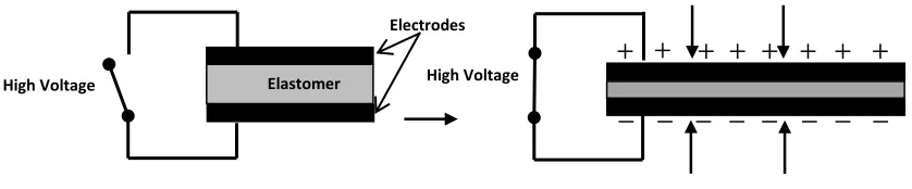
electrodes pasted on both sides. The basic construction is as shown in Figure 1. When a

potential difference is applied across the electrodes the electrostatic charges build up on the

electrodes and they attract each other. In the process they exert mechanical pressure on the

thin elastomeric dielectric and squeeze it between them. Due to the mechanical pressure, the

elastomer film contracts in the thickness direction and is enlarged in the in-plane directions.

DEAPs are actuated at high voltages (typically 2kV – 5kV) but draw very low current and

hence have low power consumption.

The DEAPs are also pre-deflected in order to use the strain caused by the electrostatic

(Maxwell‘s) force to produce displacement stroke. There are various DEAP configurations

being studied for different applications and there are a number of ways in which the DEAP

can be pre-deflected.

High Voltage Elastomer

Electrodes High Voltage

2

Figure 2: Sketch of a circular DEAP actuator.

Electroactive polymers (DEAP) are a novel variety of materials which can potentially be

used in active structures as actuators and sensors. With a large number of miniature

applications envisioned for DEAPs [1-7, 10], they are quickly becoming a primary focus of

research among industry and academia with various applications such as prosthetic devices,

braille display systems and flat panel loudspeakers, to name a few. There are several

properties of DEAP materials including low power consumption, high elastic energy density

[1], fast response [8], light-weight [9] and silent operation which make them an attractive

choice for use smart material systems and devices.

1.2 Literature Review

This section presents a review of some of the previous modeling and simulation work done

on Electroactive Polymer devices. It includes both the analytical models and finite element

models developed for various actuator geometries and configurations.

Pelrine et al [2] presented the mechanism of electrostriction in Electroactive Polymers due to

the electrostatic attraction of free charges on the electrodes. They derive relationships for the

effective actuation pressure of an DEAP. They found that this pressure is twice that in a

parallel plate capacitor and they attribute the excessive pressure to the compliance of the

electrodes. They also experimentally investigated the in-plane stresses for actuators made of

3

experimental values. Kofod [11] presented an electromechanically coupled model for DEAPs

using elastic and hyperelastic material models. The voltage-strain response was plotted for

each of the models with an applied weight to the DEAP. The Ogden [12] model predicted a

response which lied in between those of Hooke and Neo-Hooke models. Zhao [13] et. al

proposed an analytical model for a membrane of a dielectric elastomer deformed into an

out-of-plane axi-symmetric shape. Their model studies the kinematics of deformation and

charging, together with thermodynamics, leads to equations that govern the state of

equilibrium. Goulbourne [14] et al presented a method for modeling dielectric elastomer

membrane accounting for material non-linearity and large deformations. Their model is

tailored to axi-symmetric inflatable membranes, used in artificial blood pump systems.

Wissler [15, 23-24] et. al presented a considerable amount of work on modeling and

simulating the DEAP actuators. They simulated a pre-stretched circular DEAP actuator,

activated with a predefined voltage, using the commercially available FE software

ABAQUS. They propose a novel approach for FE analysis of elastomer actuators in which

they use kinematic boundary conditions to apply the electromechanical pressure. They found

discrepancies in the uni-axial test data from experiment and simulations due to the time

dependent material response. Rosenblatt [16] et. al present a technique to accurately model

DEAPs taking into account non-linearities and large deformations. They proposed an

algorithm to model the electromechanical coupling that is inherent to dielectric DEAP

systems. Their algorithm was validated by using finite element simulations with the

commercially available software ANSYS. Wissler [17] et. al investigated the

electromechanical coupling in dielectric EAPs. They analyzed the analytical equation of

electrostatic forces in dielectric elastomer systems with energy considerations and numerical

calculations. Their system was modeled using COMSOL, to plot charge and electrostatic

force distributions. Lochmater [18] et. al modeled the viscoelastic behavior of a dielectric

film using spring damper framework. The model predicted stable deformation state under

activation with constant charge and an unstable equilibrium state for activation under

constant voltage. Jung [19] et. al presented a computational system to describe

4

[20] and Yeoh [21] model are used for simulations in the commercial FE program ANSYS.

The predictions of the Mooney-Rivlin model showed good agreement with the experimental

data. Gao [22] et. al combined the hyperelastic Ogden material model with total Maxwell‘s

stress methods to describe the material. They also formulated large deformation Finite

Element models and compared simulation results to experimental results to validate the

computational model.

While all of these models provide beneficial insight into the elastomer material behavior

itself, they lack the ability to accurately predict a complete DEAP actuator structure which

includes compliant electrodes. Including these other elements into a coupled model is

necessary for behavior predictions of various DEAP actuators as they would be used in

commercial applications. The electrodes have a non-negligible effect on the mechanical

response of the DEAP which can be seen from the Figure 3 below.

Figure 3: Mechanical response of the elastomer without electrodes and with pasted electrodes. [33]

1.3 Motivation

As it is seen from the above figure, the force-displacement graphs plotted for the elastomer

with and without electrodes show that there is an appreciable difference in the mechanical -0.8

-0.7 -0.6 -0.5 -0.4 -0.3 -0.2 -0.1 0

0 0.5 1 1.5 2 2.5 3 3.5

Fo

rce

(

N

)

Displacement (mm)

Force vs. Displacement

Elastomer

5

response of the actuator for the two cases. It is clear from Figure 3 that the electrodes make

the actuator stiffer and add a considerable amount of hysteresis in the actuator response. The

focus of this work is to develop an electromechanically coupled finite element model which

takes into account the effect of electrodes in the mechanical response of the DEAP actuator.

There are challenges modeling an elastomeric polymer actuators resulting from their inherent

electromechanical coupling and non-linear and hysteretic material behavior. A finite element

model will also help in better design of the DEAP system geometry for specific applications.

The Finite Element (FE) also has to account for the electro-mechanical coupling that results due to the Maxwell‘s forces from the applied electric field inducing a mechanical

deformation as explained in section 1.1.

The finite element model presented in this work is developed using the commercial finite

element code COMSOL Multiphysics and is a first step towards a DEAP actuator system

model.

1.4 Thesis Overview

This thesis presents a Finite Element model of a DEAP actuator as a system taking into

account the influence of the electrodes on the mechanical performance of the actuator.

Chapter 2 lays out the basic partial differential equations governing the electromechanically

coupled problem. A brief introduction to the basic hyperelastic material models – Neo

Hookean and Mooney-Rivlin is also included in this chapter.

Chapter 3 introduces the geometry and the finite element model for the Electroactive

Polymer actuator. It describes the boundary conditions, and the finite element mesh used for

the simulations.

Chapter 4 and 5 describe the process of material parameter calibration for the material

models used. They present the simulation results and comparison with experimental values.

Chapter 5 also presents the validation of the model by simulating a different DEAP geometry

6 model predictions are also presented.

7

Chapter 2. MECHANICS & ELECTROSTATICS

This chapter describes the electromechanical problem formulation starting from the basic

momentum balance equations. A brief description of the hyperelastic materials is also

included.

2.1 Problem Characterization

The modeling of the DEAP system in a Finite Element program involves solving of the

partial differential equations that define each of the physics – mechanics, electrostatics and

electro-mechanical coupling.

The characterization of a structural mechanics problem involves specifying the balance

principles, the Neumann and the Dirichlet boundary conditions and the constitutive laws or

equations which presume the existence of a relation between forces and displacements with

stresses and strains respectively, which is exclusively local i.e. at the considered material

point.

The momentum balance principle describes the equilibrium of internal forces and stresses.

The forces on a body such as body loads, inertial forces and forces resulting from the

stresses. In tensor form the local balance of momentum can be stated as [29]:

u_i _{ij j,} b_i (1)

here, ρ is the density, u_iis the acceleration vector, _{ij j,} is the divergence of the Cauchy

Stress tensor and bi is the matrix of volume specific body loads. In case of a quasi-static

model, the acceleration term is zero. So the momentum balance equation becomes [29];

8

The Dirichlet boundary conditions are prescribed as displacements along the boundaries:

u X t_i( _j, )u X_i( b_j, )t  X (3)

where, ui is the displacement and ui is the prescribed displacement. If the prescribed

displacements are identical to zero, they are referred to as homogenous boundary conditions,

like those at supports. u X t_i( , )0,  X.

The Neumann boundary conditions prescribe the equilibrium of the force, and can be stated

in tensor notation as [29]:

_ijn_jT n_{ij j} t_i (4)

where Tij is the Maxwell‘s stress tensor and nj is the normal vector. It is defined as:

2

0 0

1 2

ij i j ij

T  E E   E 

(5)

The Maxwell‘s stress tensor is applied as a force boundary condition thus coupling the

mechanical and the electrostatic fields. As seen from equation 5, the Maxwell‘s stress is a

function of the electric field in the material. The, electric field has to be calculated on the

entire domain and it is governed by the charge balance equation for electrostatics [27]:

(0EiPi),i f (6)

where, E is the electric field, P is the polarization and ρf is the charge density.

The Dirichlet boundary condition specifies the voltage in case of an DEAP modeling

problem. The voltage can be specified as a linear function time as in equation 6. For the

DEAP the maximum input voltage considered is 2500 volt.

9

In the case of the DEAP actuator, the mechanical behavior of the elastomer and electrode

materials is non-linear and hence the problem is a large deformation non-linear one.

Hyperelastic material models can be used to approximate the non-linear material behavior.

2.2 Hyperelastic Material Models

This section provides a short introduction to hyperelastic materials and the material models –

Neo Hookean and Mooney-Rivlin that are used for modeling the DEAP material in this

work. A hyperelastic or Green elastic material is a type of constitutive model for ideally

elastic material for which the stress-strain relationship derives from a strain energy density

function, W. The most common example of this kind of material is rubber, whose

stress-strain relationship can be defined as non-linearly elastic, isotropic, incompressible and

generally independent of strain rate. The earliest and the basic models to define hyperelastic

materials were proposed by Ronald Rivlin and Melvin Mooney. These models are called as

Neo-Hookean and Mooney-Rivlin material models.

The stresses in Hyperelastic materials can be calculated from the following relations:

If W(F) is the strain energy density function, the first Piola-Kirchoff stress tensor (P) can be

calculated as,

2

W W W

  

    

  

P F F

F E C ₍₈₎

where, F is the deformation gradient, E is the Green-Lagrangian strain tensor, and C is the

right Cauchy-Green deformation tensor.

The second Piola-Kirchoff stress tensor can be calculated as

1

2

W W W

   

   

  

S F

10 and the Cauchy Stress tensor can be calculated as

1 W T 1 W T 2 W T

J J J

  

       

F F F E F F C F 

(10)

2.2.1 Neo-Hookean material model

The energy density function for a Neo-Hookean solid is given as:

2 1( 1 3) 1( 1) W C I  D J

(11)

where C1 and D1 are material constants and I1 is the first invariant of the left Cauchy-Green

deformation tensor.

2 2 2 1 1 2 3

I    ₍₁₂₎

λi are stretch ratios in the principal directions.

For incompressible materials J =1 and the strain energy function is reduced to WC I₁( ₁3)

2.2.2 Mooney-Rivlin material model

The material model for a Mooney-Rivlin solid is a linear combination of two invariants of

the left Cauchy-Green deformation tensor B. The strain energy density function for a

Mooney-Rivlin material is given as

2 10( 1 3) 01( 2 3) 1( 1)

W C I  C I  D J

(13)

where C10, C01 and D1 are material constants. For an incompressible Mooney-Rivlin solid

J =1 and the strain energy function is reduced to W C₁₀(I₁ 3) C₀₁(I₂3).

2 2 2 1 1 2 3

I    and _{2 2 2 2}

1 2 3

1 1 1

I

  

  

11

The typical stress-strain curves for Neo-Hookean and Mooney-Rivlin materials are shown in

Figure 4.

Figure 4: Stress - Strain diagram for Hookean, Neo-Hookean and Mooney-Rivlin material models.

2.2.3 Determination of material parameters for Mooney-Rivlin material

As can be seen from Figure 4, the stress-strain curves for the hyperelastic materials closely

follow that of the Hookean material for small strain limits after which they start to deviate

away non-linearly. The Mooney-Rivlin material parameters C10 and C01 can be expressed in

terms of the Young‘s modulus E and the Poisson‘s ratio v by linearizing the stress-strain

relations of the Mooney-Rivlin material model and comparing them to those of a Hookean

solid. This would give an approximation for the Mooney-Rivlin material parameters. The

relation can be found by starting with the strain energy function for the Mooney-Rivlin

model as described below.

The analytical stress-strain relation for hyperelastic materials is obtained by partial

12

incompressible Mooney-Rivlin material the strain energy function is:

Ws C10(I1 3) C01(I23) ₍₁₅₎

For a biaxial case, the stress distribution in a Mooney-Rivlin material in terms of the

principal stretch ratios [30] is given as:

_{1 1}2 _{2 2 10 01 2}2

1 2

1

( )(C C )

  

 

   (16)

2 2 2 2 2 2 10 01 1

1 2

1

( )(C C )

  

 

   (17)

We substitute the stretch ratios in terms of strains as λ = 1+ ε and simplify equations 29 &

30. We also assume that the strain measures are small and, hence, all terms of ε with powers

greater than 1 can be ignored without any appreciable error. Also, for a purely biaxial state of stress, the principal stresses and strains are aligned with the axial stresses and strains i.e. ζ1 =

ζx and ζ2 = ζy. On simplification yields:

x  4









y  2









The stress state in a Hookean material is given by:

x 1 2 x 1 2 y

E E

  

 

 

  ₍₂₀₎

y 1 x 1 y

E E

  

 

 

  ₍₂₁₎

And can when compared to Eq 24 and 26 yields

_{10 01 2}

4(1 )

E

C C



 

13

Also, for consistency with linear elasticity in the limit of small strains, it is essential that:

µ  2 C





where µ is the shear modulus for simple shear [31]. Writing the shear modulus in terms of Young‘s modulus and Poisson‘s ratio, we get another equation for the material parameters.

The equations 28 & 29 are solved simultaneously to get the two material parameters C10 and

14

Chapter 3. GEOMETRY & FE MODEL

This chapter describes the construction and geometry of the DEAP actuator. The boundary

conditions during mechanical loading and those introduced due to actuator geometry are also

detailed in the second section. It also describes the procedure for applying the mechanical

and electrical boundary conditions using the commercial finite element software COMSOL

Multiphysics [28]. The finite element mesh details are discussed in the third section.

3.1 Geometry of the DEAP actuator

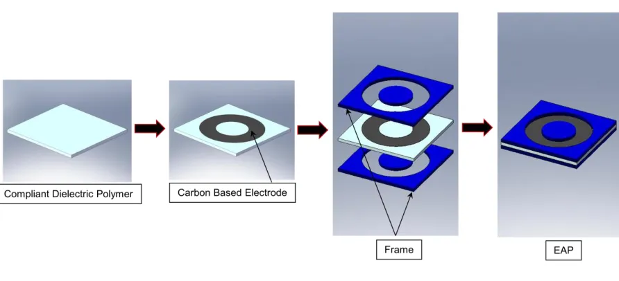
The Dielectric Electro-Active Polymer actuator considered in this study has a circular

geometry. It is constructed with a film of silicone material and pasted with carbon based

electrodes held together in place by a plastic frame. Figure 5 shows the schematic for the

DEAP construction process.

Figure 5: DEAP actuator

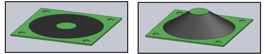
The DEAP actuator has a circular geometry as can be seen in Figure 6 . This particular

15

solid frame adhered to a proprietary pre-strained silicone based elastomer film. They are

approx. 1 inch2 in size, and the elastomer layer is a few 10‘s of µm thick in the absence of

any load.

Figure 6: Electroactive Polymer Actuator Geometry. Solidworks model [33].

Two black carbon-based electrodes make up the effective DEAP area. The thickness of the

carbon electrodes is assumed to be 10 µm. This makes the DEAP actuator a layered

composite structure with electrode-elastomer-electrode. The circular mounting section made

from the frame material is also adhered at the center of the actuator. When the actuator is

loaded at its center mechanically or a potential difference is applied across its electrodes, it

exhibits out-of-plane motion by displacing the center mount, as shown in Figure 6 (right).

The pasted electrodes have an effect on the mechanical response of the DEAP actuator and

hence they have to be accounted for in the model in order to capture their effect.

3.2 Boundary Conditions

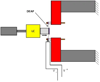
Generally, the DEAP actuator is mechanically pre-loaded and then an electric potential

applied across its electrodes. This helps to use the stroke caused by the electrostriction as a

displacement stroke. The actuator geometry considered in this study has a center mount, as

discussed in the earlier section, which can be used to apply a mechanical force to pre-load the

16

attached to a load cell (LC) can be used to illustrate this further as shown in Figure 7.

Figure 7: Pre-loading the DEAP in out-of-plane direction schematic. [33]

The above situation can be shown in a simplified diagram as sketched in Figure 8.

17

The circular geometry of the DEAP actuator and uniform thickness all over also makes it

symmetric about an axis perpendicular to the DEAP surface through the center. Thus, axial

symmetry can be used while modeling the geometry using COMSOL. This helps in

converting a three dimensional problem into a simplified two dimensional axially symmetric

one. Another advantage of this simplification is that the problem becomes computationally

more efficient.

The commercially available finite element software COMSOL Multiphysics [28] has been

used to develop a finite element model. COMSOL Multiphysics is a powerful interactive

environment for modeling and solving a variety of engineering and physics problems based

on partial differential equations (PDEs). There are several application modes, based upon

basic physics (structural, electrical, fluids etc) which can be used to model problems

involving single physics or more than one of the application modes can be used in

conjunction with others to model coupled field problems.

For modeling the electro-mechanically coupled DEAP actuator, three COMSOL Multiphysics‘ environments are used – Structural mechanics, Electrostatics and Deformed

Mesh. The Structural Mechanics module is used to model the response of the DEAP

undergoing mechanical loading. The Electrostatics module is used to apply input voltage and it also generates the Maxwell‘s Stress Tensor along the boundaries of the electrodes. The

deformed mesh module allows the electrostatic boundary conditions to be applied even

though the boundaries of the computational domain move due to the applied structural

boundary conditions. The technique for mesh movement is called an arbitrary

Lagrangian-Eulerian (ALE) method. In the special case of a Lagrangian method, the mesh movement

follows the movement of the physical material. Lagrangian method is often used in solid

mechanics, where the displacements often are relatively small.

When the material motion is more complicated, like in a fluid flow model, the Lagrangian

method is not appropriate. For such models, an Eulerian method, where the mesh is fixed, is

18

The ALE method is an intermediate between the Lagrangian and Eulerian methods, and it

combines the best features of both—it allows moving boundaries without the need for the

mesh movement to follow the material.

3.2.1 Mechanical Boundary Conditions

The simplification of geometry for analysis enables to model the geometry as a simple strip

with the width equal to the thickness of the elastomer and similar strips for the electrodes

above and below the elastomer strip. The modeled geometry is thus only a three strip

composite. Since, the outer plastic frame is rigid as compared to the elastomer, the outer end

of the elastomer can be considered fixed to a rigid frame. Similarly, the circular part of the

frame at the center of the DEAP (the center mount) is rigid as compared with the elastomer

material and hence no radial displacement of the polymer occurs at the inner end. All these

mechanical boundary conditions are illustrated in Figure 9

Figure 9: Mechanical Boundary Conditions

The right end of the DEAP geometry is specified as the fixed end. The left end has a roller

boundary condition which restricts its movement in the radial direction. The displacement or

force boundary condition is also applied on the left boundary of the elastomer 2D geometry,

thus allowing simulations in both force control mode and displacement control mode. The

force boundary condition is used when simulating a pre-deflected DEAP to produce stroke

19

3.2.2 Electrical Boundary Conditions

The electrical boundary conditions are basically the voltage boundary conditions on the

electrodes. Voltage is specified as a boundary condition on the top electrode. The boundaries

of the upper electrode are specified as port and the port can be used to specify input. ‗Ground‘ is used as a boundary condition on the boundaries of the bottom electrode. The

Figure 10 below shows the electrical boundary conditions.

Figure 10: Electrical Boundary conditions

3.2.3 Electromechanical Boundary condition

The Electroactive Polymer actuator system is a coupled electro-mechanical system. Hence,

there should be a way to couple the electrostatics with the structural deformation in the finite

element model. The Electrostatics physics environment in COMSOL Multiphysics allows the

generation of a Maxwell Stress tensor. The Maxwell force can be extracted from this stress

tensor is available with units of Newton per unit area to be applied as a boundary condition.

A force variable is created on the electrode sub-domains to generate a Maxwell stress tensor.

The Maxwell force is then applied as a force boundary condition on the upper and the lower

electrodes using the structural mechanics subdomain, thus coupling the two physics.

Another way to couple the two physics is by using the Pelrine‘s equation as described in the

Section 2.4.2. The equation for pressure as derived by Pelrine et al is applied as a boundary

condition on the upper and lower electrodes using the structural mechanics module in

20

3.3 Finite Element Mesh

The elastomer and the electrode geometry is regular and it is easier to mesh them using a

mapped mesh and quad elements. The elements have a quadratic shape function. The

elements on the boundary are specified before meshing the geometry. The boundary

discretization can be done in a couple of ways. The elements along the horizontal can be of

uniform sizes which will make a uniform mesh in the sub-domain, or their size can vary

depending on the size of the elements on the vertical boundary. So the elements near the

vertical boundaries get smaller and their sizes are the same as that on the vertical edges. This

creates high quality elements (with an aspect ratio close to 1) near the edges which help in

dealing with singularities occurring at the edges due to mechanical boundary conditions.

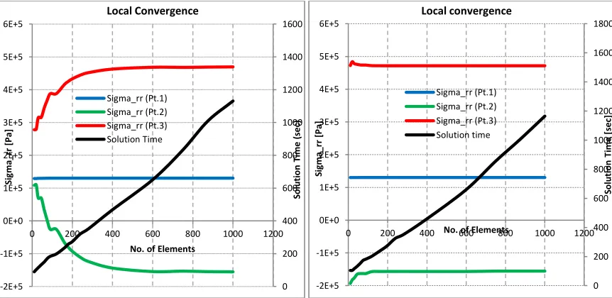
Both of the above mentioned meshing options were evaluated by running mesh convergence

tests by varying the number of elements and deciding the type of mesh and the optimum

number of elements in that mesh. Local quantity stress at important locations as shown in

Figure 11 and global quantity maximum displacement were used as convergence criteria.

21

Figure 12: Global mesh convergence with uniform mesh (left) and non-uniform mesh (right).

Figure 13: Local mesh convergence with uniform mesh (left) and non-uniform mesh (right).

From Figure 12 and Figure 13 it is quite clear that the rate of convergence when using a

non-uniform mesh (smaller elements near the ends and coarse mesh towards the center of the

elastomer strip) is much higher than that with uniform size elements throughout the sub-

0 200 400 600 800 1000 1200 -1.25E-3 -1.25E-3 -1.24E-3 -1.24E-3 -1.23E-3 -1.23E-3 -1.22E-3

0 200 400 600 800 1000 1200

So lut io n ti me (s e c) Z-di sp la ce me nt [m]

No. of Elements

Global Mesh Convergence

Z-displacement [m] Time 0 200 400 600 800 1000 1200 -1.25E-3 -1.25E-3 -1.25E-3 -1.25E-3 -1.25E-3 -1.25E-3 -1.24E-3 -1.24E-3

0 200 400 600 800 1000 1200

So lut io n Ti me [sec ] Z-D isp la ce me nt [m]

No. of Elements

Global Mesh Convergence

Z-Displacement [m] Time 0 200 400 600 800 1000 1200 1400 1600 -2E+5 -1E+5 0E+0 1E+5 2E+5 3E+5 4E+5 5E+5 6E+5

0 200 400 600 800 1000 1200

Solution T ime (se c) Si gma _r r [P a]

No. of Elements

Local Convergence Sigma_rr (Pt.1) Sigma_rr (Pt.2) Sigma_rr (Pt.3) Solution Time 0 200 400 600 800 1000 1200 1400 1600 1800 -2E+5 -1E+5 0E+0 1E+5 2E+5 3E+5 4E+5 5E+5 6E+5

0 200 400 600 800 1000 1200

Solution T ime [sec] Si gma _r r [P a]

No. of Elements

Local convergence

22

domain. Hence, a non-uniform mapped mesh is chosen for the elastomer sub-domain. The

elastomer has four divisions vertically and sixty divisions horizontally giving a total of 240

elements. The elastomer has a single layer of mapped meshed quad elements with a quadratic

shape function. The electrostatics module also requires air to be modeled as a surrounding

medium around the DEAP. The air is meshed with a free triangular mesh. The mesh for the

entire geometry is as seen in Figure 14.

23

Chapter 4. MECHANICAL SIMULATIONS

The commercial Finite Element software COMSOL is used to simulate the DEAP actuator.

This chapter describes the simulation procedure for the mechanical characterization of the

actuator material in COMSOL. This includes not only the elastomer but also the electrode

material. It also describes the experiments used to compare the simulation results with the

experimental data. A systematic approach to vary the material parameters is also discussed.

Global results in the form of force-displacement plots are presented. Contour plots for

stresses at specific local points on the elastomer and electrodes are also shown

4.1 Experiments

This section presents the experimental procedure and tests that are compared to the

simulation results for validation. Out of plane deformation experiments have been performed

on actuators. A simple tensile test on a small strip of elastomer material is done. The

elastomer is clamped at both the ends. A picture of the set-up is shown in Figure 15where

one of the ends is held fixed and the other end is pulled on with the help of a linear actuator.

A load cell is used with the actuator to note the reaction force and a force-displacement graph

is plotted. Using the geometry of the elastomer sample a stress-strain curve is plotted as

shown in Figure 16. A linear approximation of the stress-strain curve gives the approximate

Young‘s modulus of the elastomer material. This Young‘s modulus serves as the initial

approximation for simulations of the actuator.

24

Figure 16: Stress vs Strain plot for simple tensile experiment on the elastomer.

In the experiments on the actuator, the actuator is deformed to a fixed out-of-plane

displacement using a mechanical actuator and the force is measured with a load cell. A

schematic of the out-of-plane deformation experiments is shown in Figure 17. The

displacement is measured from the rest position of the elastomer. The experiments are

conducted on actuator samples without coated electrodes and samples with electrodes coated

on them. This helps to characterize the elastomer separately. The electrodes can then be

included into the model and a systematic parameter variation can be done to arrive at the

correct material parameters. The details of the experimental procedure can be found in [32].

Figure 17: Schematic for out-of-plane deformation experiments [33].

y = 1E+06x - 67654

0E+00 2E+05 4E+05 6E+05 8E+05 1E+06 1E+06 1E+06

0 0.1 0.2 0.3 0.4 0.5 0.6 0.7 0.8

Str

e

ss [Pa]

Strain

Stress Vs Strain

25

4.2 Simulations

As mentioned in the earlier section, the out-of-plane deformation experiments are done on

actuator samples without coated electrodes and experimental conditions are simulated in

COMSOL. The structural mechanics module is chosen in order to simulate response of the

elastomer to purely mechanical loading. The experiments for mechanical characterization are

as mentioned in the section 4.1. The structural mechanics offers choice of several material

models to choose from to apply to specify the material type. Hyperelastic material models are

chosen to model the elastomer. Hyperelastic materials further allow the use of three types of

material models - The Neo-Hookean, Mooney-Rivlin or the Murnaghan material model. In

this work, the Neo-Hookean and Mooney-Rivlin material models have been used to model

the elastomer and the electrodes. The Murnaghan model is generally used for non-linear

acoustoelasticity and not considered in this study. COMSOL Multiphysics also supports

geometric non-linearity (or non-linear geometry as is sometimes called) through the option of

Large deformation ON/OFF. This option is kept for ON all the simulations.

4.2.1 Pre-strain

COMSOL Multiphysics does not support the inclusion of a pre-strain or a pre-stress when

using hyperelastic material models. This warrants the use of a stationary analysis prior to the

actual analysis in-order to include the required pre-strain in the material. A stationary

analysis would require modeling the geometry prior to any pre-strain. It would include the

following steps:

1. Modeling the un-strained geometry

2. Running a stationary analysis which would include a required pre-strain in

appropriate directions (in-plane and the thickness directions). Saving this solution.

3. Running the actual analysis starting from the saved solution is step 2 with

experimental boundary conditions.

26

pre-strained. So, the equations defined for the elastomer sub-domain are modified to include

the appropriate amount of pre-strain. In COMSOL, for hyperelastic materials, the stresses

and strains are calculated from the Strain energy function which is defined using the

components of the deformation tensor F. The deformation tensor is made up of displacement

components and their derivatives. A stationary analysis is used to extract the values of the

derivatives of the displacements for their values in the pre-strained state. These values are

added to the equations defining the elastomer in the physics equations of the structural

analysis module.

4.2.2 Solver

In COMSOL Multiphysics a number of solvers can be used to solve the PDEs. Their memory

requirements and computation times vary over a wide range and so does their capability of

solving problems having range of degrees of freedom. For the problem of the

electromechanical coupling of DEAP the number of degrees of freedom to solve for are in

the range of 2000 – 2500. The SPOOLS solver is a good option for solving such a problem. It

also uses a lot less memory (~ 1GB) than some of the other solvers and gives the solution in

an acceptable amount of time (~ 200 – 300 sec).

A parametric variation is specified for the input by using a parameter which uniformly varies

the input from zero to the maximum specified value. This helps with gradual loading of the

actuator and helps in convergence whereas applying the input (displacement or force) in one

step sometimes leads to convergence problems.

4.2.3 Results

The mechanical simulations help to arrive at the correct material parameters, both, for the

elastomer and the electrodes. The elastomer is characterized by using fixed displacement

simulations and comparing the results in the form of force vs. displacement plots to those

obtained from experiments. The variation of material parameters is done as mentioned

27

1. The initial parameters used are based upon the approximate Young‘s modulus

obtained from the stress-strain diagram of the tensile experiment. This modulus, as

shown in Figure 16, is 1 MPa.

2. A force displacement plot obtained from the simulation is compared with the

experimental force displacement plot.

3. The material parameters for the elastomer are varied by varying the Young‘s

modulus.

4. The material parameters for each of the hyperelastic model Neo-Hookean &

Mooney-Rivlin are finalized based on the fit between the experimental and simulation curves.

The Neo-Hookean material model in COMSOL requires the material parameters shear modulus G and bulk modulus κ and the Mooney-Rivlin material model requires the material

parameters C10 and C01. These parameters are derived using the equations presented in

Section 2.3.3. The values of the parameters derived for the two material models are as shown

in Table 1.

Table 1: Material parameters for the two material models

Young's Modulus

Neo-Hookean Material Parameters Mooney Rivlin Material Parameters G [Pa] κ [Pa] C10 [Pa] C01[Pa]

1 MPa 3.34 x 105 16.67 x 106 2.5 x 105 -0.83 x 105

1.25 MPa 4.16 x 105 20.83 x 106 3.1235 x 105 -1.04 x 105

1.5 MPa 5 x 105 25 x 106 3.75 x 105 -1.25 x 105

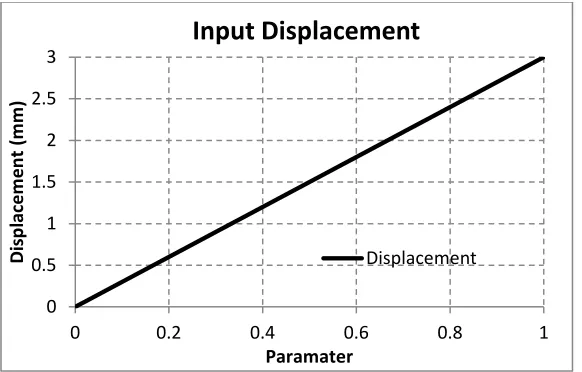
The simulations are run in displacement control mode. The displacement is the input and is

slowly ramped from zero to 3 mm in the out-of-plane direction. The plot of input

28

Figure 18: Displacement Input in displacement control simulation.

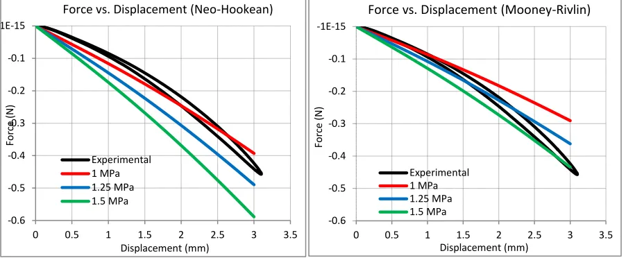
The reaction force is plotted against the displacement as shown in Figure 19. As seen from the plots, the stiffness of the elastomer increases for a small change in the Young‘s modulus value. It can be seen that the simulation results for elastomer Young‘s modulus values of

1.25 MPa with Mooney-Rivlin material model and 1 MPa in case of Neo-Hookean material

model fit the experimental data well and represent the average experimental response. The

other curves are either too stiff of less stiff as compared to the experimental result. So, for

further simulations we use the data corresponding to these two values of Young‘s modulus

and the respective material models.

0 0.5 1 1.5 2 2.5 3

0 0.2 0.4 0.6 0.8 1

D

isp

lac

e

m

e

n

t

(m

m

)

Paramater

Input Displacement

29

Figure 19: Force vs Displacement curves for different values of elastomer Young's modulus. [34]

A similar modeling approach is used to model the electrode material. Each electrode is

assumed to be a homogenous and continuous body and they are also modeled using

Hyperelastic material models. The electrodes are modeled connected to the elastomer

geometry and exactly similar procedure is followed as mentioned for the elastomer parameter

variation. The values of material constants for the various Young‘s moduli values used for

electrodes are as shown in Table 2. The materials constants for Mooney-Rivlin material are derived exactly as derived for the elastomer model.

Table 2: Material parameters for different values of young's modulus and material model

Young's Modulus

Neo-Hookean Material Parameters Mooney Rivlin Material Parameters G [Pa] κ [Pa] C10 [Pa] C01[Pa]

2 MPa 6.67 x 105 33 x 106 4.9 x 105 -1.67 x 105

2.5 MPa 8.33 x 105 41.67 x 106 6.25 x 105 -2.08 x 105

3 MPa 1 x 106 50 x 106 7.5 x 105 -2.5 x 105

Figure 20 shows the force vs. displacement curves for elastomer with electrodes. From the -0.6 -0.5 -0.4 -0.3 -0.2 -0.1 -1E-15

0 0.5 1 1.5 2 2.5 3 3.5

Fo rc e ( N ) Displacement (mm)

Force vs. Displacement (Neo-Hookean)

Experimental 1 MPa 1.25 MPa 1.5 MPa -0.6 -0.5 -0.4 -0.3 -0.2 -0.1 -1E-15

0 0.5 1 1.5 2 2.5 3 3.5

Fo rc e ( N ) Displacement (mm)

Force vs. Displacement (Mooney-Rivlin)

30

experimental data, it can be seen that the DEAP exhibits a highly hysteretic behavior. The

plot for Mooney-Rivlin material with electrode Young‘s modulus equal to 2 MPa and

Neo-Hookean model with electrode modulus equal to 3 MPa are approximately in the center of

the hysteresis loop. Depending upon the frequency with which the experiments are

conducted, the force can vary between the two branches of the hysteresis loop for a given

displacement of the actuator. The material parameters used for the simulation are chosen to

represent the average values. The force-displacement curve for 2 MPa Mooney-Rivlin model

and 3 MPa Neo-Hookean model (as seen in Figure 20) pass approximately through the center

of the hysteresis loop and the corresponding material parameters are chosen for simulating

the electrodes. There is a clear difference between the force-displacement curves for the

elastomer without electrodes and the elastomer with electrodes. Hence, in order to simulate

the DEAP system, the effects of electrodes on the material behavior need to be taken into

account.

Figure 20: Force vs Displacement for different values of electrode Young's modulus. [34]

The hyper-elastic material models used are able to account for the non-linear material

behavior of the elastomer and the electrodes. Also, modeling the DEAP actuator as a

composite geometry with elastomer and electrode layers enables to account for the difference -0.8 -0.7 -0.6 -0.5 -0.4 -0.3 -0.2 -0.1 0

0 0.5 1 1.5 2 2.5 3 3.5

For

ce

(N)

Displacement (mm)

Force vs. Displacement (with Electrodes)

Neo-Hookean model Experimental 1.5 Mpa 2 MPa 3 MPa -0.8 -0.7 -0.6 -0.5 -0.4 -0.3 -0.2 -0.1 0

0 0.5 1 1.5 2 2.5 3 3.5

Force

(N)

Displacement (mm)

Force vs. Displacement (with Electrodes) Mooney-Rivlin model

31

in mechanical response from that of the elastomer. An approximation for the material

properties of the elastomer and the electrodes is also made possible by variation of the

material parameters in a systematic way and comparing the simulation results to the

experimental results. This also sets up the model to be used with electro-mechanical

boundary conditions to simulate the electro-mechanical coupling which is discussed in the

32

Chapter 5. ELECTRO-MECHANICAL

COUPLING

The actuation of the DEAP actuator is a result of an electro-mechanical phenomenon where

mechanical displacement of the DEAP is caused due to electrostriction when a voltage is

applied across the electrodes. This chapter describes the simulations which account for the

electromechanical coupling. The simulations are performed for both displacement control

and force control and the results are presented.

5.1 Experiments

There are modes of experiments that are performed on the DEAP actuators – The

displacement control mode and the force control mode. In the displacement control mode the

DEAP actuator is displaced to certain known displacement value and then the voltage is

applied across the electrodes by keeping the displacement fixed. The experimental setup for

this experiment is similar to that as mentioned for the out-of-plane deformation experiments.

A linear actuator is used to displace the DEAP to the specified displacement and voltage is

cycled from zero to 2500 V and back to zero. The schematic for the experiments is as shown

in Figure 21.

33

For force control experiments different masses are suspended from the center of the DEAP

and the voltage is again cycled from zero to 2500V and back to zero. The displacement of the

center of the DEAP is recorded using a laser sensor. The stroke of the DEAP is calculated

using the deflection values at the start of the voltage actuation and the maximum deflection

of the DEAP. The schematic and the actual setup for the suspended weight experiments are

as shown in Figure 22.

Figure 22: Schematic of test setup (left) and the actual set-up (right). [34]

5.2 Simulation Procedure

The electromechanical simulation is run according to the following procedure:

1. The mechanical force/displacement is first applied from zero to its maximum value

without applying any input voltage.

2. When the force reaches its maximum value it is held constant at that value.

3. The input voltage is cycled from zero to 2.5 kV and back to zero keeping the applied

34

5.3 Results

5.3.1 Time Resolved Data

The procedure for the electromechanical simulations has been mentioned in Section 5.2. A

graphical representation of the inputs is as shown in Figure 23 (left). The time resolved

displacement data for the above input is as shown in Figure 23 (right). As it can be seen from

the output plot, the displacement increases as the applied force is increased to the maximum

pre-deflection value. The vertical displacement further increases as the input voltage are

applied holding the force constant at its maximum value. This further increase in

displacement is the stroke of the actuator.

Figure 23: Time resolved data. Input parameters (top left), Displacement output (top right). Experimental

displacement output for one voltage cycle (bottom). [34]

0 500 1000 1500 2000 2500 3000 0 0.05 0.1 0.15 0.2 0.25 0.3 0.35 0.4

0 10 20 30 40

Vo lt ag e (V) Fo rc e ( N )

Time / Parameter

Force Voltage -3.5 -3 -2.5 -2 -1.5 -1 -0.5 0

0 10 20 30 40

Di sp lac eme n t (mm)

Time / Parameter

35

A similar plot can be made when the simulations are run in displacement control mode. In

this case displacement is the input and the reaction force becomes the output. The reaction

force is measured at the inner vertical boundary of the elastomer. The time resolved data for

simulations in displacement control mode is as shown in Figure 24.

Figure 24: Time resolved data for Displacement control (Simulation – Top, Experimental – Bottom).

5.3.2 Local Results

5.3.2.1 Deformation and Stress

The Figure 25 shows the series of deformed shapes for the elastomer during its mechanical

deflection and electrical actuation. The deformation is similar to a beam bending deflection.

The curved bending shows that the deformation is representative of a three dimensional

deformation. 0 500 1000 1500 2000 2500 3000 0 0.5 1 1.5 2 2.5

-5 5 15 25 35

V ol tage [ V ] D is pl acem e nt [ m m ]

Time / Parameter

Input Parameters Displacement Voltage -0.4 -0.35 -0.3 -0.25 -0.2 -0.15 -0.1 -0.05 0

0 10 20 30 40

Force

[

N]

Time / Parameter

Force vs Time (simulation)

Force 0 500 1000 1500 2000 2500 3000

10 15 20 25 30

Force

(N)

Voltage (V)

Voltage vs. Time (Experiment)

-0.3 -0.25 -0.2 -0.15 -0.1 -0.05 0

0 10 20 30 40

Force

(N)

Time

36

Figure 25: Deformation shapes of the elastomer during pre-deflection and actuation. [34]

A closer view at the stresses and the deformation at the ends of the elastomer and the

electrodes are shown in Figure 26 and Figure 27. Figure 26 shows the Second-Piola Kirchoff

stress in the radial direction while Figure 27 shows the Second-Piola Kirchoff stresses in the

thickness directions. The radial stresses are higher at both the ends of the elastomer because

of the slight bending occurring due to the boundary conditions. The stresses in the elastomer

away from the ends are fairly uniform and they reduce slightly as we move from the inner

end to the outer end due to the slightly increasing radial area of the elastomer. The stresses

in the electrodes show similar variation as those in the elastomer. They are lower because the

electrodes are not pre-strained initially.

In the case of the stresses in the thickness directions the plots show stresses during maximum

actuation voltage. The pressure on the elastomer in the thickness direction is the maximum at

the max actuation voltage and so are the compressive stresses. At the ends of the elastomer

37

thickness in the electrodes are constant and equal to zero.

38

39 5.3.2.2 Electric Field

The contour plots for the electric field are as shown in Figure 28. The electric field in the

elastomer is very high and is of the order of 108 V/m. The upper electrode has positive charge

and the lower electrode has a negative charge. Hence, the direction of the electric field is

from the upper electrode to the bottom electrode. Also the value of the electric field in the

electrodes is zero as expected.

40 5.3.2.3 Charge Distribution

The charge distributions on the internal surfaces of the electrodes are plotted against the

length of the electrode and shown in Figure 29. The charges on the upper and the lower

electrode are have same magnitude but opposite in sign. There are singularities at the ends of

the electrode which can be seen in the plots. The surface charge density on the rest of the

electrode is almost constant at C/m2.

Figure 29: Surface Charge densities on the internal surface of the top electrode (left) and bottom electrode (right).

5.3.3 DEAP Stroke

The design of DEAP actuator in a pumping system would depend upon the requirements of

the flow rate and pressure head. An appropriate amount of DEAP stroke would be required to

achieve these and hence the stroke prediction is necessary for and effective design.

Experiments are done for stroke estimation as per the following procedure. Different masses

are suspended from the center of the elastomer and then the voltage is cycled from zero to 2.5

kV and back to zero. The pre-deflection due to the suspended weights as well as the

maximum displacement after cycling the voltage are noted. The difference between

maximum displacement and the pre-deflection gives the stroke of the actuator for the weight 0.002

0.0025 0.003 0.0035 0.004

-0.0005 0.0015 0.0035

Sur fa ce C ha rg e D ens ity [C /m2 ]

Electrode Length [m]

Surface Charge Density (Top Electrode) -0.004 -0.0035 -0.003 -0.0025 -0.002

-0.0005 0.0005 0.0015 0.0025 0.0035 0.0045

Sur fa ce C harg e D e ns it y [C /m 2]

Electrode Length [m]

41

suspended and the corresponding pre-deflection. A schematic of the experimental setup is as

shown in Figure 30.

Figure 30: Test setup schematic (left) and actual picture of the test (right). [34]

The results presented are using the Mooney-Rivlin and the Neo-Hookean material models with material parameters corresponding to the electrode Young‘s modulus of 2 MPa and 3

MPa respectively. As shown in Figure 31, the value of the suspended mass is plotted against

the corresponding stroke of the DEAP. As the weight suspended is increased, the elastomer

gets stiffer, due to larger pre-deflections and the stroke decreases. The simulation results also

show this trend of decreasing stroke similar to the experimental results. The experimental

curve will shift towards the right if the DEAP is loaded quasi-statically thus giving it time to

42

Figure 31: Suspended Mass vs Stroke.

5.3.4 Global Results

5.3.4.1 Force-Voltage Characteristics

A graph of Force vs. Voltage has been plotted (Figure 32) for simulations run with fixed

displacement of the elastomer and with Mooney Rivlin and Neo Hookean material models.

The displacement is held constant at 2 mm. The force has been normalized prior to plotting.

As seen from the experimental force displacement plots of Figure 3, the DEAP shows a

hysteretic behavior. So, for a displacement of 2mm, the corresponding force can vary

anywhere between the two branches of the hysteresis loop, depending on the creep of the

material. Also, the model currently does not include the viscoelastic behavior. Hence, for

comparison, we normalize the force from the experiments and the simulations and plot it

against the voltage. It can be seen that the amplitude of the force from simulations shows a

good match to the experimental value. 0

5 10 15 20 25 30

0 0.1 0.2 0.3 0.4 0.5 0.6

M

ass

(g

ram

s)

Stroke (mm)

Mass - Stroke

43

Figure 32: Blocking Force vs Voltage curve for fixed displacement of 2mm.

5.3.4.2 Capacitance Variation (Sensing Applications)

The capacitance of the DEAP varies as the actuator get deformed out-of-plane. The

capacitance is given by the equation:

0 r

A C

d

 

  

(37)

where C is the capacitance, ε0 and εr are the permittivity of free space and the dielectric

constant of the elastomer, A is the surface area of the elastomer and d is the elastomer

thickness.

As the elastomer gets deformed the area will increase and the thickness decreases. Hence, the

capacitance of the DEAP is a function of the deformation field. This can be potentially

utilized to use the DEAP in a dual actuation and sensing mode. 0

0.02 0.04 0.06 0.08 0.1 0.12 0.14

0 500 1000 1500 2000 2500

Force

(N)

Voltage (V)

Force vs. Voltage