Effect of cyclic loading on the mechanical behaviour of structural steels at various temperatures

University of Windsor University of Windsor

Scholarship at UWindsor

Scholarship at UWindsor

Electronic Theses and Dissertations Theses, Dissertations, and Major Papers

2012

Effect of cyclic loading on the mechanical behaviour of structural

Effect of cyclic loading on the mechanical behaviour of structural

steels at various temperatures

steels at various temperatures

University of Windsor

Follow this and additional works at: https://scholar.uwindsor.ca/etd

Recommended Citation Recommended Citation

Hamdoon, Muhsin M., "Effect of cyclic loading on the mechanical behaviour of structural steels at various temperatures" (2012). Electronic Theses and Dissertations. 4812.

https://scholar.uwindsor.ca/etd/4812

This online database contains the full-text of PhD dissertations and Masters’ theses of University of Windsor students from 1954 forward. These documents are made available for personal study and research purposes only, in accordance with the Canadian Copyright Act and the Creative Commons license—CC BY-NC-ND (Attribution, Non-Commercial, No Derivative Works). Under this license, works must always be attributed to the copyright holder (original author), cannot be used for any commercial purposes, and may not be altered. Any other use would require the permission of the copyright holder. Students may inquire about withdrawing their dissertation and/or thesis from this database. For additional inquiries, please contact the repository administrator via email

EFFECT OF CYCLIC LOADING ON THE MECHANICAL BEHAVIOUR

OF STRUCTURAL STEELS AT VARIOUS TEMPERATURES

by

MUHSIN M. HAMDOON

A Dissertation

Submitted to the Faculty of Graduate Studies

Through the Department of Mechanical, Automotive and Materials Engineering in Partial Fulfillment of the Requirements for

the Degree of Doctor of Philosophy at the University of Windsor

Windsor, Ontario, Canada 2012

Effect of Cyclic Loading on the Mechanical Behaviour of Structural Steels

at Various Temperatures

by

MUHSIN M. HAMDOON

APPROVED BY:

_________________________ S. Das, External Examiner University of Detroit Mercy

______________________________________________ V. Stoilov

Department of Mechanical, Automotive and Materials Engineering __________________________________________

A. Fartaj

Department of Mechanical, Automotive and Materials Engineering ______________________________________________

D. Green

Department of Mechanical, Automotive and Materials Engineering ______________________________________________

N. Zamani, Advisor

Department of Mechanical, Automotive and Materials Engineering ______________________________________________

S. Das, Co-advisor

Department of Civil and Environmental Engineering ______________________________________________

R. Nakhaie, Chair of Defense Department of Sociology

DECLARATION OF CO-AUTHORSHIP/PREVIOUS PUBLICATION

I. Co-Authorship Declaration

I hereby declare that this dissertation incorporates the outcome of a joint research undertaken in collaboration with Dr Sreekanta Das, Dr Nader Zamani, and Daniel Grenier under the supervision of both Dr S. Das and Dr N. Zamani. The collaboration is covered in Chapters 3 and 4 of the dissertation. In all cases, the key ideas, primary contributions, experimental designs, data analysis and interpretation, were performed by the author, and the contribution of co-authors.

Dissertation

Chapter Publication title/full citation Publication status

Chapters 3

and 4 Experimental study on the effect of strain cycles on mechanical properties of AISI 1022 steel published Chapters 3

and 4 Effect of cyclic strain on mechanical behaviour of structural steels in room and low temperatures submitted

I am aware of the University of Windsor Senate Policy on Authorship and I certify that I have properly acknowledged the contribution of other researchers to my dissertation, and have obtained written permission from each of the co-author(s) to include the above material(s) in my dissertation.

I certify that, with the above qualification, this dissertation, and the research to which it refers, is the product of my own work.

II. Declaration of Previous Publication

This dissertation includes two original papers that have been previously published or submitted for publication in peer reviewed journals.

I declare that, to the best of my knowledge, my dissertation does not infringe upon anyone’s copyright nor violate any proprietary rights and that any ideas, techniques, quotations, or any other material from the work of other people included in my dissertation, published or otherwise, are fully acknowledged in accordance with the standard referencing practices. Furthermore, to the extent that I have included copyrighted material that surpasses the bounds of fair dealing within the meaning of the Canada Copyright Act, I certify that I have obtained a written permission from the copyright owners to include such materials in my dissertation.

ABSTRACT

It was found that the cyclic loading has a considerable effect on the mechanical behaviour of materials. This effect may lead to an early failure which results in human and economical losses. This study was developed to investigate changes in mechanical behaviour of structural steels. Two steels were considered and these are: G40.21 350WT which is used in ship hull structures and AISI 1022 HR which is used in general structural applications. The study was carried out in three parts: experimental, statistical, and numerical. The experimental tests were conducted using strain-controlled axial loading in room, zero, and sub-zero temperatures. In the statistical part, empirical formulae were derived to predict changes in mechanical properties as well as assessment of the experimental strain-life relationship. In the numerical part, a numerical model was developed to determine the strain-life relationship.

DEDICATION DEDICATION DEDICATION DEDICATION

To the memory of my father and mother;

To my siblings, wife, and children (Abdulrahman, Luqman, and Issra);

ACKNOWLEDGEMENTS

This study was carried out under the supervision and guidance of Dr. Sreekanta Das and Dr. Nader Zamani to whom I am profoundly grateful for their kindness, endless constructive commentaries, valuable suggestions, and continuous support and encouragement throughout my study. They devoted their time and sincere efforts to provide all necessary research facilities for this work.

I would like to express my appreciation to all the committee members: Dr. Shuvra Das, Dr. Vesselin Stoilov, Dr. Daniel Green, and Dr. Amir Fartaj for their constructive suggestions to improve this dissertation.

The acknowledgement also goes to all technical staff; especially, Matthew St. Louis, Patrick Seguin and Lucian Pop for their continuous assistance in laboratory work.

Furthermore, I am grateful to Dan Edelstein for his assistance in statistical analysis, to Patrick Kiely for his assistance in troubleshooting the MTS control system, and to Elizabeth Munn for her review of the English language in this dissertation.

TABLE OF CONTENTS

DECLARATION OF CO-AUTHORSHIP/PREVIOUS PUBLICATION ... iii

ABSTRACT ... v

DEDICATION ... vii

ACKNOWLEDGEMENTS ... vii

LIST OF TABLES ... xiv

LIST OF FIGURES ... xvi

LIST OF APPENDICES ... xxiv

CHAPTER 1 INTRODUCTION ... 1

1.1 SCOPE OF THE WORK ... 1

1.2 OBJECTIVES OF THE STUDY... 2

1.3 PREVIOUS STIDIES ... 2

1.4 METHODOLOGY ... 3

2 LITERATURE REVIEW ... 4

2.1 MATERIAL RESPONSE ... 4

2.1.1 Crystallography ... 4

2.1.1.1 Atomism ... 4

2.1.1.2 Crystallite... 5

2.1.2 Crystallographic Defects ... 6

2.1.2.1 Point Defects ... 6

2.1.2.2 Line Defects ... 8

2.1.2.4 Bulk Defects ... 13

2.1.3 Deformation ... 13

2.1.3.1 Elastic Deformation ... 13

2.1.3.2 Plastic Deformation ... 14

2.1.3.3 Dislocation Theory of Slippage ... 18

2.1.3.4 Stress-strain Curve: Ductile Materials ... 20

2.1.3.5 Stress-strain Curve: Brittle Materials ... 22

2.1.3.6 Cyclic Stress-strain Curves ... 23

2.1.4 Cycle-dependent Material Response ... 25

2.1.4.1 Cyclic Stress-strain Response ... 25

2.1.4.2 Stress-controlled Test ... 26

2.1.4.3 Strain-controlled Test ... 27

2.2 FATIGUE CONCEPT ... 29

2.2.1 Crack Initiation ... 29

2.2.2 Crack Propagation ... 33

2.2.3 Fracture Behaviour ... 39

2.2.3.1 Toughness ... 39

2.2.4 Fatigue Damage with Mean Values ... 41

2.2.4.1 Cyclic Ratcheting ... 41

2.2.4.2 Mean-stress Relaxation ... 43

2.2.5 Cycle-dependent Changes in Mechanical Properties-Previous Studies .. 43

2.3 FATIGUE LIFE PREDICTION ... 45

2.3.1 Linear Damage Rule ... 45

2.3.2 Nonlinear Damage Theories ... 45

2.3.3 Strain-life Theories ... 46

2.3.3.1 Existing Methods for Estimation of Strain-life Fatigue Parameters... 49

2.4 ENVIRONMEENTAL EFFECT ... 51

2.4.1 Low-temperature Effect... 51

2.4.1.1 Monotonic Behaviour at Low Temperatures ... 51

2.4.1.2 Stress-Life (S-N) Behaviour ... 52

2.4.1.3 Strain-Life (ε-N) Behaviour ... 54

2.4.1.4 Fatigue Crack Growth (da/dn-∆k) Behaviour ... 56

3.1 MATERIALS SELECTION ... 60

3.1.1 Offshore Applications ... 60

3.1.2 American Bureau of Shipping (ABS) ... 62

3.1.2.1 Ordinary-Strength Hull Structural Steel ... 62

3.1.2.2 Higher-Strength Hull Structural Steel ... 62

3.1.2.3 Low Temperature Materials ... 63

3.1.3 American Society for Testing and Materials ... 63

3.1.4 Canadian Standards Association (CSA) ... 63

3.1.5 Advanced Materials and Process Tech. Info. Analysis Centre ... 63

3.1.6 Det Norske Veritas (DNV) ... 65

3.1.7 Steels Chosen ... 65

3.2 TEST PROCEDURE ... 67

3.2.1 Tensile Tests ... 67

3.2.2 Fatigue Tests ... 73

3.2.2.1 Fatigue Tests Setup ... 74

3.2.2.2 Test Matrix ... 75

3.2.2.3 Strain Rate Calculation ... 79

3.2.2.4 Low Temperature Fatigue Test ... 81

3.2.2.5 Laboratory Testing and Full-Scale Testing ... 83

3.3 SUMMARY ... 83

4 EXPERIMENTAL RESULTS AND DISCUSSIONS ... 85

4.1 STRESS-STRAIN RELATIONSHIP ... 85

4.2 TENSILE STRENGTH ... 88

4.2.1 Effect of Mean Strain ... 88

4.2.2 Effect of Strain Amplitude... 90

4.2.3 Effect of Temperature ... 91

4.3 YIELD STRENGTH ... 92

4.3.1 Effect of Mean Strain ... 92

4.3.2 Effect of Strain Amplitude... 94

4.3.3 Effect of Temperature ... 94

4.4 FRACTURE STRENGTH ... 95

4.4.1 Effect of Mean Strain ... 95

4.4.2 Effect of Strain Amplitude... 97

4.5 DUCTILITY ... 99

4.5.1 Effect of Mean Strain-Percentage Elongation ... 99

4.5.2 Effect of Strain Amplitude-Percentage Elongation... 101

4.5.3 Effect of Temperature-Percentage Elongation ... 102

4.5.4 Effect of Mean Strain-Percentage Reduction in Area ... 103

4.5.5 Effect of Strain Amplitude-Percentage Reduction in Area ... 105

4.5.6 Effect of Temperature-Percentage Reduction in Area ... 105

4.6 TOUGHNESS ... 106

4.6.1 Effect of Mean Strain ... 106

4.6.2 Effect of Strain Amplitude... 108

4.6.3 Effect of Temperature ... 109

4.7 STRESS SOFTENING AND MEAN STRESS RELAXATION ... 110

4.8 STRAIN-LIFE DIAGRAM ... 121

4.8.1 Mean Strain Approach ... 122

4.8.2 Strain Amplitude Approach ... 122

4.8.3 Temperature Effect ... 123

4.9 SUMMARY ... 125

5 EMPIRICAL FORMULATION AND STATISTICAL ANALYSIS ... 130

5.1 TEST PLANNING... 131

5.2 SAMPLING ... 131

5.3 REPLICATION ... 132

5.3.1 Replication Quality (examples) ... 133

5.4 DEVELOPING EMPIRICAL FORMULAE ... 133

5.4.1 Regression Analysis ... 136

5.4.1.1 The Traditional Method for Deriving a Nonlinear Multiple Regression Model ... 136

5.4.1.2 Eureqa Software Methodfor Deriving a Nonlinear Multiple Regression Model ... 150

5.5 FATIGUE LIFE STATISTICAL ANALYSIS ... 177

5.5.1 Confidence Intervals for Parameters A and B ... 180

5.5.2 Confidence Band for the Entire Median ε_-N Curve ... 182

5.6 SUMMARY ... 185

6 NUMERICAL MODELING ... 187

6.1 STRESS ANALYSIS USING COMMERCIAL SOFTWARE ... 187

6.1.1 Modeling, Loading, and Element Selection ... 187

6.1.1.1 Modeling and Loading... 187

6.1.1.2 Element Selection ... 189

6.1.2 Material Properties ... 190

6.1.3 Hardening Rules ... 191

6.1.4 Ductile Damage... 195

6.1.5 Damage Evolution ... 196

6.2 FATIGUE ANALYSIS USING fe-safe SOFTWARE ... 200

6.2.1 fe-safe Capabilities ... 200

6.2.2 Compatibility with other Software ... 201

6.2.3 fe-safe Iinterface ... 202

6.2.4 Analysis Requirements ... 202

6.2.5 Analysis Process of Stress-life Calculations... 203

6.2.6 Analysis Process of Strain-life Calculations... 204

6.2.7 General Strain-life Analysis Properties ... 205

6.2.8 Signal Processing for Fatigue Analysis ... 205

6.2.9 Fatigue Analysis from FE Models ... 206

6.2.10 Fatigue Analysis in The Current Study ... 207

6.3 SUMMARY ... 215

7 SUMMARY, CONCLUSIONS, AND RECOMMENDATIONS ... 216

7.1 SUMMARY ... 216

7.1.1 Experimental Results ... 216

7.1.1.1 Stress-strain Curve ... 216

7.1.1.2 Tensile Strength ... 216

7.1.1.3 Yield Strength ... 216

7.1.1.4 Fracture Strength ... 217

7.1.1.5 Ductility ... 217

7.1.1.6 Toughness ... 217

7.1.1.7 Stress Softening and Mean Stress Relaxation ... 217

7.1.2 Derivation of Empirical Formulae ... 217

7.1.3 Fatigue-Life Relationship ... 218

7.1.3.1 Fatigue-Life Experimental Analysis ... 218

7.1.3.2 Fatigue-Life Numerical Modeling ... 219

7.2 CONCLUSIONS ... 219

7.3 RECOMMENDATIONS FOR FUTURE WORK ... 221

REFERENCES ... 223

APPENDICES ... 229

VITA AUCTORIS...290

LIST OF TABLES

Table 2.1: Some data on elastic anisotropy ... 38

Table 2.2: Methods for the estimation of strain-life fatigue parameters ... 50

Table 3.1: Comparison of 1972 and 1986 chemical composition of offshore steel ... 61

Table 3.2: Chemical composition of the steels used in this study ... 66

Table 3.3: Mechanical properties of the steels used in this study ... 67

Table 3.4: Test matrix for AISI 1022 HR steel ... 76

Table 3.5: Test matrix for G40.21 350WT steel in room temperature ... 76

Table 3.6: Strain amplitude-frequency setting for the strain-life curve ... 80

Table 3.7: Chemical composition of AISI 4340 steel ... 82

Table 3.8: Mechanical properties of AISI 4340 steel ... 82

Table 3.9: Test matrix for G40.21 350WT steel in low temperatures ... 83

Table 4.1: Comparison of changes in properties of G40.21 and AISI 1022 steels ... 118

Table 4.2: Summary of changes in properties of G40.21 steel in different strain amplitudes ... 119

Table 4.3: Summary of changes in properties of G40.21 steel in different temp. ... 121

Table 5.1: Minimum number of stress or strain amplitudes recommended for fatigue tests ... 132

Table 5.2: Percent replication recommended for fatigue tests ... 133

Table 5.3: Variables of tensile strength of G40.21 350WT steel ... 135

Table 5.5: Correlation factors between responses and predictor of G40.21 steel ... 140

Table 5.6: The regression analysis and ANOVA for post-cyclic tensile strength ... 146

Table 5.7: Summary of regression analysis of the proposed regression models ... 177

Table 5.8: Strain-life data of G40.21 350WT steel ... 179

Table 6.1: Extensions Applied on the test specimen and numerical model ... 189

Table 6.2: Stabilized half cycle stress-strain data of G40.21 steel specimen ... 192

Table 6.3: Yield stress-plastic strain data of 10 cycles of G40.21 350WT steel ... 194

Table 6.4: Yield stress-equivalent plastic strain data of G40.21 350WT steel ... 195

Table 6.5: Stress difference of experimental and numerical analyses of G40.21 steel . 200 Table 6.6: Strain-life fatigue parameters and cyclic hardening parameters of G40.21 steel ... 209

LIST OF FIGURES

Figure 2.1: Schematic illustration of some simple point defects in a monatomic solid ... 7

Figure 2.2: Schematic illustration of defects in a compound solid, using GaAs ... 8

Figure 2.3: The edge dislocation ... 9

Figure 2.4: Schematic diagram (lattice planes) showing a screw dislocation ... 9

Figure 2.5: The mixed dislocation ... 10

Figure 2.6: Dislocation structures after cyclic loading observed by TEM ... 11

Figure 2.7: hcp lattice (left) and fcc lattice (right) ... 12

Figure 2.8: Distortion of a crystal lattice in response to various elastic loadings... 14

Figure 2.9:Simple schematic illustrating the lower deformation resistance of planes with higher atomic densities and larger inter-planar spacing ... 15

Figure 2.10:Close-packed atomic plane showing three directions of atoms touching or close packing ... 15

Figure 2.11: Comparison of the crystal structures: simple cubic, bcc, fcc and hcp ... 17

Figure 2.12: Slip planes of the various lattice types ... 18

Figure 2.13: Schematic representation of slip and crystal rotation resulting from deformation ... 18

Figure 2.14: The movement of edge dislocation through the crystal ... 19

Figure 2.15: A stress–strain curve typical of structural steel ... 21

Figure 2.18: Cycle-dependent changes in stress-strain response ... 24

Figure 2.19: The sequence of processes during fatigue of metallic materials ... 26

Figure 2.20: Stress-controlled cycle-dependent response ... 27

Figure 2.21: Strain controlled cycle-dependent response ... 28

Figure 2.22: Cyclic slip leads to crack nucleation ... 30

Figure 2.23: Development of cyclic slip bands and a microcrack in pure copper ... 31

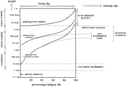
Figure 2.24: Effects on crack initiation and crack growth period ... 32

Figure 2.25: Surface effect on S-N curve, plotted on logarithmic scale ... 33

Figure 2.26: The three stages of fatigue failure ... 35

Figure 2.27: Grain boundary effect on crack growth in an Aluminum alloy ... 35

Figure 2.28: Top view of crack with crack front passing through many grains ... 36

Figure 2.29: Different stages of fatigue life and relevant factors ... 37

Figure 2.30: Different scenarios of fatigue crack growth ... 38

Figure 2.31: Inhomogeneous stress distribution due to elastic anisotropy ... 39

Figure 2.32: Hysteresis loops with and without mean stress and strain ... 41

Figure 2.33: Cyclic ratcheting-stress controlled ... 42

Figure 2.34: Hysteresis loops with different mean stresses ... 47

Figure 2.35: Total strain-life curve ... 48

Figure 2.36: Average ratio of fully reversed (R = -1) long-life fatigue strengths ... 53

Figure 2.38: The transition temperature revealed by impact tests on Charpy V-notched

specimens of low carbon steel ... 57

Figure 2.39: Two Charpy V-notched specimens, thickness 10 mm ... 58

Figure 3.1: Microstructure of G40.21 350WT steel (as received) ... 66

Figure 3.2: The geometry, assembly and mounting of test specimen ... 68

Figure 3.3: Surface preparation of specimens ... 69

Figure 3.4: Infrared thermometer used in detecting temperature difference regions ... 70

Figure 3.5: The tension test processes sequence ... 70

Figure 3.6: The system limits in room temperature tests ... 72

Figure 3.7: a) Uniform-gauge and b) hourglass test sections ... 74

Figure 3.8: The fatigue test processes sequence ... 77

Figure 3.9: The fatigue test as set in the MTS controller system... 78

Figure 3.10: Strain rate estimation ... 80

Figure 3.11: Low temperature fatigue test apparatus with environmental chamber ... 81

Figure 4.1: Stress-strain plots of AISI 1022 HR steel ... 86

Figure 4.2: Stress-strain plots of G40.21 350WT steel in room temperature ... 87

Figure 4.3: Quasi-static relationships of G40.21 steel in various temperatures ... 88

Figure 4.4: Effect of mean strain on tensile strength of AISI 1022 HR steel ... 89

Figure 4.5: Effect of mean strain on tensile strength for G40.21 350WT steel ... 90

Figure 4.7: Effect of temperature on tensile strength of G40.21 350WT steel... 92

Figure 4.8: Effect of mean strain on yield strength for AISI 1022 HR steel ... 93

Figure 4.9: Effect of mean strain on yield strength of G40.21 350WT steel ... 93

Figure 4.10: Effect of strain amplitude on yield strength of G40.21 350WT steel ... 94

Figure 4.11: Effect of temperature on yield strength of G40.21 350WT steel ... 95

Figure 4.12: Effect of mean strain on fracture strength for AISI 1022 HR steel ... 96

Figure 4.13: Effect of mean strain on fracture strength of G40.21 350WT steel ... 97

Figure 4.14: Effect of strain amplitude on fracture strength of G40.21 350WT steel .... 98

Figure 4.15: Effect of temperature on fracture strength of G40.21 350WT steel ... 99

Figure 4.16: Effect of mean strain on percentage elongation of AISI 1022 HR steel .. 100

Figure 4.17: Effect of mean strain on percentage elongation of G40.21 350WT steel . 101 Figure 4.18: Effect of strain amplitude on percentage elongation of G40.21 steel ... 102

Figure 4.19: Effect of temperature on percentage elongation of G40.21 350WT steel 103 Figure 4.20: Effect of mean strain on per. reduction in area of AISI 1022 HR steel .... 104

Figure 4.21: Effect of mean strain on percentage reduction in area of G40.21 steel ... 104

Figure 4.22: Effect of strain amplitude on per. reduction in area of G40.21 steel... 105

Figure 4.23: Effect of temperature on percentage reduction in area of G40.21 steel ... 106

Figure 4.24: Effect of mean strain on toughness for AISI 1022 HR steel ... 107

Figure 4.25: Effect of mean strain on toughness of G40.21 350WT steel ... 108

Figure 4.27: Effect of temperature on toughness of G40.21 350WT steel ... 110

Figure 4.28: Stress softening and mean stress relaxation of AISI 1022 HR and G40.21 350WT steels ... 111

Figure 4.29: Effect of temperature on stress softening and mean stress relaxation of G40.21 350WT steel... 112

Figure 4.30: Hysteresis loops of AISI 1022 HR steel in room temperature ... 113

Figure 4.31: Hysteresis loops of G40.21 350WT steel in room temperature ... 114

Figure 4.32: Effect of strain amplitude on hysteresis loops of G40.21 steel in RT ... 115

Figure 4.33: Hysteresis loops of G40.21 350WT steel in +25 ºC and -30 ºC ... 116

Figure 4.34: Mean strain-life diagram of AISI 1022 HR and G40.21 350WT steels ... 122

Figure 4.35: Strain-life diagram of G40.21 350WT steel... 123

Figure 4.36: Life-temperature relationship of G40.21 350WT steel... 124

Figure 4.37: Temperature difference detection using infrared thermometer ... 125

Figure 5.1: The regression models derived by Microsoft Excel software ... 137

Figure 5.2: Relationship between post-cyclic and monotonic tensile strength ... 142

Figure 5.3: Relationship between post-cyclic tensile strength and number of cycles ... 143

Figure 5.4: Relationship between post-cyclic tensile strength and mean strain ... 143

Figure 5.5: Relationship between post-cyclic tensile strength and strain amplitude .... 144

Figure 5.6: Relationship between post-cyclic tensile strength and temperature ... 144

Figure 5.7: Multiple linear regression model of the post-cyclic tensile strength ... 148

Figure 5.9: Data entry in Eureqa II software ... 152

Figure 5.10: Selection of arithmetic functions in Eureqa II software ... 153

Figure 5.11: Start search for solution in Eureqa II software... 154

Figure 5.12: View results in Eureqa II software software ... 154

Figure 5.13: Predicted and observed tensile strengths of G40.21 steel-G1 ... 156

Figure 5.14: Predicted and observed tensile strengths of G40.21 steel-G2 ... 157

Figure 5.15: Predicted and observed tensile strengths of G40.21 steel-G3 ... 157

Figure 5.16: Predicted and observed tensile strengths of both steels (A1 and G1) .... 159

Figure 5.17: Universal regression model of tensile strength for both steels ... 161

Figure 5.18: Universal reg. model of tensile strength for G40.21 steel-strain history .. 162

Figure 5.19: Universal regression model of tensile strength for G40.21 steel-temp ...163

Figure 5.20: Universal regression model of yield strength for both steels ... 165

Figure 5.21: Universal reg. model of yield strength for G40.21 steel-strain history .... 166

Figure 5.22: Universal reg. model of yield strength for G40.21 steel-temperature ... 166

Figure 5.23: Universal regression model of fracture strength for both steels ... 168

Figure 5.24: Universal reg. model of fracture strength for G40.21 steel-strain history 168

Figure 5.25: Universal reg. model of fracture strength for G40.21 steel-temperature .. 169

Figure 5.26: Universal regression model of toughness for both steels ... 170

Figure 5.27: Universal reg. model of toughness for G40.21 steel-strain history ... 171

Figure 5.29: Universal regression model of elongation for both steels... 172

Figure 5.30: Universal reg. model of elongation for G40.21 steel-strain history ... 173

Figure 5.31: Universal regression model of elongation for G40.21 steel-temperature . 173

Figure 5.32: Universal regression model of reduction in area for both steels ... 174

Figure 5.33: Universal reg. model of reduction in area for G40.21 steel-strain history 175

Figure 5.34: Universal reg. model of reduction in area for G40.21 steel-temperature . 175

Figure 5.35: The 95% confidence bands for the ε-N curve of G4.21 steel... 185 Figure 6.1: Specimen geometry according to ASTM standards E8 and A370 ... 188

Figure 6.2: Screen shot of mesh generated using C3D4 elements ... 190

Figure 6.3: ABAQUS results of specimen subjected to strain of 1000 µε ... 198 Figure 6.4: ABAQUS results of specimen subjected to strain of 1100 µε ... 198 Figure 6.5: Screen shot of fe-safe software interface ... 202 Figure 6.6: Fatigue peak-valley and Hysteresis loops ... 206

Figure 6.7: The four nodes tetrahedral element ... 207

Figure 6.8: The sinusoidal loading signal in fe-safe with zero mean strain, strain

amplitude of 2400 µε, and frequency of 5.0 Hz ... 208

LIST OF APPENDICES

Appendix A: AMERICAN BUREAU OF SHIPPING (ABS) ... 229

Appendix B: AMERICAN SOCIETY FOR TESTING AND MATERIALS (ASTM) 237

Appendix C: CANADIAN STANDARDS ASSOCIATION (CSA) ... 238

Appendix D: DET NORSKE VERITAS (DNV) AND (IACS) ... 244

Appendix E: EMPIRICAL FORMULAE ... 249

Appendix F: STATISTICAL ANALYSES OF STRAIN-LIFE RELATIONSHIP ... 260

Appendix G: NUMERICAL MODELING OF STRAIN-LIFE RELATIONSHIP ... 264

CHAPTER 1: INTRODUCTION

The mechanical behaviour of fatigue-damaged material is expected to differ from that of damage-free material. This change in mechanical behaviour during service of engineering structures and components may lead to unforeseen premature failure. The change in materials behaviour in terms of tensile properties of metals and alloys was reported by a few earlier studies. However, there is no data for many materials which are widely used in the engineering applications. Furthermore, the trend of change (increase or decrease) in tensile properties is dependent on the material type, data of previous materials might not be useful in assessing the behaviour of other materials. The objectives of this study were set after completion of a detailed literature review. Accordingly, equipments, materials required, and other requirements were decided. Two steels were chosen in this study and these are: G40.21 350WT which is used in ship hull structures and AISI 1022 HR which is used in general structural applications.

1.1SCOPE OF THE WORK

Any study should have reasonable causes to let researchers take decision to carry it out. The outcome should be in the stream of the public needs which is represented in this study by the industry of structural steels and the related applications. The following are the scope of work of this dissertation.

a) The importance of mechanical properties and their changes due to application of cyclic loads. These changes should be studied and recorded to aid the design process for reducing or avoiding the possibility of fatigue damages. This study intended to achieve this through experimental tests.

b) The scope of work also included derivation of empirical formulae for prediction of the changes in mechanical properties of fatigue-damaged structural steels. These formulae could be a tool to reduce the cost of experimentally investigating these changes.

d) The strain-life theories were used by researchers to predict fatigue life numerically. These theories are dependent on parameters called the strain-life fatigue parameters. Several methods are available for the calculation of these parameters. The current study intended to assess the methods for calculating strain-life fatigue parameters and recommend usage of the most accurate method(s).

e) There is a little information available on fatigue behaviour of materials at low temperatures. This study decided to take a bold step to understand how zero and sub-zero temperatures influence mechanical properties and fatigue life of steels.

1.2 OBJECTIVES OF THE STUDY

The current study was carried out to investigate the influence of strain-controlled cyclic loading on the mechanical behaviour and fatigue life of structural steels in room and low temperatures. A large number of material tests were undertaken to examine these effects and to achieve the following objectives.

1) Study the mechanical behaviour of two steels under strain-controlled cyclic loading in room and low temperatures.

2) Compare the mechanical behaviour of the two fatigue-damaged steels and determine the effect of various parameters of cyclic loading.

3) Determine the experimental strain-life relationships for both steels. 4) Study the effect of temperature on fatigue life experimentally.

5) Derive empirical formulae for predicting the mechanical behaviour of both steels. 6) Study the appropriate method(s) for calculation the strain-life fatigue parameters

that used in the numerical model of estimating fatigue life.

7) Analyse the strain-life relationships statistically to determine if the experimental data falls within desired confidence bands and also determine the validity of fatigue-life linear model.

1.3PREVIOUS STUDIES

studies are conducted by: López et al. (2011) on Titanium alloy, Sánchez-Santana et al. (2008) on 6061-T6 aluminum alloy and AISI 4140T steel, Grenier et al. (2007) on AISI 1018 steel, Ghosh (2001) on En 17 steel, and Rudenko and Splvakov (1975) on 16GNMA steel. More details are provided in section 2.2.5.

There are other studies conducted to show the low temperature effect on the monotonic and fatigue behaviour of materials. These studies are detailed in section 2.4.1.

1.4METHODOLOGY

The current study was completed using experimental, statistical, and numerical analyses. The objectives of this study were achieved through the following procedure.

a) Manufacturing test specimens using AISI 1022 HR and G40.21 350WT steels according to ASTM standards E8, A370 and E606.

b) Grouping the specimens in compliance with the experimental design principles. c) Performing quasi-static tensile tests in room and low temperatures to determine

the mechanical properties of the monotonic (damage-free) steels.

d) Applying strain-controlled axial cyclic loading tests to a pre-determined cycle count, followed by the application of quasi-static tensile tests to determine the mechanical properties of post-cyclic (fatigue-damaged) steels.

e) Analysing the experimental results to determine the changes in mechanical properties of the post-cyclic steels.

f) Deriving empirical formulae to predict the mechanical behaviour of both steels using relevant parameters.

g) Conducting fatigue life tests to plot the experimental strain-life relationship of both steels.

h) Conducting fatigue life tests of G40.21 350WT steel at low temperatures to determine the effect of low temperatures on the fatigue life.

i) Analysing the strain-life relationship statistically to determine the validity of the linear model, examining the experimental data with confidence levels, and estimating the scatter factor.

CHAPTER 2: LITERATURE REVIEW

In this chapter, a detailed review of the effect of cyclic loading on the materials behaviour was presented. First, crystallography including materials atomism, lattice structure, defects, deformations and response to external loads was discussed. This preview will assist in understanding the changes in materials properties. Then fatigue concept including crack initiation, propagation, and fracture mechanism was discussed. Subsequently, fatigue-life theories were presented focusing on strain-life theories. Finally, environmental effects including low and elevated temperatures effects on materials subjected to static and cyclic loads was discussed.

2.1 MATERIAL RESPONSE

For better understanding the effect of cyclic loading on mechanical properties of material, it is essential first to understand crystallographic changes due to applying load, statically and cyclically.

2.1.1 Crystallography

Crystallography is the experimental science of determining the arrangement of atoms in solids. It represents a tool that is often employed by materials scientists. When performing any process on a material, it may be desired to find out what compounds and what phases are present in the material. Crystallography is useful in phase identification. Each phase has a characteristic arrangement of atoms. Techniques such as X-ray diffraction can be used to identify which patterns are present in the material, and thus which compounds are present [Snigirev, 2007].

2.1.1.1 Atomism

An atom is the smallest unit quantity of an element that is capable of existence whether alone or in chemical combination with other atoms of the same or other elements.

electrical conductivity, some mechanical properties, the nature of interatomic bonding, atom size, and optical characteristics [DeGarmo et al., 2003].

The atoms vary in volume from element to another, for example in the periodic table the calculated radius of the Helium atom is 31 pm (picometres, where pm=10-12 m) and the one of Cesium atom is 298 pm, while Iron atom has a calculated radius of 156 pm.

Atoms Arrangements in Materials: Atoms usually bond to other atoms in some manner

as a result of interatomic forces. As atoms bond together to form aggregates, it was found that the particular arrangement of atoms has a significant effect on the material properties. Depending on the manner of atomic grouping, materials are classified as having molecular structures, crystal (crystalline) structures, or amorphous (glassy or non-crystalline) structures.

Solid metals (such as steel) and most minerals have a crystalline structure. Here the

atoms are arranged in a three-dimensional geometric array known as a lattice. Lattices are

describable through a unit building block, or unit cell, that is essentially repeated throughout space [Black and Kosher, 2008].

If materials are compared according to their atomic structures, body-centered cubic (bcc) metals offer high engineering strength. Face-centered cubic (fcc) structure is the preferred structure for many engineering metals and tends to provide exceptionally high ductility (the ability to be plastically deformed without fracture). The metals having the hexagonal close-packed (hcp) structure tend to have poor ductility, fail in a brittle manner, and often require special processing procedures [Black and Kosher, 2008].

For more information regarding atomism see the following references: [Leigh, 1990, DeGarmo et al., 2003, Kamrani et al., 2006, and Snigirev, 2007].

2.1.1.2 Crystallite

A crystallite is a domain of solid-state matter that has the same structure as a single crystal. Metallurgists often refer to crystallites as "grains". Most materials are

polycrystalline; they are made of a large number of single crystals-crystallites-held

The number and size of the grains in a metal vary with the rate of nucleation and the rate of growth. The greater the nucleation rate, the smaller the resulting grains. Because the resulting grain size will influence certain mechanical and physical properties (such as yield strength, refer to Hull-Petch relationship), that rate should be controlled properly. One means of specification is through the ASTMgrain size number, defined as: N= 2n-1

where N is the number of grains per square inch visible in a prepared specimen at l00X magnification, and n is the ASTM grain-size number. Low ASTM numbers (n) mean a few massive grains, while high numbers refer to materials with many small grains [Black and Kosher, 2008].

2.1.2 Crystallographic Defects

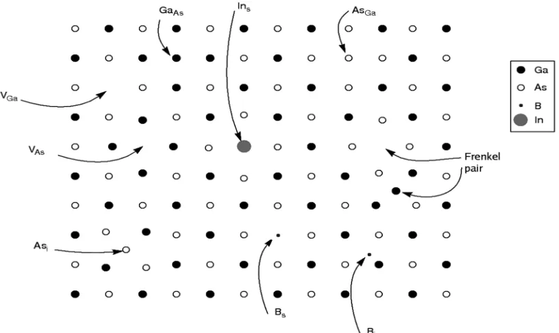
Most crystalline materials are not perfect: the regular pattern of atomic arrangement is interrupted by crystallographic defects. These defects may be point, line, planar or bulk defects as explained below. Crystallographic defects play a significant role in mechanical properties changes (i.e. dislocations, or barriers for dislocations movement) as well as sites for fatigue crack initiation and micro crack barriers.

2.1.2.1 Point Defects are defects which are not extended in space in any direction. There

is no strict limit for how small a "point" defect should be, but typically the term is used to describe defects which involve at most a few extra or missing atoms without an ordered structure of the defective positions. Larger defects in an ordered structure are usually considered dislocation loops. For historical reasons, many point defects especially in ionic crystals are called “centers”: for example the vacancy in many ionic solids is called an F-center. Types of point defects are mentioned bellow:

• Vacancies are sites which are usually occupied by an atom but which are

can form better bonds with atoms in the other directions. A vacancy (or pair of vacancies in an ionic solid) is sometimes called a Schottkydefect.

• Interstitialsare atoms which occupy a site in the crystal structure at which there is

usually not an atom. They are generally high energy configurations. Small atoms in some crystals can occupy interstices without high energy, such as hydrogen in palladium.

• A nearby pair of a vacancy and an interstitial is often called a Frenkel defect or

Frenkel pair. This is caused when an ion moves into an interstitial site and

creates a vacancy.

Figure (2.1) Schematic illustration of some simple point defect types in a monatomic

solid [Knordlun at en.wikipedia] permission released into the public domain by the

author in 3-3-2007

• Impurities occur because materials are never 100% pure. In case of an impurity,

the atom is often incorporated at a regular atomic site in the crystal structure. This is neither a vacant site nor is the atom on an interstitial site and it is called a

substitutional defect. The atom is not supposed to be anywhere in the crystal, and

is thus an impurity.

• Antisite defects occur in an ordered alloy or compound. For example, some alloys

illustration assume that type A atoms sit on the corners of a cubic lattice, and type B atoms sit in the center of the cubes. If one cube has an A atom at its center, the atom is on a site usually occupied by an atom, but it is not the correct type. This is neither a vacancy nor an interstitial, nor an impurity [Mattila and Nieminen, 1995 and Hausmann et al., 1996].

Figure (2.2) Schematic illustration of defects in a compound solid, using GaAs as an

example [Knordlun at en.wikipedia] permission released into the public domain by the

author in 3-3-2007

2.1.2.2 Line Defects: Dislocations are linear defects around which some of the atoms of

the crystal lattice are misaligned [Hirth and Lothe, 1992]. The presence of dislocations strongly influences many of the properties of materials. The theory was originally developed by Vito Volterra in 1905 [Reed-Hill, 1994]. There are two basic types of dislocations, edge dislocation and screw dislocation. However, third type called mixed dislocation may form as a combination of the first two types.

a) Edge dislocations are caused by the termination of a plane of atoms in the middle of a

perfectly ordered on either side. The analogy with a stack of paper is apt: if a half a piece of paper is inserted in a stack of paper, the defect in the stack is only noticeable at the edge of the half sheet.

Figure (2.3) The edge dislocation. The dislocation line is presented in blue, the

Burgers vector b in black [Wikityke at en.wikipedia] permission: CC-BY-SA-2.5;

Released under the GNU Free Documentation License

b) Screw dislocation is a partial tearing of the crystal plane [Black and Kosher, 2008]. It

is more difficult to visualise, but basically comprises a structure in which a helical path is traced around the linear defect (dislocation line) by the atomic planes of atoms in the crystal lattice (see Figure 2.4).

Figure (2.4) Schematic diagram (lattice planes) showing a screw dislocation [Javier

B. Vílchez] permission released into the public domain by the author in 27-1-2007

parallel. In metallic materials, b is aligned with close-packed crystallographic directions and its magnitude is equivalent to one inter-atomic spacing.

c) In many materials, dislocations are found where the line direction and Burger’s vector

are neither perpendicular nor parallel and these dislocations are called mixed dislocations, consisting of both screw and edge character, as shown in Figure (2.5). The mixed dislocation is the most popular type in the metallic materials. The theory and

mechanism of dislocation are explained in section 2.1.3.3. Dislocations can be observed experimentally using transmission electron microscopy (TEM), field ion microscopy and atom probe techniques.

Figure (2.5) The mixed dislocation [www.courses.eas.ualberta.ca]

Looking at the appearance of variation in the observed grains, in Figure (2.6a) the dislocation structures of grains vary greatly among grains, while in Figure (2.6c) all grains have relatively uniform dislocation cell structures. These observations suggest that cyclic loading with larger strain amplitudes lead to a qualitatively more uniform dislocation cell structure, and similar results have been reported elsewhere [Mayama et al., 2008].

Mayama et al. study prove that cyclic loading leads to dislocation movement from grain interior to the boundaries (which plays a barrier to the dislocation transferring to adjacent grain); subsequently higher driving force will be required to perform a particular strain.

2.1.2.3 Planar Defects

• Grain boundaries occur where the crystallographic direction of the lattice

abruptly changes. This usually occurs when two crystals begin growing separately and then meet.

• Anti-phase boundaries occur in ordered alloys: in this case, the crystallographic

direction remains the same, but each side of the boundary has an opposite phase: For example if the ordering is usually ABABABAB, an anti phase boundary takes the form of ABABBABA.

• Stacking faults occur in a number of crystal structures, but the common example

is in close-packed structures. Face-centered cubic (fcc) structures differ from hexagonal close packed (hcp) structures only in stacking order: both structures have close packed atomic planes with six fold symmetry, the atoms form equilateral triangles. When stacking one of these layers on top of another, the atoms are not directly on top of one another, the first two layers are identical for hcp and fcc, and labelled AB. If the third layer is placed so that its atoms are directly above those of the first layer, the stacking will be ABA-this is the hcp structure, and it continues ABABABAB (see Figure 2.7). However there is another location for the third layer, such that its atoms are not above the first layer. Instead, the fourth layer is placed so that its atoms are directly above the first layer. This produces the stacking ABCABCABC, and is actually a cubic arrangement of the atoms. A stacking fault is a one or two layer interruption in the stacking sequence, for example if the sequence ABCABABCAB were found in an fcc structure [Hirth and Lothe, 1992].

Figure (2.7) hcp lattice (left) and fcc lattice (right) [Twisp] permission released

2.1.2.4 Bulk Defects

• Voids are small regions where there are no atoms, and can be thought of as

clusters of vacancies.

• Impurities can cluster together to form small regions of a different phase. These

are often called precipitates.

Porosity: Pores are holes or cavities in the metal. A major cause is the decrease in

volume, typically of the order of 10 % when liquid transforms to solid. Holes are formed when pockets of liquid are isolated inside the solid, for example, in the interdendritic spaces. The size of pores, or shrinkage cavities, is proportional to that of the original liquid pocket. Small pores, less than about a micron in size, are generally harmless. Larger ones may subsequently be closed during hot working of the cast product.

2.1.3 Deformation:

2.1.3.1 Elastic Deformation:

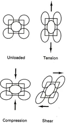
An understanding of mechanical behaviour begins with understanding the way crystals react to mechanical loads. Most studies start with carefully prepared single crystals. Through these studies we learn that the mechanical behaviour is dependent on: (1) the type of lattice, (2) the interatomic forces (i.e., bond strength), (3) the spacing between adjacent planes of atoms, and (4) the density of atoms on the various planes.

If the applied loads are relatively low, the crystals respond by simply stretching or compressing the distance between atoms as shown in Figure (2.8). The basic lattice unit does not change, and all of the atoms remain in their original positions relative to one another. The applied load serves only to alter the force balance of the atomic bonds, and the atoms assume new equilibrium positions with the applied load as an additional component of force. If the load is removed, the atoms return to their original positions and the crystal resumes its original size and shape. The mechanical response is elastic in

nature, and the amount of stretch or compression is directly proportional to the applied load or stress.

strain is known as Poisson's ratio. This value is always less than 0.5 and is usually about 0.3 for steels [Black and Kosher, 2008].

Figure (2.8) Distortion of a crystal lattice in response to various elastic loadings

[Black and Kosher, 2008]

2.1.3.2 Plastic Deformation

As the magnitude of applied load becomes greater, distortion (or elastic strain) continues to increase, and a point is reached where the atoms either (1) break bonds to produce a fracture, or (2) slide over one another in a way that would reduce the load. For metallic materials, the second phenomenon generally requires lower loads and occurs preferentially. The atomic planes shear over one another to produce a net displacement or permanent shift of atom positions, known as plastic deformation. Conceptually, this is similar to the distortion of a deck of playing cards when one card slides over another. The actual mechanism, however, is really a progressive one rather than one in which all of the atoms in a plane shift simultaneously. More significantly, however, the result is a permanent change in shape that occurs without a concurrent deterioration in properties.

having the highest atomic density and greatest separation. The rationale for this can be seen in the simplified two-dimensional array of Figure 2.9. Planes A and A' have higher density and greater separation than planes B and B'. In visualizing relative motion, we see that the atoms of B and B' would interfere significantly with one another, whereas planes A and A' do not experience this difficulty.

Figure (2.9) Simple schematic illustrating the lower deformation resistance of planes with higher atomic densities and larger inter-planar spacing [Black and Kosher,

2008]

Although Figure 2.9 represents the planes of sliding as lines, crystal structures are actually three-dimensional. Within the preferred planes are also preferred directions. If sliding occurs in a direction that corresponds to one of the close-packed directions (shown as dark lines in Figure 2.10), atoms can simply follow one another rather than each having to negotiate its own path. Plastic deformation therefore, tends to occur by the preferential sliding of maximum-density planes (close-packed planes if present) in directions of closest packing. The specific combination of plane and direction is called a

slip system, and the resulting shear deformation or sliding is known as slip.

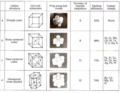
The ability to deform a given metal depends on the ease of shearing one atomic plane over an adjacent one and the orientation of the plane with respect to the applied load. Consider, for example, the deck of playing cards. The deck will not "deform" when laid flat on the table and pressed from the top or when stacked on edge and pressed uniformly. The cards will slide over one another, however, if the deck is skewed with respect to the applied load so as to induce a shear stress along the plane of sliding. With this understanding, consider the deformation properties of the three most common crystal structures: BCC, FCC, and HCP.

a) Body-centered cubic: In the bcc structure, there are no close-packed planes. Slip

Figure (2.11) Comparison of the crystal structures: simple cubic, body-centre cubic,

face-centre cubic and hexagonal close-packed [Black and Kosher, 2008]

Figure (2.12) Slip planes of the various lattice types [Black and Kosher, 2008] c) Hexagonal close-packed: The hexagonal lattice also contains close-packed planes, but only one such plane exists within the lattice. Although this plane contains three close-packed directions and the force required to produce slips again rather low, the probability of favorable orientation to the applied load is small (especially if one considers a polycrystalline aggregate). As a result, metals with the hcp structure tend to have low ductility and are often classified as brittle [Black and Kosher, 2008].

Figure (2.13) Schematic representation of slip and crystal rotation resulting from deformation [Black and Kosher, 2008]

2.1.3.3 Dislocation Theory of Slippage

certain engineering metal. Barriers to dislocation motion tend to increase the overall strength of a metal. These barriers take the form of other crystal imperfections and may be of point type, line, or surface type (see sec 2.1.2 crystallographic defects) [Black and Kosher, 2008].

One should note that the slip lines do not cross from one grain to another. The grain boundaries act as barriers to the dislocation motion. Therefore, metals with a finer grain structure more grains per unit area tend to exhibit greater strength and hardness, coupled with increased impact resistance. This near-universal enhancement of properties is an attractive motivation for grain size control during processing [Black and Kosher, 2008].

Dislocations can move if the atoms from one of the surrounding planes break their bonds and re-bond with the atoms at the terminating edge as shown in Figure (2.14) below. It is the presence of dislocations and their ability to readily move (and interact) under the influence of stresses induced by external loads that leads to the characteristic malleability of metallic materials.

Figure (2.14) The movement of edge dislocation through the crystal [www.

ic.arizona.edu]

Extra plane of atoms in crystal

This row of bonds will break and reattach itself to a different row of atoms. It is much easier for only one row of bonds to break and reform than for an entire plane of bonds (i.e. the bonds intersecting the pink line) to do so.

Edge dislocation Edge dislocation

2.1.3.4 Stress-strain Curve: Ductile Materials

Steel generally exhibits a very linear stress–strain relationship up to a well defined yield point (Figure 2.15). The linear portion of the curve is the elastic region and the slope is the modulus of elasticity or Young's Modulus. After yield point, the curve typically decreases slightly because of dislocations escaping from Cottrell atmospheres (see the explanation of Cottrell atmospheres on the next page). As deformation continues, the stress increases on account of strain hardening until it reaches the ultimate strength. Until this point, the cross-sectional area decreases uniformly because of Poisson contractions. The actual rupture point is in the same vertical line as the visual rupture point.

However, beyond this point a neck forms where the local cross-sectional area decreases more quickly than the rest of the sample resulting in an increase in the true stress. On an engineering stress-strain curve this is seen as a decrease in the stress (curve A in Figure 2.15). Conversely, if the curve is plotted in terms of true stress and true strain the stress will continue to rise until failure (curve B in Figure 2.15). Eventually the neck becomes unstable and the specimen ruptures (fractures).In Figure (2.15) the numbers: 1. Ultimate strength, 2. Yield strength, 3. Rupture, 4. Strain hardening region, 5. Necking region, A: Engineering (apparent) stress, (F/A0), B: True (actual) stress (F/A)

Figure (2.15)A stress–strain curve typical of structural steel [David Richfield, 2009]

Permission is granted to copy, distribute and/or modify this document under the terms of the GNU* Free Documentation License

Cottrell atmospheres:

The concept of the Cottrell atmosphere was introduced by Cottrell and Bilby in 1949 to explain how dislocations are pinned in some metals by carbon or nitrogen interstitials. Cottrell atmospheres occur in body-centered cubic (bcc) materials, such as iron or nickel, with small impurity atoms, such as carbon or nitrogen. As these interstitial atoms distort the lattice slightly, there will be an associated residual stress field surrounding the interstitial. This stress field can be relaxed by the interstitial atom diffusing towards a dislocation, which contains a small gap at its core (as it is a more open structure), see Figure 2.16. Once the atom has diffused into the dislocation core the atom will stay. Typically only one interstitial atom is required per lattice plane of the dislocation.

Figure 2.16 A carbon atom below a dislocation in iron, forming a Cottrell

atmosphere [Cottrell and Bilby, 1949]

Once a dislocation has become pinned, a small extra force is required to unpin the dislocation prior the yielding, producing an observed upper yield point in a stress-strain curve. After unpinning, dislocations are free to move in the crystal, which results in a subsequent lower yield point, and the material will deform in a more plastic manner. Leaving the sample to age, by holding it at room temperature for a few hours, enables the carbon atoms to re-diffuse back to dislocation cores, resulting in a return of the upper yield point.

Cottrell atmospheres lead to formation of Luder’s Bands and large forces for deep drawing and forming large sheets, making them a hindrance to manufacture. Some steels are designed to remove the Cottrell atmosphere effect by removing all the interstitial atoms. Steels such as Interstitial Free Steel are decarburized and small quantities of titanium are added to remove nitrogen [Cottrell and Bilby, 1949].

2.1.3.5 Stress-strain Curve: Brittle Materials

strength is negligible compared to the compressive strength and it is assumed zero for many engineering applications.

Figure (2.17) Stress-strain curve for brittle materials. Permission is granted to copy,

distribute and/or modify this document under the terms of the GNU Free Documentation License

2.1.3.6 Cyclic Stress-strain Curves

The changes in mechanical properties of a material due to cycle-dependent responses are observed by producing a cyclic stress-strain curve. Cyclic stress-strain curves often refers to the stress-strain relationship obtained by the material once cycle-dependent stabilization has occurred, that is, once plastic shakedown has occurred [Bannantine et al., 1990]. There are various methods of determining the cyclic stress-strain curve, and there are small differences in the results from different methods. In reality, there exist multiple cyclic stress-strain curves at various levels of fatigue damage [Sandor, 1972]. However, the quasi-static tensile tests method was found to be the most efficient at determining the cyclic stress-strain curves at various levels of fatigue damage. From here on, cyclic stress-strain curves refer to the stress-strain relationship obtained at any arbitrary amount of fatigue damage within the material’s fatigue life, and not only once a cycle-dependent stabilization has occurred.

curve of a material with the same composition, size, shape, and initial conditions as that of the virgin specimen. Line B is above line A indicating that the material hardened from one cycle to the next and is more resistant to deformation. Therefore, a higher stress level than that of the virgin specimen is required to generate a given strain. On the other hand, line C represents a cyclic stress-strain curve of a material that softened from one cycle to the next and is more susceptible to deformation. Therefore, a lower stress level is required to generate a given strain.

Figure (2.18) Cycle-dependent changes in stress-strain response [Sandor, 1972]

The cyclic stress-strain expression of Ramberg–Osgood is usually used to fit the

strain-life curve. The stress amplitudes, σa, and plastic strain amplitudes, εpa, from the stable

stress-strain hysteresis loops (plastic shakedown) are being employed along with the corresponding cyclic fatigue life Nf for each test [Dowling 2009].

For cyclic stress-strain curve

For hysteresis loop

+ 2

∆/́ _(2.2) Where :

́:

́/ and ́ =

B

A

C

Stress

́ : fatigue strength coefficient (MPa);

́ : fatigue ductility coefficient, which is the plastic strain amplitude at 2nf =1; b: fatigue strength exponent (Basquin’s exponent);

c: fatigue ductility exponent (Coffin-Manson exponent);

2.1.4 Cycle-dependent Material Response

The term ‘cycle-dependent’ refers to the behaviour observed by the material from one cycle to the next. When subjected to cyclic loads, materials respond in different ways depending on the specific loading conditions. Cycle-dependent hardening and cycle-dependent softening are two extreme changing responses demonstrating that these responses are not always constant from one cycle to the next. The materials’ responses (such as stress range or strain range) due to both cycle-dependent hardening and softening depend on whether the conditions are stress-controlled or are strain-controlled.

2.1.4.1 Cyclic Stress-strain Response

Figure (2.19) The sequence of processes during fatigue of metallic materials

[Mughrabi, 1985]

2.1.4.2 Stress-controlled Test

In a stress-controlled test, the stress limits remain constant from one cycle to the next while the strain is dependent on the applied stress. Cycle-dependent hardening occurs when the material is gradually increasing its resistance to deformation. Therefore, a decrease in the strain range occurs from cycle to cycle, indicating that the material has been work-hardened. Cycle-dependent softening occurs when the materials resistance to deformation gradually decreases from one cycle to the next. Therefore, the strain range increases from cycle to cycle during the application of a constant stress range. Figure 2.20 shows the cycle-dependent material responses occurring under a stress-controlled environment. As one of the three common fatigue-life methods (stress-life method, the strain-life method, and the linear-elastic fracture mechanics method), the stress-life method, based on stress levels only, is the least accurate approach, especially for low-cycle applications [Shigley, 2006].

2.1.4.3 Strain-controlled Test

In a strain-controlled test, the strain limits remain constant from cycle to cycle and the stress depends on the applied strain. As mentioned in the stress-controlled environment, a cycle-dependent hardening response refers to a gradually increasing resistance to deformation. Thus, in a strain-controlled environment, cycle-dependent hardening refers to a gradual increase in stress range required to accommodate for the constant strain range applied from cycle to cycle. Also, a gradual decrease in the stress range is a material response due to cycle-dependent softening. Figure (2.21) illustrates examples of cycle-dependent material response under a strain-controlled environment. The strain-life method involves more detailed analysis of the plastic deformation at

Figure (2.20)Stress-controlledcycle-dependent response [Sandor, 1972]

(a) Stress control function

(b) Cycle-dependent hardening

localized regions where the stresses and strains are considered for life estimates. This method is especially good for low-cycle fatigue applications [Shigley, 2006].

Figure (2.21) Strain controlled cycle-dependent response: (a) stress hardening, (b)

stress softening, (c) mean stress relaxation [ASM HDBK v19, 1996].

2.2 FATIGUE CONCEPT

Fatigue failure from the crystallographic point of view may consist of three stages: crack initiation, crack propagation or growth, and failure or rapture. Below are detailed explanations of these stages.

2.2.1 Crack Initiation

Because of operating cyclic stresses, a microcrack will nucleate within a grain of material. Crack initiation occurs from the material’s surface in most cases, so surface roughness plays a significant role in the crack initiation process. It is believed that the crystallography of a material has some influence on the mechanical behaviour during the crack initiation period. The crystallographic properties vary from one material to another, so the initial microcracking depends on the material type.

Fatigue crack initiation and crack growth are attributed to cyclic slip in slip bands. It implies cyclic plastic deformation as a result of moving dislocations. Fatigue occurs at stress amplitudes below the yield stress. At such a low stress level, plastic deformation is limited to a small number of grains of the material. This micro-plasticity can occur more easily in grains at the material surface because the surrounding material is present on one side only. The other side is the environment, usually a gaseous environment (e.g. air) or a liquid (e.g. sea water). As a consequence, plastic deformation in surface grains is less constrained than in subsurface grains; so it can occur at a lower stress level.

simply be removed from the slip step. Secondly, strain hardening in the slip band is also not fully reversible. As a consequence, reversed slip, although occurring in the same slip band, will occur on adjacent parallel slip planes. This is schematically indicated in Figure (2.22b). The same sequence of events can occur in the second cycle, see Figure (2.22) c and d.

Figure (2.22) Cyclic slip leads to crack nucleation [Schijve, 2004]

Figure (2.22) offers a simplified picture, but there are some points to be observed:

(i) A single cycle is sufficient to create a microscopic intrusion into the material, which in fact is a microcrack.

(ii) The mechanism occurring in the first cycle can be repeated in the second cycle, and in subsequent cycles and cause crack extension in each cycle.

(iii) The first initiation of a microcrack may well be expected to occur along a slip band. This has been confirmed by several microscopic investigations, see Figure (2.23). A slip band seen in Figure (2.23a) is actually a microcrack as confirmed in Figure (2.23b) after the band is opened by applying a 5% plastic strain to the material. A part of this slip band was already visible after no more than 0.5% of the fatigue life.