Performance Analysis of Load Balancing
Algorithms in Cloud Computing Environment
Dheeraj Pal Singh Brar1, Amanpreet Chawla1, Amar Singh1, Isha Chawla1
Assistant Professor, Department of CSE, SBS State Technical Campus, Ferozepur, Punjab, India1
ABSTRACT: Internet is the backbone of cloud computing. Cloud computing capabilities are available all over the network and accessible through internet in a ubiquitous manner. Although, a lot of research have been done in field of cloud computing, but it’s still in infancy and is faced with many issues and challenges. Some of have been discussed in this paper in brief such as load balancing, security, trust management, operating cost etc. This paper addresses the issue of load balancing and gives a brief description about various load balancing algorithms. This paper gives a proposal to make the existing algorithms more efficient and robust.
KEYWORDS: Cloud computing, Load balancing, Execution time.
I. INTRODUCTION
Mobile Ad Hoc Networks (MANETs) consists of a collection of mobile nodes which are not bounded in any infrastructure. Nodes in MANET can communicate with each other and can move anywhere without restriction. This non-restricted mobility and easy deployment characteristics of MANETs make them very popular and highly suitable for emergencies, natural disaster and military operations.
Cloud Computing is an emerging research field. There are many definitions of Cloud Computing proposed by different authors. According to the NIST definition of Cloud Computing, “Cloud computing is a model for enabling ubiquitous, convenient, on-demand network access to a shared pool of configurable computing resources (e.g., networks, servers, storage, applications, and services) that can be rapidly provisioned and released with minimal management effort or service provider interaction. This cloud model is composed of five essential characteristics, three service models, and four deployment models.”
Characteristics of cloud computing which adds to its popularity are: Broad network access, on-demand self-service, rapid elasticity, measured service, resource pooling. The service models of cloud computing are: IaaS (Infrastructure as a Service), which provide infrastructure to run and deploy the applications; PaaS (Platform as a Service), which provides programming tools and environments to install and run the applications; SaaS (Software as a Service), which provide access to the users to use the software installed on the cloud infrastructure. The deployment models of cloud computing are: private cloud, which is implemented solely for an organization and is managed and controlled by the organization or third party; community cloud, which is implemented by the group of one or more organizations that share common concerns (mission, shared concerns), public cloud, which is implemented for the general public and is managed and controlled by the organization offering cloud services; hybrid cloud, which is any combination of public, private and community cloud.
A. Challenges in Cloud Computing
There are various challenges in cloud computing such as:
2) Load Balancing: Cloud computing is an internet computing in which the load balancing is the one of the challenging tasks. Various optimization techniques are needed to make a balanced system by allocating the workload to the nodes in a manner that no node is overloaded or under loaded.
3) Energy Consumption: Cloud datacentres consume a lot of energy and release greenhouse gases. Google datacentre consumes energy equivalent to a city such as Sans Francisco. So, this is a serious issue, which demands not only the need to reduce the energy consumption but also to reduce the environment degradation.
4) Operating Cost: Cloud computing can have high costs due to it requirements for both an “always on” connection, as well as using large amounts of data back in-house.
II. LOADBALANCING
As the name suggests, “Load balancing means to balance the load of the entire system so that every node does equal amount of work”. Maximizing the resource utilization and minimizing the completion are the objectives, load balancing algorithm aims to achieve. Next, we will discuss about the categories of load balancing algorithms, the various performance parameters used to check the performance of a load balancing algorithm and the policies used in load balancing algorithm.
A. Categories of Load Balancing Algorithms
1. Depending on who initiated the process, load balancing algorithms can be of three categories: a) Server-initiated: If the load balancing algorithm is initialized by the sender.
b) Receiver-initiated: If the load balancing algorithm is initialized by the receiver.
c) Symmetric: It is the combination of both senders initiated and receiver initiated.
2. Depending on the current state of the system, load balancing algorithms can be of three categories:
a) Static Algorithms:Static algorithms divide the traffic equivalently between servers. By this approach the traffic on the servers will be disdained easily and consequently it will make the situation more imperfectly. This algorithm, which divides the traffic equally, is announced as a round robin algorithm. However, there were lots of problems appeared in this algorithm. Therefore, weighted round robin was defined to improve the critical challenges associated with round robin. In this algorithm, each server has been assigned a weight and according to the highest weight they received more connections. In the situation that all the weights are equal, servers will receive balanced traffic.
b) Dynamic Algorithms: Dynamic algorithms designated proper weights on servers and by searching in whole network a lightest server preferred to balance the traffic. However, selecting an appropriate server needed real time Communication with the networks, which will lead to extra traffic added to the system. In a comparison between these two algorithms, although round robin algorithms based on simple rule, more loads conceived for servers and thus imbalanced traffic discovered as a result. However; dynamic algorithm predicated on a query that can be made frequently on servers, but sometimes prevailed traffic will prevent these queries to be answered, and correspondingly more added overhead can be distinguished on the network.
B. Performance Parameters of Load Balancing Algorithms
Some of the parameters used to check the performance of a load balancing algorithm are:
1) Response Time: It can be measured as, the time interval between sending a request and receiving its response.
2) Throughput:The total numbers of tasks that have completed their execution is called throughput. High throughput is necessary for better performance.
3) Overhead:The overhead concerned with any load balancing algorithm indicates the extra cost involved in developing the algorithm.
4) Resource Utilization: It is the degree in which resources are utilized. This factor must be optimized to have an efficient load balancing algorithm.
5) Scalability:It determines the ability of an algorithm to perform uniform load balancing in a system with the increase in the number of nodes, according to the requirements.
C. Policies Used in Load Balancing Algorithms
There are various policies used in dynamic load balancing algorithms such as:
1) Transfer Policy: It selects the job to be transferred from the local node to some node at the remote place.
2) Selection Policy: It specifies the processes participating in load exchange.
3) Location Policy: The selection of the destination node for the transferred task is the location strategy.
4) Information Policy: It is responsible for collecting information about the nodes.
5) Load Estimation Policy: It tells how to estimate the load of any particular node.
6) Process Transfer Policy: It decides whether to execute the process locally or remotely.
7) Migration Limiting Policy: It defines the upper limit for process migration i.e. how many times a particular process can undergo migration.
III. COMPARISONOFDIFFERENTLOADBALANCINGALGORITHMS
A. Round Robin Algorithm
It is one of the simplest scheduling techniques that utilize the principle of time quantum. The time is divided into multiple interval and each node is given a particular time interval or time interval. Each node is given a quantum and in this quantum the node will perform its operations. The following algorithm shows the working of round robin. The algorithm depicts that each user request is served by every processor within given time quantum. When time interval is over, the next queued request will come for execution.
Algorithm:
1) Load Balancer maintains an index of VM's and state of the VM's (busy/available). At start all VM’s have zero allocation.
2) The datacentre controller receives the user requests. The requests are allocated to VM's on the basis of their states known from the VM queue. The load balancer will assign the time interval for user request execution.
3) The load balancer will calculate the turn- around time of process and also calculate the response time and average waiting time of user requests. It decides the scheduling order.
4) After the execution of cloudlets, the VMs are de- allocated by the Load Balancer.
5) The datacentre controller checks for new /pending/waiting requests in queue.
6) Continue from step-2.
B. Throtted Algorithm
In this algorithm, the load balancer maintains an index table of virtual machines and their states (Available or Busy). The client sends a request to data centre to find a suitable virtual machine (VM) to perform the recommended job. The data centre queries the load balancer for allocation of the VM. The load balancer scans the index table from top until the index table is scanned fully or the first available VM is found. If the VM is found, the VM id is send to the data centre. The data centre connects the request to the VM identified by the id. The data centre acknowledges the load balancer of the new allocation and the data centre revises the index table accordingly. While processing the client request, if suitable VM is not found, the load balancer returns -1 to the data centre. The data centre queues the request with it. When the VM completes the task, a request is acknowledged to data centre, which is further apprised to load balancer to de-allocate the same VM whose id is already communicated/connected.
Algorithm:
1) Throttled VM load balancer maintains an index table of VM and the state of the VM (BUSY/AVAILABLE). At the start all VM’s are idle.
2) Datacentre controller receives a new request.
3) Datacentre controller queries the Throttled VM load balancer for the next allocation.
4) Throttled VM load balancer parses the allocation table from top until the first available VM is found or the table is parsed completely. If found:
a) The throttled VM load balancer returns the VM id to the Datacentre controller.
c) Datacentre controller notifies the throttled VM load balancer of the new allocation.
d) Throttled VM load balancer updates the allocation table accordingly. If not found:
e) Throttled VM load balancer returns -1 and Datacentre controller stores the request in queue.
5) When the VM completes the task, the datacentre controller receives the response cloudlet, it notifies the throttled VM load balancer of the VM de-allocation.
6) The datacentre controller checks if there are any waiting requests in the queue then it continues from step 3.
C. Equally Spread Current Execution Algorithm
In this technique load balancer makes effort to preserve equal load to all the virtual machines connected with the data centre. This load balancer maintains an index table of Virtual machines and number of requests currently assigned to the Virtual Machine (VM). If the user request comes from the data centre to assign the new VM, it scans the index table for under-loaded VM. In case, more than one VM is found then first identified VM is chosen for handling the request of the client, the load balancer returns the VM id to the data centre controller. The data centre communicates the request to the VM identified by that id. The data centre increases the allocation count of identified VM and revises the index table. When VM completes the assigned job, a request is communicated to data centre which is further notified by the load balancer. The load balancer decreases the allocation count for identified VM by one and revises the index table but there is an additional computation overhead to scan the queue again and again.
Algorithm:
1) Find the available VM.
2) Check for all current allocation count is less than max length of VM list allocate the VM.
3) If available VM is not allocated create a new one.
4) Count the active load on each VM Return the id of those VM which is having least load.
5) The VM load balancer will allocate the request to one of the VM.
6) If a VM is overloaded, then the VM load balancer will distribute some of its work to the VM having least work so that every VM is equally loaded.
7) The datacentre controller receives the response to the request sent and then allocate the waiting requests from the job pool/queue to the available VM & so on.
8) Continue from step-2.
IV. SIMULATIONANDRESULTANALYSIS
The Simulation tool used is Cloud analyst.
A. Cloud Analyst
Cloud Analyst is tool that is used for modelling and simulation of cloud computing infrastructure and services (i.e. datacentre, virtual machines). The main features of Cloud Analyst are the following:
1) Easy to use Graphical User Interface (GUI): Cloud Analyst is equipped with an easy to use graphical user interface that enables users to set up experiments quickly and easily.
2) Graphical output: The Cloud Analyst is a GUI based tool which is developed on CloudSim architecture. 3) Use of consolidated technology and ease of extension: Cloud Analyst is based on a modular design that can be
easily extended. It is developed using these technologies: Java, CloudSim.
B. Main Components of Cloud Analyst
1) GUI Package: It is responsible for the graphical user interface, and acts as the front end controller for the application, managing screen transitions and other UI activities.
2) Simulation: This component is responsible for holding the simulation parameters, creating and executing the simulation.
3) User Base: This component models a group of users and generates traffic representing the users. 4) Datacentre Controller: This component controls the data centre activities.
6) VM Load Balancer: This component models the load balance policy used by data centres when serving allocation requests.
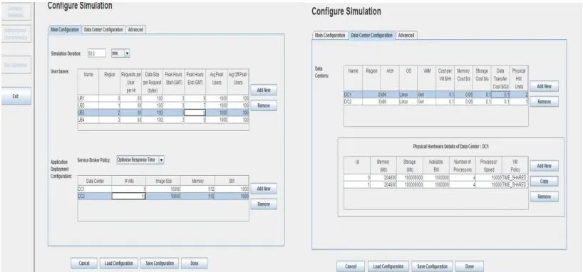
We have set the parameters for the application deployment configuration, data center configuration and user configuration as shown in figure1 and figure2and figure3respectively. The location of the user base defined in three regions as shown in figure2.
Figure 1: Simulation Screen in simulator Figure 2: Datacenter Configuration
We have taken the chosen two datacenter (DC1, DC2) to handle the user requests. One datacenter is located in region 0 and other is located at region 3. There are 5 VM's on DC1 and 6 VM's on DC2.Figure 2 shows the datacenter configuration and figure 3 shows the advance configurations and figure 4 shows the output screen of Cloud Analyst.
Figure 3: Advance Configuration Figure 4: Output Screen of Cloud Analyst
C. Comparative Results
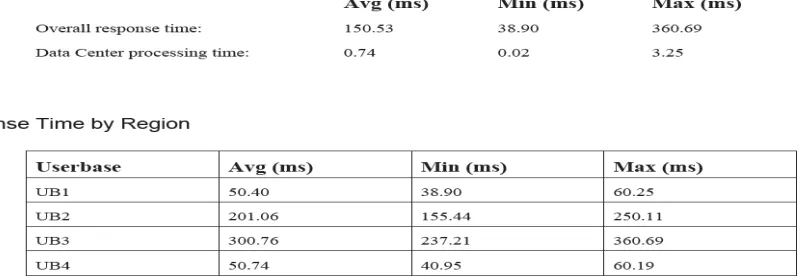
the overall response summery in the terms of the three main parameters that are minimum, maximum and the average response time in milliseconds.
Figure 5: Response time for the RR algorithm with 4 UB's
The figure 6, represents about the response time of the ESEC algorithm with the consideration of the four user bases that are UB1, UB2, UB3 and UB4. This also focuses values on the basis of four parameters like average response time, minimum response time and the maximum response time of the individual user base in milliseconds. Whereas figure 7 shows the values based on the TT algorithm based on the 4 user bases.
Figure 6: Response time for the ESEC algorithm with 4 UB's
Figure 7: Response time for the TT algorithm with 4 UB's
V. RESEARCHPROPOSALFORFUTUREWORK
In this paper, we surveyed the round robin (RR), ESEC and throttled algorithms for the load balancing in cloud computing. We discussed the challenges of cloud computing as well as discussed in brief about load balancing. In the future, we can develop the hybrid algorithm that contains the excellence of round robin and ESCE and Throttled algorithm. In the case of round robin (RR) algorithm, allocation takes place for a fixed time quantum but there are no set criteria to calculate the value of time quantum. These algorithms don't have a feature of fault tolerance. In future, one can concentrate to overcome the problem of deadlocks. The Cloud Analyst tool uses three service broker policies, namely, closest datacenter, optimize response time and reconfigure dynamically with load and these can be improved by adding new service broker policy in the analyst.
REFERENCES
[1] G. Pallis, “Cloud Computing: The New Frontier of Internet Computing”, IEEE Journal of Internet Computing, Vol. 14, No. 5,pages 70-73, September/October 2010
[2] Katyal Mayanka, Mishra Atul."A Comparative Study of Load Balancing Algorithms in Cloud Computing Environment", in International Journal of Distributed and Cloud Computing, Volume 1 Issue 2 December 2013.
[3] Kaur Jaspreet, “Comparision Load Balancing Algorithms In A Cloud”, International Journal Of Engineering Research And Applications. pp. 1169-1173, 2012.
[4] Bishnoi Neha ,Kaur Jasleen, Sehrawat Anupma ," Survey Paper on Basics of Cloud Computing and Data Security",in International Journal of Computer Science Trends and Technology(IJCSTT), Volume1, Issue 3, p.p 27-31, August 2015
[5] Nishant, Kumar, Pratik Sharma, Vishal Krishna, Chhavi Gupta, Kuwar Pratap Singh, and Ravi Rastogi. "Load balancing of nodes in cloud using ant colony optimization." In Computer Modelling and Simulation (UKSim), 2012 UKSim 14th International Conference on, pp. 3-8. IEEE, 2012.
[6] Sahu, Bhushan Lal, and Rajesh Tiwari. "A comprehensive study on Cloud computing." International journal of Advanced Research in Computer science and Software engineering 2, no. 9 pp. 33-37, (2012).
[7] Lee, R. and B. Jeng, “Load-balancing tactics in cloud”, International Conference on Cyber-Enabled Distributed Computing and Knowledge Discovery (CyberC), pp.447-454,2011.
[8] Priya S.Mohana, B.Subramani, "A New Approach for Load Balancing in Cloud Computing", in International Journal of Engineering and Computer Science, May 2013.
[9] Vishwas Bagwaiya, Sandeep K Raghuwanshi "Hybrid approach using Throttled and ESCE load balancing in cloud computing", IEEE 2014.