University of Windsor
University of Windsor
Scholarship at UWindsor
Scholarship at UWindsor
Electronic Theses and Dissertations
Theses, Dissertations, and Major Papers
2013
Simulation of a Wind Energy Conversion System Utilizing a Vector
Simulation of a Wind Energy Conversion System Utilizing a Vector
Controlled Doubly Fed Induction Generator
Controlled Doubly Fed Induction Generator
Matthew Hurajt
University of WindsorFollow this and additional works at: https://scholar.uwindsor.ca/etd
Recommended Citation
Recommended Citation
Hurajt, Matthew, "Simulation of a Wind Energy Conversion System Utilizing a Vector Controlled Doubly Fed Induction Generator" (2013). Electronic Theses and Dissertations. 4979.
https://scholar.uwindsor.ca/etd/4979
This online database contains the full-text of PhD dissertations and Masters’ theses of University of Windsor students from 1954 forward. These documents are made available for personal study and research purposes only, in accordance with the Canadian Copyright Act and the Creative Commons license—CC BY-NC-ND (Attribution, Non-Commercial, No Derivative Works). Under this license, works must always be attributed to the copyright holder (original author), cannot be used for any commercial purposes, and may not be altered. Any other use would require the permission of the copyright holder. Students may inquire about withdrawing their dissertation and/or thesis from this database. For additional inquiries, please contact the repository administrator via email
Simulation of a Wind Energy Conversion System Utilizing a
Vector Controlled Doubly Fed Induction Generator
by
Matthew L. Hurajt
A Thesis
Submitted to the Faculty of Graduate Studies through Electrical Engineering in Partial Fulfillment of the Requirements for the Degree of Master of Applied Science at the
University of Windsor
Windsor, Ontario, Canada
Authour’s Declaration of
Originality
I hereby certify that I am the sole author of this thesis and that no part of this thesis has been published or submitted for publication.
I certify that, to the best of my knowledge, my thesis does not infringe upon anyone’s copyright nor violate any proprietary rights and that any ideas, techniques, quotations, or any other material from the work of other people included in my thesis, published or otherwise, are fully acknowledged in accordance with the standard referencing practices. Furthermore, to the extent that I have included copyrighted material that surpasses the bounds of fair dealing within the meaning of the Canada Copyright Act, I certify that I have obtained a written permission from the copyright owner(s) to include such material(s) in my thesis and have included copies of such copyright clearances to my appendix.
Abstract
Contents
Authour’s Declaration of Originality iii
Abstract iv
List of Figures ix
List of Tables xi
Nomenclature xii
1 Introduction 1
1.1 Standard Wind Turbine Generator Configurations . . . 1
1.1.1 The Doubly-Fed Induction Generator Configuration . . . 2
1.1.1.1 The Advantage of a DFIG Configuration . . . 3
1.2 Control Strategies for DFIGs . . . 6
1.2.1 Vector Control . . . 6
1.3 Thesis Overview . . . 6
2 Steady State Analysis 8 2.1 The Steady State Equivalent Circuit of a DFIG . . . 8
2.1.1 Elementary Two Pole Machine . . . 9
2.1.2 Slip and Frequency Relations . . . 10
2.1.3 Equivalent Turns Ratio . . . 12
2.1.4 Steady State Equations . . . 13
2.2 Power Balance Relations . . . 14
2.2.1 Active Power Balance . . . 14
2.2.2 Reactive Power Balance . . . 16
2.3 Modes of Operation . . . 17
2.3.1 Power Flow . . . 18
2.3.1.1 Subsynchronous Motoring . . . 18
2.3.1.2 Supersynchronous Motoring . . . 19
2.3.1.3 Supersynchronous Generating . . . 19
2.3.1.4 Subsynchronous Generating . . . 20
2.4 Steady State Torque . . . 20
3 Dynamic Model of a Wound Rotor Induction Machine 23
3.1 Brief Introduction to the Model . . . 23
3.2 Simplifing Assumptions . . . 23
3.3 Mathematical Concepts . . . 24
3.3.1 The Space Vector . . . 24
3.3.1.1 Physical Interpretation of a Space Vector . . . 24
3.3.1.2 Definition of Space Vector Notation . . . 26
3.3.1.3 Mathematical Description of a Space Vector . . . 27
3.3.2 Reference Frames and the Two-Axis Transformation . . . 28
3.3.2.1 Clarke Transformation . . . 29
3.3.2.2 Rotational Transform . . . 31
3.3.2.3 Definition of Reference Frames . . . 33
3.3.3 The Relationship Between Time Phasors and Space Vectors . . . 34
3.4 Interaction of Electrical Variables . . . 35
3.4.1 Electrical Equations in their Natural Reference Frames . . . 35
3.4.2 Electrical Equations in the General Synchronously Rotating Reference Frame 36 3.4.3 Electrical Equations in Scalar Form . . . 38
3.4.4 Electromagnetic Torque Equation . . . 39
3.4.5 Dynamic Power Expressions . . . 40
3.5 The Mechanical Subsystem . . . 40
3.6 The Complete Fifth Order Model . . . 41
3.7 Wound Rotor Induction Machine Parameters . . . 41
4 Aerodynamic Model of the Wind Turbine 43 4.1 Turbine Construction . . . 43
4.2 Turbine Operating Regions . . . 44
4.3 Aerodynamic Turbine Model . . . 45
4.3.1 Turbine Gearbox . . . 47
4.4 Modelling a Wind Turbine From Manufacturer Data . . . 47
4.5 Maximum Power Point Tracking (MPPT) . . . 49
4.5.1 Turbine Operation and Stability . . . 50
5 Vector Control of the DFIG and Wind Turbine System 52 5.1 Vector Control Principals of the Grid Connected DFIG . . . 52
5.2 Cascaded Control Methodology . . . 53
5.3 Vector Control Equations of the DFIG . . . 55
5.3.1 Stator Flux Orientation . . . 56
5.3.2 Rotor Voltage Dynamics . . . 57
5.3.2.1 Feed-Forward Cancellation . . . 57
5.3.2.2 Estimator . . . 58
5.3.3 Inner Loop Controller Design . . . 60
5.3.3.1 Inner Loop Controller Structure . . . 60
5.3.3.2 Calculation of Inner Loop Controller ConstantsKP1 andKI1 . . . 61
5.3.4.1 Outer Loop Control Equations . . . 62
5.3.4.2 Outer Loop Controller Structure . . . 63
5.3.4.3 Calculation of Outer Loop Controller ConstantsKP2 andKI2 . . . 63
5.3.5 Implementation of MPPT Control . . . 64
6 Simulation Model Description 66 6.1 Description of Simulink Model . . . 66
6.1.1 System Overview . . . 67
6.2 Detailed Description of Simulink Blocks . . . 67
6.2.1 Input Stator Voltage Block . . . 67
6.2.2 Clarke Transformation Blocks . . . 68
6.2.3 Vector Rotation Block . . . 69
6.2.4 Wind Turbine Block . . . 69
6.2.5 Wound Rotor Induction Machine Block . . . 70
6.2.6 Estimator Block . . . 71
6.2.7 Feed Forward Cancellation Block . . . 72
6.2.8 PI Controller Blocks . . . 72
6.2.9 MPPT Block . . . 72
6.3 Initialization of the Model . . . 72
6.3.1 System Initialization . . . 73
6.3.2 Calculation of the Initial Conditions for System Integrators . . . 74
6.3.2.1 Wound Rotor Induction Machine Initial Conditions . . . 74
6.3.2.2 Estimator Initial Conditions . . . 75
6.3.2.3 PI Controller Initial Conditions . . . 75
7 Model Validation, Testing and Discussion 77 7.1 Validation of System Components . . . 77
7.1.1 Validation of the Wound Rotor Induction Machine Model . . . 77
7.1.1.1 Free Acceleration Test . . . 78
7.1.1.2 Initialization of the System to a Stable Doubly Fed Operating Point 78 7.1.2 Validation of the Wind Turbine Model . . . 81
7.1.3 Validation of the Vector Control Subsystem . . . 82
7.1.3.1 Validation of the Inner Loop Vector Control . . . 82
7.1.3.2 Validation of the Approximation of the Inner Loop Dynamics . . . . 84
7.1.3.3 Validation of the Outer Loop Vector Control . . . 84
7.2 Case Study . . . 86
7.2.1 Initialization to a Subsynchronous Operating Point . . . 86
7.2.2 Initialization to a Supersynchronous Operating Point . . . 88
7.2.3 Modification of the MPPT Reference to Improve Wind Power Capture for DFIG Power Flow . . . 89
7.2.4 Dynamic Response Through Synchronous Speed . . . 90
7.3 Future Work . . . 94
7.3.1 Deficiencies in the Model . . . 95
7.4 Conclusion . . . 95
Appendix A Derivations 96 A.1 Equations 2.42 and 2.43: Steady State Torque Equations . . . 96
A.2 Equation 3.4: Space Vector from Three Phase Components . . . 97
A.3 Equation 3.5: Choosingc . . . 98
A.4 Equations 3.21, and 3.22: Solution to Derivatives . . . 99
A.5 Equation 3.36: Cross Product of Space Vectors . . . 100
A.6 Equations 5.17: Transfer Functions the Modified Inner Loop Control Structure . . . 101
A.7 Ensuring a Negative Feedback Structure in the Presence of a Negative Static Loop Gain . . . 101
A.8 Derivation of Equation 5.34: The Outer Loop Transfer Function . . . 103
Appendix B Initialization Script 104
Bibliography 110
List of Figures
1.1 General Turbine Characteristics . . . 2
1.2 Turbine Configuration Using Full-Scale Converters and Synchronous Generators . . 2
1.3 DFIG Configuration Using Partial-Scale Converters . . . 3
1.4 Suitability of the DFIG for Wind Energy Conversion . . . 5
2.1 Caged Rotor Induction Machine Equivalent Circuit . . . 8
2.2 Doubly Fed Induction Machine Equivalent Circuit . . . 9
2.3 Two Pole Fundamental Machine . . . 9
2.4 Reversal of Rotor Phase Sequence as Rotor Crosses Synchronous Speed . . . 11
2.5 Active Power Associated with Each Equivalent Circuit Parameter . . . 15
2.6 Reactive Power Associated with Each Equivalent Circuit Parameter . . . 17
2.7 Four Quadrant Operation Definitions . . . 18
2.8 Power Flow in the Subsynchronous Motoring Mode . . . 19
2.9 Power Flow in the Supersynchronous Motoring Mode . . . 19
2.10 Power Flow in the Supersynchronous Generating Mode . . . 20
2.11 Power Flow in the Subsynchronous Generating Mode . . . 20
3.1 Physical Definition of a Space Vector . . . 24
3.2 Space Vector Representing Instantaneous Field Density from One Winding . . . 25
3.3 Three Phase Axis Placement in Electrical Degrees . . . 25
3.4 Three Phase Rotating Space Vector . . . 26
3.5 Space Vector Notation . . . 27
3.6 Graphic Representation of Space Vector in Equation 3.4 . . . 28
3.7 Stator and Rotor Reference Frames Overlaid on their Respective Three Phase Axes . 29 3.8 Graphical Representation of Clarke Transformation and its Inverse . . . 30
3.9 Changing from Stator to Rotor Reference Frames . . . 31
3.10 Different Interpretations of the Rotation Transformation . . . 32
3.11 Definition of Reference Frames . . . 33
4.1 Main Structural Features of a Wind Turbine . . . 44
4.2 Operating Regions of a Wind Turbine . . . 45
4.3 Coefficient of Performance Vs Tip Speed Ratio for Several Pitch Angles . . . 46
4.4 Coefficient of Performance Vs Tip Speed Ratio for D49 Blades . . . 48
4.6 Torque Curves for wt2000df Turbine . . . 49
4.7 Maximum Power Point Tracking Curve . . . 50
4.8 Turbine Operation through Wind Speed Change . . . 51
5.1 Basic Diagram of Vector Control . . . 53
5.2 Standard Cascading Control Structure . . . 54
5.3 Cascaded Control Structure of the DFIG . . . 55
5.4 Rotor Voltage Dynamics of the Machine (plant) . . . 58
5.5 Feed-Forward Cancellation . . . 58
5.6 System after Feed-Forward Cancellation . . . 59
5.7 PI Controller Structures for the Inner Loop . . . 60
5.8 Outer Control Loops . . . 64
6.1 Overview of the Simulation . . . 67
6.2 Simulink Block Diagram of Wind Turbine . . . 69
6.3 Simulink Block Diagram of Two-Axis Wound Rotor Induction Machine . . . 70
6.4 Simulink Block Diagram of Estimator . . . 71
7.1 Comparison of Model and Calculations fromP.C. Krause et al. . . 79
7.2 Comparison of Model and Calculations fromG. Abad et al. . . 80
7.3 Dynamic Model after begin Initialized to a Stable Steady State Operating Point . . 81
7.4 Comparison of Wind Turbine Model to Data Sheet Characteristic . . . 82
7.5 Acid Test of Inner Loop Vector Control . . . 83
7.6 Acid Test of Inner Loop Vector Control Without Feed-Forward Compensation . . . . 84
7.7 Step Response of Inner Loop Dynamics . . . 85
7.8 Acid Test of Outer Loop Vector Control . . . 86
7.9 Simulation Result for 5 m/s Steady Wind . . . 87
7.10 Simulation Result for 10 m/s Steady Wind . . . 88
7.11 Improved Power Reference Tracking Net Power . . . 90
7.12 Dynamic Response to a 5 m/s to 10 m/s Gust of Wind . . . 91
7.13 Wind Gust: Generator Shaft Speed Trace . . . 92
7.14 Wind Gust: System Torque Trace . . . 92
7.15 Wind Gust: Power Trace . . . 93
7.16 Wind Gust: Stator Current Trace . . . 93
7.17 Wind Gust: Rotor Current Trace . . . 94
7.18 Wind Gust: Rotor Voltage Trace . . . 94
A.1 Standard Feedback Control Structure . . . 102
List of Tables
2.1 Angular Velocity and Frequency Notations . . . 10
3.1 Rotational Transforms to Change Between Reference Frames . . . 34
3.2 Wound Rotor Induction Generator Parameters . . . 42
4.1 Parameters of the wt2000df Turbine . . . 48
6.1 Simulation Variables of Stator Voltage Input Block . . . 68
6.2 Simulink Parameters for the Voltage Input Block . . . 68
6.3 Simulation Variables of Clarke Transformation Block . . . 68
6.4 Simulation Variables of Inverse Clarke Transformation Block . . . 68
6.5 Simulation Variables of Vector Rotation Block . . . 69
6.6 Simulation Variables of the Wind Turbine Block . . . 69
6.7 Simulation Variables of the Wound Rotor Induction Machine . . . 70
6.8 Simulation Variables of the Estimator Block . . . 71
6.9 Simulation Variables of the Feed Forward Cancellation . . . 72
6.10 Simulation Variables of the PI Controller Block . . . 72
6.11 Simulation Variables of the MPPT Block . . . 72
Nomenclature
β wind turbine blade pitch angle [deg]
λ tip speed ratio [dimensionless]
λrD, λrQ D andQ-axis rotor flux linkage components (referred to stator frame) [wb-turns]
λrd, λrq dandq-axis rotor flux linkage components (referred to synchronous frame) [wb-turns]
λsα, λsβ αandβ-axis stator flux linkage components (referred to rotor frame) [wb-turns]
λsD, λsQ D andQ-axis stator flux linkage components (referred to stator frame) [wb-turns]
λsd, λsq dandq-axis stator flux linkage components (referred to synchronous frame) [wb-turns]
λest
sd estimatedd-axis stator flux linkage component [wb-turns]
ω miscellaneous angular velocity [elec. rad/sec]
ωB target bandwidth frequency [rad/sec]
ωg angular velocity of general synchronous reference frame [elec. rad/sec]
ωm rotor shaft angular velocity [elec. rad/sec]
ωn miscellaneous natural frequency [rad/sec]
ωr angular frequency of rotor waveforms [elec. rad/sec]
ωs angular frequency of stator waveforms [elec. rad/sec]
ωt angular velocity of turbine shaft [mech. rad/sec]
ωest
λs estimated stator flux linkage angular velocity [elec. rad/sec]
ωbase base angular velocity [elec. rad/sec]
ωmech,base base mechanical angular velocity [mech. rad/sec]
ωmech rotor shaft angular velocity [mech. rad/sec]
ωn1 inner loop target natural frequency [rad/sec]
ωrotor angular frequency of rotor waveforms [mech. rad/sec]
ωstator angular frequency of stator waveforms [mech. rad/sec]
ωsync synchronous angular velocity [mech. rad/sec]
ωt,rated rated turbine angular shaft speed [mech. rad/sec]
λr rotor flux linkage phasor [wb-turns (rms)]
λs stator flux linkage phasor [wb-turns (rms)]
Ir rotor current phasor [A (rms)]
Ir ,act actual rotor current phasor [A (rms)]
Is stator current phasor [A (rms)]
Vr referred rotor voltage phasor [V (rms)]
Vr ,act actual rotor voltage phasor [V (rms)]
Vs stator voltage phasor [V (rms)]
− →
λr rotor flux linkage space vector [A]
− →
λs stator flux linkage space vector [A]
− →i
r rotor current space vector [A]
− →i
s stator current space vector [A]
− →
va a-axis stator voltage space vector [V]
−
→vb b-axis stator voltage space vector [V] −
→vc c-axis stator voltage space vector [V] −
→vr rotor voltage space vector [V] −
→vs stator voltage space vector [V]
φ gmiscellaneous phase angle [elec. rad]
ρ air density [kg/m3]
σ total leakage factor [dimensionless]
d
dtλestsd estimatedd-axis stator flux linkage component derivative [wb-turns/sec]
θ miscellaneous angular position [elec. rad]
θg angular position of general synchronous reference frame [elec. rad]
θλs stator flux angle [rad]
θest
θmech rotor position from reference axis [mech. rad]
θm rotor position from reference axis [elec. rad]
ζ damping ratio [dimensionless]
c constant used in Clarke Transformation [dimensionless]
Cp wind turbine coefficient of performance [dimensionless]
EM Fr induced electromotive force across rotor winding [V]
EM Fs induced electromotive force across stator winding [V]
F general variable that can represent voltage, current or flux linkage [undefined]
fs frequency of stator waveforms [Hz]
fgrid grid frequency [Hz]
GR gear ratio of gear box [dimensionless]
ird, irq dandq-axis rotor current components (referred to synchronous frame) [A]
i∗
rd, i∗rq dandq-axis rotor current references [A]
ierr
rd , ierrrq dandq-axis rotor current errors [A]
iKI
rd , iKIrq dandq-axis outer loop PI integrator outputs [A]
Is,rated rated stator current [A]
isd, isq dandq-axis stator current components (referred to synchronous frame) [A]
J combined inertia of turbine and generator rotor [kg·m2]
Kr rotor winding factor [Ks/Kr dimensionless]
Ks stator winding factor [Ks/Kr dimensionless]
KI1 integral constant for inner loop PI controller [V/A]
KI2 integral constant for outer loop PI controller [A/W]
Kopt coefficient used to fit the MPPT power curve to a cubic function [sec3/W]
KP1 proportional constant for inner loop PI controller [V/A]
KP2 proportional constant for outer loop PI controller [A/W]
Lm magnetizing inductance of one phase [H]
Lr total rotor inductance of one phase [H]
Ls total stator inductance of one phase [H]
Llr leakage rotor inductance in one phase [H]
Lls leakage stator inductance in one phase [H]
Nr number of turns of rotor winding [dimensionless]
Ns number of turns of stator winding [dimensionless]
nm rotor shaft speed [rpm]
Pp number of pole pairs [dimensionless]
Pr real power exchanged through rotor (positive injected) [W]
Ps real power exchanged through stator (positive injected) [W]
Perr
s three phase stator real power error [W]
Pref
s reference three phase stator real power (positive consuming) [W]
Pt power provided by the wind turbine[W]
Pag air gap power (positive stator to rotor) [W]
Pcu,r rotor winding copper loss in one phase [W]
Pcu,s stator winding copper loss in one phase [W]
Pgrid real power injected to grid (positive supplying) [W]
Pmech,Rr component of mechanical power modelled by resistance Rr [W]
Pmech,Vr component of mechanical power modelled by voltage source Vr [W]
Pmech mechanical power (positive motoring) [W]
PM P P T real power on the MPPT curve [W]
Pnet net power produced from both stator and rotor (positive generating) [W]
Pnetref reference net power (positive generating) [W]
Prated rated three phase generator power [W]
Pslip power transferred through rotor slip rings (positive supplying) [W]
Pwind power provided by the wind [W]
Qr reactive power exchanged through rotor in one phase (positive injected) [VAR]
Qs reactive power exchanged through stator in one phase (positive injected) [VAR]
Qerr
s three phase stator reactive power error [VAR]
Qref
s reference three phase stator reactive power (positive consuming) [VAR]
QLlr reactive power consumed in referred rotor leakage inductance [VAR]
QLls reactive power consumed in stator leakage inductance [VAR]
Qvir reactive power associated with theVr1−ss element (positive consuming) [VAR]
Rr referred rotor winding resistance [Ω]
Rs stator winding resistance [Ω]
rt turbine radius [m]
Rr,act actual rotor winding resistance [Ω]
s slip and Laplace complex argument (context specifies) [dimensionless]
Sbase base power [VA]
t time [sec]
Ts general settling time [sec]
Tt torque provided by the wind turbine [N·m]
Tbase base torque [N·m]
Tem electromagnetic torque produced by the generator (positive motoring) [N·m]
Tload torque applied to shaft of generator (positive motoring) [N·m]
Tmech torque provided by the wind turbine referred to the generator shaft (positive generating)[N·m]
Ts1 target inner loop settling time [sec]
Ts2 target outer loop settling time [sec]
T R effective turns ratio between stator and rotor windings [dimensionless]
V peak voltage of time waveforms [V]
vw wind velocity [m/sec]
VLLrms line to line three phase rated voltage of grid [V (rms)]
Vr,rated three phase line to line rated actual rotor voltage [V]
vrd,comp d-axis compensation rotor voltage components [V]
vrd0 , vrq0 dandq-axis compensated rotor voltage components [V]
v0∗
rd, vrq0∗ dandq-axis reference compensated rotor voltage components [V]
vrD, vrQ D andQ-axis rotor voltage components (referred to stator frame) [V]
vrd, vrq dandq-axis rotor voltage components (referred to synchronous frame) [V]
v∗
vKI
rd , vrqKI dandq-axis inner loop PI integrator outputs [V]
vrq,comp q-axis compensation rotor voltage components [V]
vsD, vsQ D andQ-axis stator voltage components (referred to stator frame) [V]
vsd, vsq dandq-axis stator voltage components (referred to synchronous frame) [V]
vw,in cut-in wind velocity [m/sec]
vw,out cut-out wind velocity [m/sec]
Chapter 1
Introduction
Although the amount of energy derived from the wind is relatively small compared to that of other sources [1], the install capacity of wind turbines is increasing at an accelerating pace in various parts of the world [2]. The Global Wind Energy Council has reported an increase over tenfold since the turn of the century [3].
The doubly-fed induction generator (DFIG) has established itself as the standard generator configu-ration used by industry. Despite the recent trend towards permanent magnet generator solutions, the DFIG remains a relevant and important technology for the wind industry, accounting for roughly 50% of the installed capacity in 2011 [4]. Three of the top six turbine manufacturers, Sinovel, Goldwind and GE, offer a doubly-fed solution.
The main advantage of this machine over any other configuration is the ability to use a partial sized converter in the rotor to control the power flowing through the whole machine [5]. This, coupled with the added ability of precisely controlling the reactive power flow and thus power factor make the DFIG a competitive choice for turbine manufacturers.
1.1
Standard Wind Turbine Generator Configurations
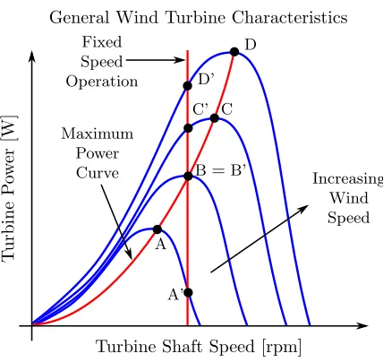
Wind turbines can be categorized into two main groups: fixed speed and variable speed. Although simple and robust, fixed speed turbines suffer from the unavoidable disadvantage that they cannot operate to efficiently capture the energy in the wind [6]. This is because they can only operate at one speed and wind speed is variable. Every turbine has aerodynamic characteristics similar to those shown in Figure 1.1. For each wind speed there is a certain turbine shaft speed that produces maximum power. A fixed speed turbine can only operate at maximum aerodynamic efficiency for one particular wind speed. As the wind varies from this speed the efficiency of the wind turbine is reduced. Therefore to capture the most amount of power from the wind, the turbine must be made to operate at variable speeds and to follow the curve of maximum power extraction.
General Wind Turbine Characteristics
T
urbine
P
ow
er
[W]
Turbine Shaft Speed [rpm]
Increasing Wind Speed Fixed
Speed Operation
Maximum Power Curve
A
A’
B=B’ C C’
D D’
Figure 1.1: General Turbine Characteristics: A variable speed turbine capable of tracking the max-imum power curve will extract more power than a fixed speed turbine for every wind speed except one, (B = B’) in the diagram.
and the speed of their shafts.
fgrid=nm·Pp
60 , (1.1)
wherefsis the output frequency in Hz,nmis the speed of the shaft in rpm, and Pp is the number
of pole pairs. Keeping the frequency a steady 50 or 60 Hz to match the power grid is a requirement for the wind turbine to connect to the grid. However, if the speed of the shaft is varying along with the wind speed, then so will the frequency. This means a power converter needs to be placed in between the turbine’s generator and the grid. Figure 1.2 shows this configuration. This converter needs to handle the entire power that the turbine produces. This type of configuration is necessary for wound rotor and permanent magnet synchronous generators.
Full-Scale Converter
Grid Transformer
PMSG or SG
50 or 60 Hz Variable
Frequency
Figure 1.2: Turbine Configuration Using Full-Scale Converters and Synchronous Generators
1.1.1
The Doubly-Fed Induction Generator Configuration
terminals by the use of slip rings. Direct access to the rotor windings increases the flexibility of the control of this generator. The major drawback of other types of generators is that their rotors have a fixed field, exerted by permanent magnets or direct currents. That means whatever speed their rotors are turned is the same speed that the rotor field will sweep over the stator windings and thus the frequency of the power available at the stator windings is directly related to that rotor speed. With the ability to directly inject variable frequency alternating current into the spinning rotor windings, the WRIM can ensure that the addition of the variable speed shaft and its field add to a constant 60 or 50 Hz. This will be explained in Section 2.1.2. The consequence is that the stator can be directly connected through a converter to the grid, as can be seen in Figure 1.3. The advantage of moving the converter from the stator to the rotor is that its size can be dramatically reduced, making it cheaper. The next section explains this in detail.
Grid Transformer
DFIG
50 or 60 Hz
Variable
Frequency 50 or 60 Hz
Partial-Scale Converter
Figure 1.3: DFIG Configuration Using Partial-Scale Converters
1.1.1.1 The Advantage of a DFIG Configuration
As stated, the main advantage of employing a DFIG is that the converter needed to control the machine is moved to the rotor, and the rotor can be made to handle significantly less power than the stator but still be able to control the power through the stator.
The power handled by the rotor is roughly proportional to the slip or relative speed difference from synchronous speed. This will be shown in Section 2.2.1. The relationship between the frequency and rotor speed of a WRIM is the same as that of any other machine, given in Equation 1.1, if its rotor is supplied with direct currents. As the rotor speed spins slower or faster than synchronous, the slip begins to increase. The power flowing stays proportional to this slip and everything keeps working if the proper frequency alternating currents are injected into the rotor. Now by limiting the speed range around synchronous, the power flow through the rotor is limited as well. If the speed range was extended all of the way to zero, or all of the way to twice synchronous, then the rotor would have to handle full power and the advantage would be lost. Fortunately, to cover the normal range of wind speeds that exist in nature, it has been found that the slip range only needs to extend about 30% above or below synchronous, so the power converter can be reduced to 30% as well [7].
can generate both below and above synchronous speed [7]. In Section 2.3.1 it will be explained how the DFIG can generate power from its stator for all speeds. Above synchronous speed additional power is generated by the rotor (supersynchronous generation) and below synchronous speed power is required to be injected into the rotor to sustain generation (subsynchronous generation). The fraction of power flowing through the rotor in either direction is related to the slip or speed difference from synchronous speed. This division of power through the rotor and stator is ideal for wind energy conversion.
More power is dealt with by the system as a whole for supersynchronous generation because the wind speed, generator speed and power in the wind are higher here. In fact, it will be demonstrated in Chapter 4 how the maximum power in the wind is proportional to the cube of the generator shaft speed. Therefore all stresses and limits imposed on the system’s power handling capabilities are set in this region.
The generator and turbine are sized together so that the rated power of the generator is not exceeded. Since a known proportion of the power will be carried by the rotor, the generator can be sized smaller than the maximum target turbine power by that same proportion. For example, see Figure 1.4, if a generator is rated at 2MW and the rotor converter is sized to handle 30% of that (600 kW), then the generator as a whole can be expected to produce 2.6 MW in total. The generator’s shaft speed is chosen through a gearbox ratio to achieve this target power at a speed that corresponds to 30% over synchronous. By setting this condition, the turbine and generator are now matched up well to gather maximum power for a large range of wind speeds. In the supersynchronous region, the power is split between the stator and rotor. At the rated wind speed the turbine is delivering its maximum target power, the stator provides most of it with its rated power and the rotor converter handles the rest, operating near its maximum capacity as well. Any speed in the supersynchronous region below this maximum speed results in a lower power level overall which does not overload either component.
0.5 1.0 1.2 1.3
0.5 0 −0.2−0.3
0.15 1.2
2.0 2.6 1.3
1.0
0.6
0.075
p.u. MW
Mec
hanical
P
ow
er
ωmech
ωsync slip
Subsynchronous Supersynchronous
vwind,rated
Suitability of the DFIG for Wind Energy Conversion
Rated Generator Power Rated Wind Turbine Power
|Pmech|
|Pmech|
|Ps|=|Pmech|+|Pr|
|Pr|
|Pgrid|=|Pmech|
|Pgrid|=|Pmech|
|Ps|=|Pmech| − |Pr|
|Pr|
Subsynchronous Supersynchronous
1.2
Control Strategies for DFIGs
A few main control methodologies have become popular for DFIGs in wind turbine applications. The most prevalent in literature are vector control, and direct torque or power control. Control of the torque constitutes control of any rotating machinery [8]. Direct torque control is a technique that aims to control the magnitude and angle of the rotor flux, to directly control torque. Since torque is the cross product of stator and rotor flux, and since the stator is connected to the grid, the stator flux is almost constant, and thus the rotor flux is the chosen control variable. This technique has been applied with success [9]. Its main drawback is the non-constant switching frequency it imposes on the converter [7].
1.2.1
Vector Control
Vector control was the first technique proposed for DFIGs in wind applications [10] and is still the most common in literature [7]. In this technique the rotor current is separated into two components, one responsible for the torque and the other for the magnetization of the machine. In this way the aim is to emulate the simple control structure of a DC machine [11]. To break the current into two components different reference frames can be used. The two most common are aligning to the stator flux [10] or the stator voltage [12]. Stator flux oriented vector control is the classical method and will be studied in Chapter 5.
Once the torque and flux are under control, the currents are related to the real and reactive powers of the machine. This is easier to do if the stator voltage reference frame has been used [7], but it has been achieved in the stator flux oriented frame by several researchers includingTapia et al. [13]. This decoupling or separate control of power is ideal for a wind turbine. The real power can be set to extract the maximum available power from the turbine and the power factor can be independently regulated [6].
1.3
Thesis Overview
In the textbook “Advanced Electric Drives: Analysis, Control and Modeling using Simulink®,” Mohan et al. establishes a working model of a vector controlled induction machine [8]. In that work, the gaps between theory and practical simulation are completely filled with clear explanations. The simulations are proven with provided scripts and models. This makes learning the subject manageable for new students in the area. The undertaking in this dissertation aims to extend this treatment to a DFIG wind turbine system. It is the intention of the author to quickly get the reader familiar with the mathematical constructs, the basic physics of the machines and the control theory necessary to construct a working model. Provided along with the theory is a working simulation model in the Simulink®environment with initializing scripts, on the accompanying CD-ROM.
Chapter 2
Steady State Analysis
There are two main purposes for studying the steady state operation of the system. The first is purely for a deeper understanding of the characteristics, modes of operations and power flow. The second is to solve for a steady state operating point and calculate the values of all variables needed to initialize the dynamic model. This initialization procedure will be covered in Section 2.5.
2.1
The Steady State Equivalent Circuit of a DFIG
The steady state equivalent circuit of an induction machine is a widely known topic cover thoroughly by many authors. Figure 2.1 shows the standard model for a caged machine [14, 15, 16]. The
Rs jωsLls jωsLlr Rr
Rr1−ss
jωsLm
Is Ir
Im
Vs
Figure 2.1: Caged Rotor Induction Machine Equivalent Circuit
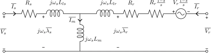
modification for a doubly fed operation is simply to include the rotor voltage Vr, see Figure 2.2,
Rs jωsLls jωsLlr Rr Rr1−ss
jωsLm
Is Ir
Im
Vs Vr
Vr1−ss
jωsλs jωsλr
Figure 2.2: Doubly Fed Induction Machine Equivalent Circuit
2.1.1
Elementary Two Pole Machine
Due to symmetry, the same interaction of variables occurs in each set of the machine’s poles. Cal-culations of the electrical variables for all sets of poles would be redundant, so they are done on just one pole pair. Mechanically the speed and torque of the machine depend on all the poles, so their quantities need to be adjusted.
Mathematically, this simplification is implemented by defining a new angle in “electrical radians” to replace the physical angle measured in “mechanical radians”;
θm=Ppθmech, (2.1)
where Pp is the number of pole pairs in the machine, θm is the position of the machine shaft in
electrical radians andθmechis the actual position of the machine shaft in mechanical radians. This
has the effect of stretching one pole pair over the circumference of the whole machine, see Figure 2.3. As a consequence, the electrical phase lag angle of sinusoids in the machine will correspond one to one with the position of the space vector representing them, see Section 3.3.1.3. It is important to note that for the remainder of the thesis every angular position and consequently every angular velocity has been defined in this fictitious two pole environment. When it is necessary to find the machine’s speed or torque, they need to be scaled by the appropriatePpconstant. Thus the mechanical speed
of the shaft is given by
60◦mechanical 180◦electrical
Quantity Mechanical Radians per Second Electrical Radians per Second
rotor angular velocity ωmech ωm
rotor angular frequency ωrotor ωr
stator angular frequency ωstator ωs
synchronous angular frequency ωsync ωg
Table 2.1: Angular Velocity and Frequency Notations
ωmech=
ωm
Pp
, (2.2)
where ωm is the angular velocity of the machine shaft in electrical radians per second andωmech
is the actual angular velocity of the machine shaft in mechanical radians per second. To be clear, Table 2.1 denotes the notations used for the angular velocities and frequencies that are expressed in both mechanical and electrical radians per second.
The torque derived in Section 2.4 and Section 3.4.4 must have the constant Pp as well because
it is derived from 2-pole variables. Each pole pair will contribute the same amount of torque so multiplying the torque for two poles by the number of pole pairs will give the total machine torque.
2.1.2
Slip and Frequency Relations
The frequency of the waveforms in the stator and rotor winding are related to the speed of the machine. In the most general sense the relationship is expressed by [17],
ωmech=ωstator±ωrotor (2.3)
where ωmech is the angular velocity of the shaft andωstator andωrotor are the angular frequencies
of the waveforms in the stator and rotor windings respectively. The negative sign applies when the phase sequence of the rotor is the same as the stator and the positive sign applies when the stator and rotor are in phase opposition.
With a wound rotor induction machine, both the stator and rotor are free to be injected directly with any frequency or phase sequence desired and the resulting shaft speed is given by Equation 2.3. In the doubly fed configuration for wind turbine applications, see Figure 1.3, the stator terminals are tied to the grid and the shaft is connected to the turbine. The rotor terminals are connected to an inverter capable of injecting any frequency or phase sequence.
Since the stator is tied directly to the grid, its frequency is constant and determined by the frequency of the grid. The stator excitation establishes the rotating magnetic field in the machine, and the speed at which it rotates is known as synchronous speed. Its speed depends also on the number of poles in the machine [14],
ωstator=ωsync=
2πfgrid
Pp
, (2.4)
whereωsyncis the synchronous speed in mechanical radians per second,fgridis the grid frequency
With the stator frequency and shaft speed determined, the rotor frequency that should be injected can be determined by rearranging Equation 2.3,
ωrotor=
ωmech−ωsync, phase equivalence
ωsync−ωmech, phase opposition
. (2.5)
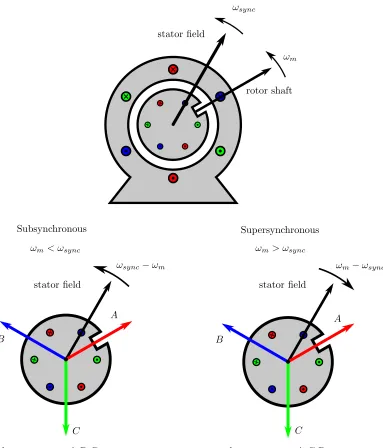
The need for the rotor frequency to switch phase sequence is illustrated in Figure 2.4. The stator
ωm
ωsync
stator field
rotor shaft
ωm< ωsync ωm> ωsync
ωsync−ωm ωm−ωsync
Subsynchronous Supersynchronous
A
stator field stator field
C B
A
C B
phase sequence: A-B-C phase sequence: A-C-B
Figure 2.4: Reversal of Rotor Phase Sequence as Rotor Crosses Synchronous Speed
field rotates counter-clockwise at ωsync. The rotor also rotates counter-clockwise at ωmech. The
machine is working in. The images at the bottom of Figure 2.4 are referenced to the rotor. That is the observer is placed on the rotor and thus the rotor is viewed as stationary. Now the observer will see the stator field rotating at a relative speed. In the first case the rotor is spinning slower than synchronous speed. The rotor would see the stator field, still travelling counter-clockwise but at the slower relative speedωsync−ωmech. The stator field would sweep over the rotor coils in the sequence
A-B-C and induce voltages of that sequence. For the second case, the rotor is spinning faster than the stator field. Now an observer on the rotor would see the stator field travelling clockwise at a speed ofωmech−ωsyncrelative to the stationary rotor, even though it is actually travelling
counter-clockwise relative to the stator. Thus the stator field would sweep over the rotor coils in the sequence A-C-B, and reverse the phase sequence of the induced voltages.
The relative speed difference from synchronous is so important to the operation of an induction machine that a new variable denoted as slip (s) is defined [14],
s= ωsync−ωmech
ωsync
. (2.6)
Notice that if the rotor speed is less than synchronous speed, the slip is positive and if the rotor speed exceeds synchronous speed the slip becomes negative. It is useful to express angular frequencies and velocities to each other using the slip for derivations later on,
ωrotor=sωsync, (2.7a)
ωr=sωs, (2.7b)
ωmech= (1−s)ωsync, (2.7c)
ωm= (1−s)ωs. (2.7d)
2.1.3
Equivalent Turns Ratio
Throughout this work, the rotor voltages and currents will be calculated with the parameters shown in Figure 2.2. However, the magnitudes will not be what actually exists in the machine. The rotor parametersRrandLlr are referred to the stator. This is standard practice for an induction machine;
the rotor’s parameters usually have to be measured on the stator side because there is no access to the rotor. The rotor parameters of a WRIM can be measured directly from the rotor’s terminals. However it is still beneficial to refer the rotor parameters to the stator to simplify the calculations. A definite turns ratio exists between the stator and rotor windings [7],
EM Fs
EM Fr
=skrNr ksNs
= s
T R, (2.8)
whereEM FsandEM Frare the induced electromotive forces (emfs) in the windings,NsandNrare
the number of turns of the windings,KsandKrare winding factors which depend on the geometry
of the machine and are slightly smaller than 1, s is the slip andT R is the equivalent turns ratio. Note that the quotient ks
s= 1 and the turns ratio of the windings is expressed as,
T R= KsNs
KrNr ≈
Ns
Nr
, (2.9)
The actual value of the rotor’s parameters are
Rr,act=
Rr
(T R)2, (2.10)
and
Llr,act=
Llr
(T R)2. (2.11)
Since all calculations are done with the referred values, the only purpose of these equations would be to refer the rotor parameters to the stator side if they were measured directly from the rotor’s terminals. The actual voltages and currents in the rotor are important. The machine’s rotor windings are rated for specific voltages and currents, so determining what the coils are actually subjected to is necessary. The actual voltage and current in the rotor can be calculated with
Vr ,act= Vr
T R, (2.12)
and
Ir ,act=Ir·T R. (2.13)
As a final note, all calculations done in this work use the rotor parameters referred to the stator, thus Equations 2.12 and 2.13 would be necessary for practical implementation.
2.1.4
Steady State Equations
The equations can be found by applying Kirchoff’s voltage and current laws to the equivalent circuit in Figure 2.2. The stator voltage is given by,
Vs=RsIs+jωsλs, (2.14)
whereλsis the stator flux linkage phasor. The rotor voltage is given by,
Vr=RrIr+jωrλr, (2.15)
whereλr is the rotor flux linkage phasor. The stator and rotor flux linkages are given by,
λs=Lm(Is+Ir) +LlsIs
whereLs=Lls+Lmand,
λr=Lm(Is+Ir) +LlrIr
=LmIs+LrIr, (2.17)
where Lr =Llr +Lm. These four equations fully describe the interaction of voltage, current and
flux linkage in the machine. Often it is useful to solve for the current explicitly,
Is=
λs Lm
λr Lr
Ls Lm
Lm Lr
= Lrλs−Lmλr
LsLr−Lm2
=λs
1
σLs−
λr
Lm
σLsLr
, (2.18)
Ir=
Ls λs
Lm λr
Ls Lm
Lm Lr
= Lsλr−Lmλs
LsLr−Lm2
=λr
1
σLr−
λs
Lm
σLsLr
, (2.19)
whereσ= 1− L2m
LsLr is the total leakage factor.
2.2
Power Balance Relations
The equivalent circuit in Figure 2.2 completely neglects any mechanical power losses and the electrical core losses. This model has been chosen to match up with the complexity of the dynamic model required for control [7], so that it can be used in Section 2.5 for initialization of the model through a steady state solution. It is still more than detailed enough to describe the basic power balance and flow through the machine. The purpose of this section is to give an idea how power flows in the four different modes introduced in Section 2.3.
2.2.1
Active Power Balance
This discussion will concentrate on the active power in the machine. Figure 2.5 shows where each power is accounted for in the equivalent circuit and shows the direction which corresponds to the power flow that results when the respective power is positive.
First of all there are three places active power can be injected or removed from the machine; the stator terminals, the rotor terminals and the rotor shaft. Additionally some active power is dissipated as heat from the stator and rotor winding resistances. Notice the assumed current directions in Figure 2.5, both stator and rotor currents are assumed to be entering the machine, that is they are in motoring convention. This means that a positivePs orPrimplies the machine is consuming power
from the respective terminals and negativePs andPr implies the machine is supplying power from
the respective terminals,
Rs jωsLls jωsLlr Rr Rr1−ss
jωsLm
Is Ir
Im
Vs Vr
Vr1−ss
Ps Pr
Pcu,s Pcu,r Pmech,Rr Pmech,Vr
Pmech
Figure 2.5: Active Power Associated with Each Equivalent Circuit Parameter
Pr= 3Re{VrIr∗}. (2.21)
In the motoring convention,Pmechis chosen positive for motoring power; that isPmech>0 implies
that the machine is producing mechanical torque. Pmech < 0 implies that the machine requires
mechanical power from an outside source, the prime mover. In the equivalent circuit Pmech is
represented by the two terms with slip in them;Rr 1−ssandVr 1−ss. Care must be taken when
writing the expression for mechanical power modelled by this source. The mechanical power modelled by the resistorRr 1−ssis
Pmech,Rr = 3|Ir| 2R
r
1
−s s
. (2.22)
WhenPmech,Rr is positive it represents dissipation of electrical power, which matches the definition of Pmech where electrical power is converted to mechanical for positive values. Note that a
nega-tive value of slip will make Pmech,Rr negative, which means it is supplying electrical power. The mechanical power modelled by the voltage sourceVr 1−ssis
Pmech,Vr = 3
1
−s s
Re{VrIr∗}. (2.23)
Notice the voltage is in source convention; the current is leaving the positive terminal. This is in opposition to the definition of Pmech since a positive value of Pmech,Vr means electrical power is injected into the circuit. The reason for choosing this polarity forVr 1−ss was to match with the
polarity of Vr when separating Vsr into Vr and Vr 1−ss. Now the full expression for mechanical
power can be written,
Pmech=Pmech,Rr−Pmech,Vr = 3|Ir|2Rr
1
−s s
−3
1
−s s
Finally, the power dissipation from the stator and rotor winding resistances are given as,
Pcu,s= 3|Is|2Rs, (2.25)
and
Pcu,r= 3|Ir|2Rr. (2.26)
respectively.
The power in the stator and rotor pass to each other through the air gap. For motoring convention, positive power at the air gap implies power flowing from the stator to the rotor. On the stator side,
Pag =Ps−Pcu,s, (2.27)
on the rotor side,
−Pag =Pr−Pcu,r−Pmech, (2.28)
therefore the power balance of the entire machine is,
Ps+Pr=Pcu,r+Pcu,s+Pmech. (2.29)
All power on the stator side is electrical in nature while the rotor is host to both mechanical and electrical power. Electrical power in the rotor is sometimes referred to as slip power [18],
Pslip=Pcu,r−Pr
= 3|Ir|2Rr−3Re{VrIr∗}. (2.30)
because its magnitude is proportional to slip. The balance of mechanical power in the rotor can be seen by comparing Equations 2.30 and 2.24 to the total power passing through the rotor, (see Figure 2.1),
−Pag = 3|Ir|2
Rr
s −3Re{VrIr
∗
}1s. (2.31)
Now it is apparent to see,
Pslip=sPag, (2.32)
and,
Pmech= (1−s)Pag. (2.33)
2.2.2
Reactive Power Balance
Rs jωsLls jωsLlr Rr Rr1−ss
jωsLm
Is Ir
Im
Vs Vr
Vr1−ss
Qs Qr
QLls QLlr
Qvir
QLm
Figure 2.6: Reactive Power Associated with Each Equivalent Circuit Parameter
equivalent circuit it is seen where reactive power flows in the machine. Figure 2.6 shows which elements consume reactive power and where it is injected in the model. The leakage and magnetizing inductancesLls,Llr andLmconsume reactive power denoted byQLls, QLlr andQLm respectively. The stator and rotor terminals are ports that can exchange (either consume or supply) the reactive power Qs and Qr. Additionally there is a voltage sourceVr1−ss which can exchange the reactive
powerQvir. By analysing the model in a completely mathematical sense, the reactive power balance
is seen as,
QLls+QLlr+QLm =Qs+Qr+Qvir, (2.34) where,
Qs= 3Im{VsIs∗}, (2.35)
Qr= 3Im{VrIr∗}, (2.36)
QLls= 3|Is| 2ω
sLls, (2.37)
QLlr= 3|Ir| 2ω
sLlr, (2.38)
QLm= 3|Is+Ir| 2ω
sLm, (2.39)
Qvir= 3Im{1−ssVrIr∗}. (2.40)
Note that QLls, QLlr, QLm, Qs and Qr have physical meaning, where as Qvir is more obscure. According to [19] the termQvir which arises from the voltage source 1−ssVris a virtual effect of the
external circuit and is necessary to include when the circuit manipulations to reduce the rotor to the stator are applied. The reactive power introduced to the circuit from this modelling element actually comes from the external circuit (the power converter).
2.3
Modes of Operation
operation depicted on the left of Figure 2.7, provided they are connected to a capable drive. That is they can motor and generate in the forward and reverse directions. The ability to reverse direction
0 Tem
ωm
subsynchronous motoring
ωm
Tem
ωm Tem ωm
Tem
ωm Tem
ωsync
0 Tem
ωm
motoring forward generating forward
motoring reverse generating reverse
ωm
Tem
ωm
Tem
ωm
Tem
ωm
Tem
subsynchronous generation supersynchronous
motoring supersynchronous
generation
Figure 2.7: Left: Standard Definition of Four Quadrant Operation, Right: Four Quadrant Operation in One Direction
is unnecessary in wind turbine applications; the turbine blades will always spin the shaft in the same direction. There is however still a relevant four quadrant operating region that can be defined for uni-directional rotation, see the right of Figure 2.7. Induction machines are designed to operate around their synchronous speed. When the shaft spins slower than synchronous speed it is known as subsynchronous operation and the machine can only motor. When the shaft spins faster than synchronous speed it is known as supersynchronous operation and the machine can only generate. This is because the direction of the induced torque in an induction machine depends on the speed. A wound rotor machine can be made to generate or motor above or below synchronous speed and thus achieves this sort of four quadrant operation.
2.3.1
Power Flow
The exchange of power through the terminals of a wound rotor machine can be explained by ex-amining Equations 2.32 and 2.33. It will be seen that the intrisic nature of the flow is well suited for variable speed generation. For this discussion, the dissipated power in the stator and rotor resistances will be neglected to simplify the explanation and make the fundamental points clear.
2.3.1.1 Subsynchronous Motoring
This mode is characterized by Pmech>0, that is mechanical power is available at the shaft, and a
slip in the range of 0< s <1. From Equation 2.33,
Pag=
Pmech
1−s ⇒Pag >0 and|Pag|>|Pmech|.
From Equation 2.32,
Therefore power flows across the air gap from stator to rotor side. There is more power at the air gap than available at the shaft, and the extra power is present at the rotor terminals.
Ps
Pslip
Pag
Pmech
Figure 2.8: Power Flow in the Subsynchronous Motoring Mode
2.3.1.2 Supersynchronous Motoring
This mode is characterized byPmech >0 and a slip in the range of −1 < s < 0. From Equation
2.33,
Pag=
Pmech
1−s ⇒Pag >0 and|Pag|<|Pmech|.
From Equation 2.32,
Pslip=sPag ⇒Pslip<0.
As with subsynchronous motoring,Pag is still positive, it flows across the air gap from the stator to
the rotor. This time it is less thanPmechand the power required to sustain motoring must be input
to the rotor; this is seen byPslipbecoming negative.
Ps
Pslip
Pag
Pmech
Figure 2.9: Power Flow in the Supersynchronous Motoring Mode
2.3.1.3 Supersynchronous Generating
This mode is characterized byPmech<0, that is mechanical power needs to be input to the shaft,
and a slip in the range of−1< s <0. From Equation 2.33,
Pag=
Pmech
1−s ⇒Pag <0 and|Pag|<|Pmech|.
From Equation 2.32,
The main input to the system is in the rotor now, reversing the direction of Pag to transfer power
to the stator. The input mechanical power is greater than the air gap power and the extra power is available from the rotor terminals.
Ps
Pslip
Pag
Pmech
Figure 2.10: Power Flow in the Supersynchronous Generating Mode
2.3.1.4 Subsynchronous Generating
This mode is characterized byPmech<0 and a slip in the range of 0< s <1. From Equation 2.33,
Pag=
Pmech
1−s ⇒Pag <0 and|Pag|>|Pmech|.
From Equation 2.32,
Pslip=sPag ⇒Pslip<0.
As with supersynchronous generationPag <0 and power is transferred from the rotor to the stator.
This time the mechanical power is less than the air gap power and extra power must be injected into the rotor to sustain the generating mode. Electrical power in the rotor is sometimes referred to as slip power.
Ps
Pslip
Pag
Pmech
Figure 2.11: Power Flow in the Subsynchronous Generating Mode
2.4
Steady State Torque
of power and speed,
Tem=
Pmech
ωmech
. (2.41)
The simplest way to derive the torque in terms of electrical quantities is described in [7]. The mechanical power is written in terms of currents only employing Equations 2.24, 2.17 and 2.15. The result is derived in Appendix A.1,
Tem= 3PpLmIm{IsIr∗}. (2.42)
It is also possible to express the torque in terms of flux linkage. This way the expression can be directly compared to the dynamic torque equation, Equation 3.36 in Section 3.4.4. Using Equations 2.18 and 2.19,
Tem= 3Pp
Lm
LsLrσ
Im{λsλr∗}. (2.43)
The derivation is also given in Appendix A.1.
2.5
Steady State Solution
The complete steady state solution of the DFIG is obtained from solving Equations 2.14 through 2.19 and then solving for the power or torque desired. Since the actual machine is excited by applying voltages at the stator and rotor terminals, it seems logical to start with Vs and Vr as
known input values and then calculate the current and flux linkage. This solution path is not useful for the purpose of initializing the dynamic model because the rotor voltage will be determined by a controller and depends on other known values. In the dynamic model, the stator voltage is known and the rotor voltage will be controlled to achieve a target stator real and reactive power set point.
To start the solution, all parameters of the machine must be known. Since this is a steady state solution, a speed must be chosen as well. After the model for the wind turbine has been specified, the speed of the generator and its developed power will be derived from its characteristics. For this analysis, this amounts to s and Ps being known values. Additionally the desired reactive power
Qswhich can be chosen to make the machine conform to any power factor must be specified. The
stator voltage is also known, because it is fixed to the grid voltage, it will be taken as reference in the calculations.
Step 1: The stator phase voltage is specified from the rms line-to-line voltage of the grid,VLL,rms
and set as the reference:
Vs= VLL,rms√3 0◦. (2.44)
Step 2: The stator current is calculated from the reference power requirements, the total complex power exchanged at the stator is
Pref
s +jQrefs = 3VsIs∗. (2.45)
Rearranging, the current is found,
Is=
Pref
s −jQrefs
Vs∗
Step 3: Using Equation 2.16, the stator flux linkage is found:
λs=
Vs−RsIs
jωs
(2.47)
Step 4: Using Equation 2.19, the rotor current is found:
Ir=
λs−LsIs
Lm
(2.48)
Step 5: Using Equation 2.17, the rotor flux linkage is found:
λr=LmIs+LrIr (2.49)
Step 6: Using Equation 2.15, the rotor voltage is found:
Vr=jωrλr+RrIr (2.50)
Once these six variables are known, calculating any power or torque is trivial. Finding the steady state rotor voltage to achieve a particularPref
s andQrefs also sets the stage for the machine
Chapter 3
Dynamic Model of a Wound Rotor
Induction Machine
3.1
Brief Introduction to the Model
The dynamic model chosen for this work is a standard used for induction machines by many authours in the field of machine analysis [8, 11, 20]. Like all dynamic models it consists of coupled differential equations. The model is of fifth order; four equations describe the interaction of electrical variables and one is used to characterize the mechanical subsystem. Electromagnetic torque is the single most important variable as it is the link between electrical and mechanical subsystems. The number of equations used to define each aspect shows that this model favours the electrical side and treats the mechanical side as fundamentally as possible.
3.2
Simplifing Assumptions
The end purpose of this model is to be used for the control of the machine. As such it is idealized to contain only the most important interaction of variables and ignores complicating features.
The machine is treated as though it is symmetrical down its entire axis, no end effects are taken into account. This allows for all information about the machine to be contained in two dimensions, in a cross section of the machine. The air gap is considered smooth with no slotting effects. The windings are idealized as being perfectly sinusoidally distributed. The flux in the air gap is directly entirely radially. The permeability of iron is infinite and their are no iron losses. There are no mechanical losses, friction or any forms of saturation taken into account.
3.3
Mathematical Concepts
This model relies on the use of space vectors and reference frames to define the variables in the equations. Many authors treat these concepts slightly differently. This section will serve to introduce these concepts, describing what they physically represent in the machine, and how they are used in the model. Furthermore it will clearly denote all notations and conventions for the rest of the thesis.
3.3.1
The Space Vector
The dynamic analysis and control of any electric machine is greatly aided by the mathematical construct known as a space vector. Mathematically a space vector is identical to any arbitrary vector, having a length and angle. It will be shown that they can be used to simultaneously represent the flux linkage, current or voltage in three phases allowing for compact equations. Furthermore they prove useful for easily writing the equations for the control of the machine and actually form the basis for the technique of vector control applied in this thesis.
3.3.1.1 Physical Interpretation of a Space Vector
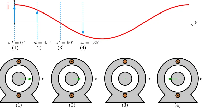
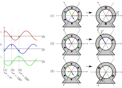
The flux density in the air gap from an ideally sinusoidally distributed, two pole coil is shown in Figure 3.1. It is sinusoidally distributed and directed radially [8]. The region of maximum flux density defines the direction for the axis of the coil; the positive direction is chosen for flux pointing from the rotor to the stator. A space vector is used to represent this complex distribution. The direction of the vector is pointed along the axis of the winding; the space where the flux density is highest. The length or magnitude of the vector is proportional to the flux density of the field at a particular time. That is, a space vector is an instantaneous quantity, capable of representing variables at each instant of time, as they change. Note that the fact that the field is sinusoidally distributed around its peak is unimportant for the dynamic model leading to the control of the machine, and does not need to be represented by the space vector; only the magnitude of the field density and its position are of concern. Also note that the distributed coil is treated as a single concentrated winding.
Since the stator is unmoving and the windings are mounted inside it, the axis for any coil is also
reference axis
locked in position. As a sinusoidal excitation is applied to the winding, the peak flux density remains in the same direction, but the magnitude varies sinusoidally, see Figure 3.2.
ωt
i
ωt= 0◦ ωt= 45◦ ωt= 90◦ ωt= 135◦
(1) (2) (3) (4)
(1) (2) (3) (4)
Figure 3.2: Space Vector Representing Instantaneous Field Density from One Winding
The machine under study in this work is a three phase wound rotor induction machine. It contains three windings on the stator and rotor. The machine is constructed such that the axis of the coils will be separated 120◦ electrically from each other, see Figure 3.3.
a-axis b-axis
c-axis
−→
Fa
−→
Fb
−→
Fc
120◦
240◦
Figure 3.3: Three Phase Axis Placement in Electrical Degrees
−→
Fs
(2)
−→
Fs
(1)
−→
Fs
(3)
ωt
ωt
ωt
ωt=
0◦
ωt=
120 ◦
ωt=
240 ◦ (1) (2) (3)
ia
ib
ic
Figure 3.4: Three Phase Rotating Space Vector
electrical phase lag in the excitation waveforms.
Although only the magnetic fields physically exist in space, the space vector concept can extend to describe current and voltage. Note in Figure 3.4 that the three windings can be replaced with just one fictitious winding that is larger and oriented to the resultant field. Now a fictitious current and voltage in and across this coil, that would be responsible for this resultant field can be defined. For modelling purposes these space vectors are a tool which allow the machine equations to be written compactly, with contributions from all three phases in just one variable. The instantaneous value of any variable can quickly be found by projecting the space vector back onto each respective axis and multiplying it by a constant as defined in the following sections.
3.3.1.2 Definition of Space Vector Notation
in Figure 3.5.
−
→
v
s
r
reference frame: s, r, g
machine member: s, r
variable: λ, v, i
Figure 3.5: Space Vector Notation
3.3.1.3 Mathematical Description of a Space Vector
A space vector, having a magnitude and phase is expressed as a complex number, and is similar to the well known time phasor. The first major difference is that the magnitude varies with time, so it is a function of time. Secondly, the phase represents a physical angular displacement and must be referenced to some axis in space. For the stator, the positive a-axis is taken as the reference, see Figure 3.3. Therefore, the space vector components along each phase axis are1
− →
va s
=va(t) 0◦ =va(t)ej0, (3.1a)
− →vbs
=vb(t) 120◦=vb(t)ej
2π
3 , (3.1b)
− →vcs
=vc(t) 240◦=vc(t)ej
4π
3 . (3.1c)
The space vector is found by adding the contributions from each phase
− →vss
=−→va s
+−→vb s
+−→vc s
=va(t)ej0+vb(t)ej
2π
3 +v
c(t)ej
4π 3
=vs(t)ejθvs. (3.2)
Nowva(t),vb(t),vc(t) are a balanced set;
va(t) =Vcos(ωt+φ), (3.3a)
vb(t) =Vcos(ωt+φ−23π), (3.3b)
vc(t) =Vcos(ωt+φ−43π). (3.3c)
Substituting Equation 3.3 into 3.22,
1stator voltage is taken for example
− →vss
=V cos(ωt+φ)ej0+V cos(ωt+φ−2π
3)e
j2π
3 +Vcos(ωt+φ−4π 3 )e
j4π 3
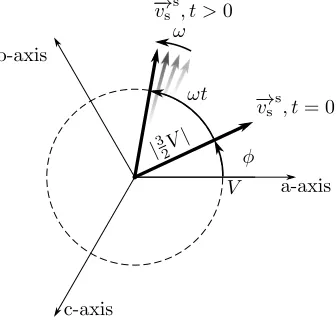
=32V ej(ωt+φ). (3.4)
First it is important to note that the magnitude of the space vector is 3
2 that of the peak of the input sinusoids. Second, the position of the space vector depends on time, and thus is rotating counter-clockwise at an angular speedω. Figure 3.6 shows the space vector at an arbitrary timet. Note that any phase shift in the input sinusoids shows up as the initial position of the space vector at timet= 0, this property will be exploited in Section 3.3.3 to find the correspondence between a space vector and the time phasor.
a-axis b-axis
c-axis
− →vss
, t= 0
φ
− →vss
, t >0
V
|32V|
ωt ω
Figure 3.6: Graphic Representation of Space Vector in Equation 3.4
3.3.2
Reference Frames and the Two-Axis Transformation
3.3.2.1 Clarke Transformation
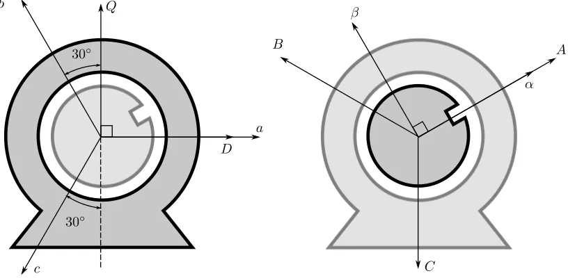
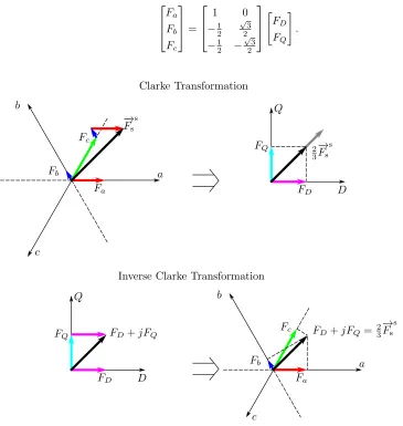
The Clarke transformation is probably the simplest form of two-axis transformation available. It maps the contributions from three axes directly to two. Figure 3.7 shows the axis placement for the Clarke transformation for stator and rotor quantities. For the stator, theD-axis is directly in line with the a-axis; theQ-axis leads it by 90◦. The matrix which maps the components is
"
FD
FQ
#
=c
"
1 −1
2 −
1 2 0 √23 −√3
2
#
Fa
Fb
Fc
, (3.5)
where F is just a general variable which could represent voltage, current or flux linkage. The entries in the matrix are easy to understand. TheD-axis is directly in line with the a-axis so its contribution is 1. The b and c axes are both 30◦ off the perpendicular to theD axis, in the opposite direction so they both contribute−sin(30◦) =−1
2. TheQ-axis is completely orthogonal to the a-axis so there is 0 contribution. The b and c axes are 30◦ off the positive and negative Q-axis respectively, so their contributions are cos(30◦) =√3
2 and−cos(30◦) =−
√
3
2 respectively.
a D b
c
Q
30◦
30◦
α β
B A
C
Figure 3.7: Stator and Rotor Reference Frames Overlaid on their Respective Three Phase Axes
There is a constant of proportionality cin Equation 3.5 which has not been defined yet. By trans-forming 3 axes to 2, the variables in their equations no longer represent real magnitudes. In fact the transformation creates a fictitious calculation environment which is separate from the real world; as long as the relative magnitudes of the components remain proper, when they are converted back with the inverse transform, everything will work out. This leaves a degree of freedom when performing the transformation, it can be scaled by any number and it will work when transformed back. There are however advantages to choosing certain values and the most prevalent are c= 2
3 andc =
q
2 3. The first choice allows the peak values of the variables in the two axis frame to equal those in the three axis frame. Recall Equation 3.4 where the space vector for a balanced three phase set was derived. Its magnitude was 3